Short-term market reaction after extreme price changes of liquid stocks

Abstract

In our empirical study, we examine the price of liquid stocks after experiencing a large intraday price change using data from the NYSE and the NASDAQ. We find significant reversal for both intraday price decreases and increases. The results are stable against varying parameters. While on the NYSE the large widening of the bid-ask spread eliminates most of the profits that can be achieved by a contrarian strategy, on the NASDAQ the bid-ask spread stays almost constant yielding significant short-term abnormal profits. Furthermore, volatility, volume, and in case of the NYSE the bid-ask spread, which increase sharply at the event, decay according to a power-law and stay significantly high over days afterwards.

This paper focuses on intraday market reaction to stock price shocks. It is only recently that such minute-to-minute analysis of stock prices has been made possible by the fast improvement of computers.¹ Detailed studies have been devoted to intraday reaction on interest rates and foreign exchange markets following macroeconomic announcements (e.g. that of ?). A thorough empirical study of the intraday reaction to price shocks on stock markets is still missing.

Many studies in the past have been devoted to investigating the abnormal returns following large price changes. In the vast majority of cases research is focused on daily price decreases of at least 10%. Significant price reversal is found during the first 3 post-event days on all stock markets investigated: overreaction is found on the NYSE (New York Stock Exchange) and the AMEX (American Stock Exchange) by ?.² On the other hand, in case of large price increases either no overreaction is found (? on the TSE) or the size of the price reversal is much less robust than those following price decreases (? on the NYSE).

In contrast to long-term overreaction (with a time span of years), such as that found by ?, which may be at least partially attributed to a mismeasurement of the risk as described by ?, short term pricing errors are much more robust. In case such short-term overreaction yields abnormal profits it poses a major threat to the hypothesis of market efficiency. It is thus crucial to investigate the transaction costs a trader implementing a contrarian trading strategy faces. The most important source of transaction costs is the bid-ask spread: both ?, and ? compare the size of overreaction with that of the bid-ask spread after large daily price changes, and conclude that no significant profits can be achieved by arbitrageurs since the anticipated profit of a contrarian trading strategy does not significantly exceed the transaction costs: i.e. the reversal for daily data is significant statistically but not economically.

Thus, the pure existence of an overreaction does not pose a threat to market efficiency, although a full explanation of the phenomenon is still to be found. In spite of the fact that no abnormal profits can be made by external traders (those not owning stocks suffering serious one day losses) it still remains a puzzle why investors sell after large price decreases when a significant rebound is to be expected in the following days.

? show that on the NYSE the size of the overreaction after large daily price drops had diminished to zero until 1991. While in 1963–67 a significant rebound of 1.87% was to be expected on the first three days following the event day, the reversal sank to 0.06% in 1987–1991, which is not significant any more. This finding may as well imply that overreaction is a sign of market inefficiency which was corrected by market participants after being revealed.

The studies mentioned above all deal with daily close-to-close price changes. These price changes are due at least partially to news received by the traders during this 24 hour period, although ? show, that in many cases it is hard to trace back large changes in the S&P 500 index to one particular event. Such a time interval may be too long, since many events can take place during one day. Some events may take place within a day and thus cannot be unveiled studying daily data. Recent research of intraday data by ? shows that new information is incorporated in stock prices within 5–15 minutes. This is in full correspondence with the fact that autocorrelation of stock prices diminishes to zero in about the same time (?). Hence we might as well expect that it is worthwhile to examine big intraday price changes of the length from a couple of minutes to a couple of hours. For example ? introduces a method in order to find large intraday changes in the S&P 500 index which occur within 5 minutes. Instead of an index we concentrate on large price changes in the price of individual stocks, and follow a similar, but somewhat more thorough approach when searching for intraday price shocks, focusing on large price changes and potential reversal within the trading day. Searching for the cause of the extreme price changes, although interesting, is not the task of our study and is not relevant from the point of testing weak-form market efficiency.

Intraday price changes are interesting not only because of the possibility of arbitrage but for pure academic reasons too: the whole price discovery process takes place within the active trading period. The understanding of this process is not possible without following the exact intraday transaction bid and ask price evolution. ? point out the importance of such minute-to-minute empirical investigation which could not yet be carried out when their paper was written in 1986: now we have the data and computers have the capability of doing such intraday analysis.

Recently much research has been devoted to the price discovery process using high resolution data.³ The dynamics of the whole limit order book has been investigated thoroughly during the past years.⁴ Here we focus on extremal events in the hope that the dynamics after them will contribute to revealing the complex mechanism of price formation.

In case of examining intraday price changes we use minute price data, thus we only examine liquid stocks: those which are traded minute-to-minute during the trading day. This restriction is useful in the sense as well that liquid stocks are less exposed to bid-ask effects (infrequent trading), and thus the transaction price gives us more direct information on the price traders assume to be appropriate for the given stock. Additional information on the minute-to-minute trading around the event can be obtained by studying the minute volatility and the trading volume which are also subjects to our studies. We consider two different markets in order to point out possible differences due to the various trading mechanisms. Indeed, as we show later, there are significant differences in the behavior of the NYSE and the NASDAQ.

The paper is organized as follows. We describe the dataset and the methodology of finding events in Section 1. Our empirical findings are presented and discussed in Section 2. Section 3 contains our conclusions.

1 Data and Methodology

The primary dataset used is the TAQ (Trades and Quotes) database of the NYSE for the years 2000-2002. The TAQ database is that supplied by the NYSE: it includes all transactions and the best bid and ask price for all stocks traded on the NYSE. In our sample, we include all stocks which were traded anytime during the observed period. After adjusting for dividend payments and stock splits, a minute-to-minute dataset is generated using the last transaction, and the last bid and ask price during every minute. If no transaction takes place for a minute (which is rare for liquid stocks on the NYSE), the last transaction price is regarded as the price. Determining the beginning and the end of the trading day is done using the dataset: the first trading minute for a given stock on a given day is the minute during which it was first traded that day, the last minute is the last minute for which the DJIA was calculated but not later than 16:00. ⁵ We define liquid stocks as those for which at least one transaction was filed for at least 90% of the trading minutes of the stocks included in the DJIA during the 60 pre-event trading days.

The secondary dataset is the TAQ database of the NASDAQ. We include all NASDAQ stocks traded on the first trading day of 2000. Unfortunately no dividend and stock splits information is available in the TAQ database for the NASDAQ stocks. However, intraday analysis is not affected by stock splits. In case of the NASDAQ determining the opening minute is straightforward, since the trading is computer based.⁶ A problem arises when using NASDAQ data: there are often singular transactions filed at a price outside the bid-ask spread (sometimes even 4-8% from the mean bid-ask price). Since these do not represent a change in investor sentiment they are to be excluded from the sample. Thus the specified trigger levels have to be surpassed by not only the intraday transaction price change alone but by the change in the mean of the bid and ask price as well.

We do not include events in our sample for such stocks where the price tick is high compared to nominal price either: thus only stocks with a nominal price over 10 USD are studied. Since we study the intraday reaction to large price shocks we first have to define what ”extreme price changes” mean. Here we restrict ourselves to pure intraday price changes: large changes at the beginning of the day (close-to-open) do not seem to show any extraordinary effects which are stable to varying the trigger parameters.

1.1 Defining large intraday 15-minute price changes

We use a combined trigger to find the intraday events. Two trivial methods are at hand:

1. Absolute filter: using this first method we look for intraday price changes bigger than a certain level of 2-6% price change within 10-120 minutes. In this case we have to face several problems. Most of the events we find occur during the first or last couple of minutes of the trading day because of the U-shape intraday volatility distribution of prices (see ?). These events represent the intraday trading pattern rather than extreme events. Another problem is that a 4% price jump e.g. may be an everyday event for a volatile stock while an even smaller price move may indicate a major event in case of a low volatility stock.

2. Relative filter: in case of this second method we measure the average intraday volatility as a function of trading time during the day: this means measuring the U-shape intraday 10-120-minute volatility curve (length chosen corresponding to the length of the price drop we are going to study) for each stock prior to the event. ⁷ We define an event as a price move exceeding 6-10 times the normal volatility during that time of the day. The problem in case of this method is the following: since price moves are very small during the noon hours, the average volatility for the 60 pre-event days in these hours may be close to zero, i.e. a small price movement (a mere shift from the bid price to the ask price for example) may be denoted as an event. In this case the events cluster around the noon hours and no events are found around the beginning and the end of the trading day.

The best solution for localizing events is a combined one. Using the relative filter and absolute filter together, we can eliminate the negative effect of both filters and combine their advantages. Thus an event is taken into account if, and only if, it passes both the relative and the absolute filter. We adjust the absolute and relative filter so as to achieve that events are found approximately evenly distributed within the trading day. In addition we omit the first 5 minutes of trading because we do not want opening effects in our average. We omit the last 60 minutes of trading as well because, as shown in Subsection 2.2.1, the major reaction after the price shock takes place during the 30-60 minutes after the end of the price change, and we would like to focus on the intraday price reaction before the market closes.

In order to be able to observe the exact price evolution after the intraday event, it is crucial to localize the events as precisely as possible. Since some price changes may be faster than others we allow shorter price changes than the given 10-120 minutes as well. For example if when looking for 60 minute events, the price change already surpasses the filter level in e.g. 38 minutes then we assume the price change has taken place in 38 minutes. The end of the time-window in which the event takes place is regarded as the end of the price change, and this is the point to which the beginning of the post-event time scale is set: thus minute 0 is exactly the end of the earliest (and the shortest of those) time window for which the price change passes the filter. This method is constructed so as to ensure that one can definitely decide by minute 0 whether an event has taken place in the preceding 10-120 minutes (time length depending on the specification of the filter) or not.

1.2 Calculating the average

Choosing the sample of events included in the average is again a crucial step. For convenience we only include the first event during a given day for a given stock in the average. A major event may affect the whole market, thus many stocks may experience a price shock at the same time. Including all events in the average would yield a sample biased to such major events. In order to avoid this bias no events are taken into account which happen within $T=60$ minutes of the previous event included in the average. The importance of not letting the post-event time periods overlap is discussed in detail in Appendix A.

When studying intraday price changes, 1 minute volatility, 1 minute trading volume, and the bid-ask spread are averaged besides the cumulative abnormal return, and the bid and ask price. Volatility, trading volume, and the bid-ask spread are measured in comparison to the average minute-volatility and minute trading volume of the individual stock during the same period of the trading day (intraday volume and volatility distributions are calculated using the average of the 60 pre-event trading days). This step is important in order to remove the intraday U-shape pattern of the above quantities from the average, since their intraday variation is in the same order of magnitude as the effect itself we are looking for.

When studying the intraday effect (within half an hour to one hour) during the trading day, the specific way of calculating abnormal returns seems unimportant since normal profits up to one hour can probably be neglected. It may however be the case that market returns are significantly different from the average during the post-event hours, thus the CAPM is used to calculate abnormal returns, where the DJIA index is used as the market portfolio for the NYSE and the NASDAQ Composite Index for the NASDAQ.⁸ The $\beta$ values for the individual stocks are calculated using daily (close-to-close) stock prices and index changes of the 60 pre-event trading days, since minute price changes are so noisy that no reliable $\beta$ values can be calculated from them. Since $\beta$ values may change after large price shocks, the post-event abnormal return is calculated using the $\beta$ computed using the 60 post-event trading days (if there are not enough post-event days in the data, the pre-event value is used).

Our results can be regarded as significant in case both abnormal and the unadjusted post-event returns are significant as well. We can conclude from the results in Section 2 that raw and abnormal (risk-adjusted) returns are not significantly different, which is not surprising in the light of the fact described above that expected returns for such short intervals as 30-60 minutes is practically zero. Thus we will stay with raw returns when analyzing the stability of our filter.

T-values are calculated as deviation of mean from null-hypothesis (0% in case of returns) over the standard deviation of the mean in each and every case.

2 Empirical results

2.1 Intraday price reaction

We present abnormal and raw returns after intraday 60 minute price shocks in Table 1 for the NYSE and Table 2 for the NASDAQ . The price changes included in the average are in absolute value all bigger than 4% and 8 times the average 60-minute volatility of the corresponding 60 minutes during the 60 pre-event trading days. These trigger values were determined using the NYSE dataset in order to find only extreme events, and to result in an approximately even distribution of events during the trading day: Table 3 shows the intraday distribution of events. Events are at least 60 minutes apart, thus only returns during a time period of maximum 60 minutes should be calculated in correspondence with Appendix A. Figure 1 shows the exact evolution of transaction, bid, and ask price around the event for NYSE and NASDAQ stocks: there is a clear reversal in case of both decreases and increases. The phenomenon of the bid-ask bounce, which ? claim is a substantial cause of daily price reversals on the NYSE, cannot be observed for intraday price reversal of liquid NYSE stocks, neither for NASDAQ stocks.

Figure 1: Price reversal after intraday price increases and decreases exceeding 4% and 8 times the pre-event volatility on the NYSE and the NASDAQ

Events are maximum 60-minute long price drops exceeding 4% and 8 times the average 60-minute volatility of the same time interval of the 60 pre-event days. Returns are raw returns. An average of 175 increases and 222 decreases on the NYSE and 273 increases and 215 decreases on the NASDAQ respectively. Minute 0 corresponds to the time when the price change exceeds the combined filter level.

Table 1: Price evolution after intraday price decreases and increases exceeding 4 % and 8 times the pre-event volatility for liquid stocks on the NYSE

Events are maximum 60-minute long price drops exceeding 4% and 8 times the average 60-minute volatility of the same time interval of the 60 pre-event days. Abnormal returns (AR) are calculated by subtracting beta times the corresponding index return (DJIA) from the raw return (RR) of the stock’s price on the basis of TAQ database. Pre- and post-event betas are calculated from 60 daily returns before and after the event. An average of 175 increases and 222 decreases at least 60 minutes from each other and at least 60 minutes before market closure. Minute 0 corresponds to the time when the price change exceeds the filter level. T-values in parenthesis.
from to increase decrease time (minutes) AR RR AR RR -120 -60 -1.825%** -2.147%** -0.978%** -1.046 %** (4.60) (5.64) (2.41) (2.51) -60 0 3.085%** 3.247%** -7.197%** -7.56%** (8.17) (8.33) (16.95) (18.05) 0 10 -0.725%** -0.698%** 0.842%** 0.777%** (6.72) (6.46) (6.24) (5.61)) 0 30 -0.728%** -0.678%** 1.132%** 1.061%** (5.28) (4.58) (5.91) (5.40) 0 60 -0.629%** -0.561%** 1.125%** 1.022 %** (4.06) (3.21) (4.28) (3.69) 60 120 -0.120% -0.059% 0.013% 0.334% (0.70) (0.31) (0.05) (1.30)

* Indicates mean significantly different from zero at the 95% level.

** Indicates mean significantly different from zero at the 99% level.

Table 2: Price evolution after intraday price decreases and increases exceeding 4 % and 8 times the pre-event volatility for liquid stocks on the NASDAQ

Events are maximum 60-minute long price drops exceeding 4% and 8 times the average 60-minute volatility of the same time interval of the 60 pre-event days. Abnormal returns (AR) are calculated by subtracting beta times the corresponding index return (NASDAQ Composite) from the raw return (RR) of the stock’s price on the basis of TAQ database. Pre- and post-event betas are calculated from 60 daily returns before and after the event. An average of 273 increases and 215 decreases at least 60 minutes from each other and at least 60 minutes before market closure. Minute 0 corresponds to the time when the price change exceeds the filter level. T-values in parenthesis.
from to increase decrease time (minutes) AR RR AR RR -120 -60 -1.076%** -1.566%** -1.377%** -1.587%** (2.41) (3.34) (2.97) (3.48) -60 0 5.344%** 6.215%** -10.98%** -12.23%** (6.90) (7.54) (10.27) (11.32) 0 10 -1.241%** -1.140%** 1.063%** 0.916%** (8.69) (7.31) (3.27) (2.79) 0 30 -1.507%** -1.486%** 1.832%** 1.685%** (8.13) (7.18) (5.47) (4.73) 0 60 -1.683%** -1.492%** 2.149%** 1.931%** (7.86) (6.26) (5.91) (5.25) 60 120 0.020% 0.027% 0.170% 0.553% (0.12) (0.14) (0.59) (1.64)

* Indicates mean significantly different from zero at the 95% level.

** Indicates mean significantly different from zero at the 99% level.

Table 3: Intraday distribution of the end of 60-minute events exceeding 4% and 8 times the normal volatility

Time periods correspond to 30 minute periods from 9:30 to 16:00. No events are taken into account after 15:00 (one hour before market closure). Events during the first hour are rare since most events indeed last 60 minutes. Events are approximately evenly distributed within the trading day for both NASDAQ and the NYSE.
period 9:30 10:00 10:30 11:00 11:30 12:00 12:30 13:00 13:30 14:00 14:30 NYSE decreases 2 21 25 22 17 33 30 15 16 21 20 increases 1 10 16 15 24 14 25 18 22 13 17 NASDAQ decreases 4 15 20 23 35 22 29 19 16 19 13 increases 4 12 17 43 26 23 32 38 29 29 20

Investigating the post-event returns we see a significant reversal for transaction prices in 10-60 minutes after the event. The reversal seems faster after price increases, while for price decreases it is slower. We can infer from Table 1 and Table 2 that the price reversal (although of almost the same size after both increases and decreases during the first 10 minutes) is bigger after decreases for a 30-60 minutes interval. The size of the reversal is large if we take into account that it happens within 30-60 minutes for stocks with high liquidity.

Abnormal and raw returns are very close to each other on both markets, which is not surprising once we know that market return on average is not high within one hour. On the other hand the fact that abnormal returns are higher than raw returns is somewhat surprising. Using Table 1 and Table 2 we may conclude that adjusting for market risk does not change our results, thus we will only calculate raw returns in the remaining part of the paper since they are more straightforward to interpret.

2.2 Stability of the price reversal

Although we have shown that there is a significant price reversal following extreme price changes, it is not yet clear whether the phenomenon is stable to varying the parameters. In Table 4 we show the 60 minute post-event returns as a function of the parameters of both the absolute and the relative filter. Table 5 shows the size of the rebound as the function of the time during which the large price change took place.

Table 4: 60 minute raw returns after intraday 60-minute price drops passing the combined filter for liquid NYSE and NASDAQ stocks

Events are maximum 60-minute long price drops exceeding 2-6% and 6-10 times the average 60-minute volatility during the same period of the day in the 60 pre-event days.
NYSE NASDAQ 6 8 10 6 8 10 % times normal volatility times normal volatility 2% 0.507%** 0.813%** 1.077%** 1.067%** 1.932%** 3.120%** t-stat (4.60) (3.69) (2.59) (6.75) (5.44) (5.08) number 628 277 141 609 223 104 4% 0.573%** 1.022%** 1.229%** 1.126%** 1.931%** 3.104%** t-stat (3.42) (3.69) (2.62) (6.56) (5.25) (5.00) number 405 222 126 567 215 103 6% 0.911%** 1.256%** 1.317%** 1.366%** 2.063%** 3.160%** t-stat (3.15) (3.04) (2.11) (6.22) (5.06) (4.76) number 228 144 94 429 193 96

* Indicates mean significantly different from zero at the 95% level.

** Indicates mean significantly different from zero at the 99% level.

Table 5: 60 minute raw returns after intraday 10-120-minute price changes passing the combined filter for liquid NYSE and NASDAQ stocks

Events are maximum 10-120-minute long price drops exceeding 4% and 8 times the average 10-120-minute volatility during the same period of the day in the 60 pre-event days.
10 20 40 60 90 120 NASDAQ up 0-10 -0.250%* -0.641%** -0.874%** -1.140%** -1.111%** -1.028%** t-stat (1.98) (5.60) (6.34) (7.31) (5.42) (4.77) 0-60 -0.130% -0.617%** -0.963%** -1.49%** -1.835%** -2.067%** t-stat (0.65) (3.54) (4.04) (6.26) (6.30) (7.17) number 470 475 339 273 199 159 NYSE up 0-10 -0.543%** -0.503%** -0.609%** -0.698%** -0.648%** -0.597%** t-stat (3.39) (3.94) (5.67) (6.46) (5.65) (5.89) 0-60 -0.236% -0.043% -0.353%* -0.561%** -1.003%** -1.058%** t-stat (0.82) (0.19) (1.92) (3.21) (4.82) (5.41) number 149 197 209 175 152 131 NASDAQ down 0-10 0.352%* 0.298% 0.705%** 0.663%* 1.235%** 1.554%** t-stat (1.83) (1.41) (2.63) (1.98) (2.93) (3.00) 0-60 0.617%** 0.773%** 1.415%** 1.93%** 2.322%** 3.150%** t-stat (2.49) (3.03) (4.54) (5.25) (5.25) (5.37) number 394 369 283 215 161 127 NYSE down 0-10 0.286% 0.600%** 0.484%** 0.777%** 0.683%** 0.846%** t-stat (1.27) (3.51) (3.34) (5.61) (4.72) (5.05) 0-60 0.677% 0.698%* 0.713%** 1.022%** 1.297%** 1.322%** t-stat (1.59) (2.09) (2.71) (3.69) (3.76) (3.53) number 155 212 246 222 176 156

* Indicates mean significantly different from zero at the 95% level.

** Indicates mean significantly different from zero at the 99% level.

Our results imply that the phenomenon of overreaction is stable even when varying parameters. We can infer from Table 4 that the exact size of the filter does not affect the existence of overreaction, even though using more stringent filters – i.e. only selecting very rare and extreme events – the rebound gets larger and larger. Table 5 shows us that the length of the price drop is a crucial parameter, if it is chosen to be too short results tend to be insignificant. This may be due to the relative filter: for longer time horizons outliers are less and less frequent(representing more extreme events) because the distribution of price changes converges to normal as shown by ?. This hypothesis is supported by the sharply decreasing number of extreme events passing the filter as we lengthen the time interval of the price drop.

The above results are indeed puzzling, we may as well call it the ”intraday reversal puzzle”. Although we restrict ourselves to the demonstration of empirical facts in this paper we give two possible explanations. One possibility is to see this puzzle as a clear proof of behavioral finance in the short run: chartist traders who deal irrationally simply overreact the actions of fundamentalist traders and a pricing error arises which is then later reversed. This phenomenon is shown to exist in simulation models of the stock market by ?. Another theoretical approach to the puzzle is that reversals are a natural and rational consequence of the coexistence of informed and uninformed traders on the market: ? show that if it is unsure whether a large price move was caused by informed or by uninformed traders this rationally leads to a price reversal. Both studies imply that there should be a linear relationship between the size of the original price drop and the size of the rebound. We can check this hypothesis using the results from Table 4. Figure 2 indeed shows a positive relationship between the average size of the 60-minute rebound and the average size of the original 60-minute price drop on both markets. The slope of the fitted regression line (weighted by measurement errors) is $-0.139\pm 0.046$ for the NYSE and $-0.249\pm 0.042$ for the NASDAQ (both results significant at the 99% level). The slope of the fitted line should although be handled with care since the data points represent averages which are not independent: more of the averages may contain the same large event. Observing the fitted line on Figure 2 one can conclude that the linear relationship is in agreement with the data although a tendency to larger than linear reaction for large drops, especially for the NASDAQ data, cannot be excluded. Nevertheless the claim that the larger the initial price change, the larger the reversal seems generally justified. One may rightly ask why we restrict ourselves only to investigate this relationship using the averages, why not regress the rebound on the original drops for individual. The answer is that it is impossible to measure exactly how large the original price changes are, where they start and where they end. We must therefore restrict ourselves to using different filter levels to be able to find price changes of different size.

Figure 2: The size of 60-minute reversals following large price drops as a function of the original 60-minute price drop

Data points are averages for different filter levels, see Table 1 for NYSE and Table 2 for the NASDAQ.

2.3 Evolution of the volatility and volume

Before turning to the question whether these predictable price patterns are exploitable, let us examine the evolution of volatility, volume, and the bid-ask spread after the event. Figure 4 shows only the evolution after price decreases on the NYSE and the NASDAQ, which is practically the same for price increases. The volatility is the trigger event itself, thus it increases sharply during the 60 minutes of the price drop. The transaction dollar volume increases sharply at the event as well on both markets, up to 8-9 times of its value during the pre-event days. Both the volume and volatility (and in case of the NYSE the bid-ask spread) decrease only very slowly after the event.

Figure 3: Decay of volatility and volume on the NASDAQ

Post-event evolution of excess volatility and excess volume on log-log scale for NASDAQ stocks experiencing a 10 minute long price drop exceeding 8 times the pre-event daytime adjusted volatility and 4%. While volatility shows power-law decay, volume does not.

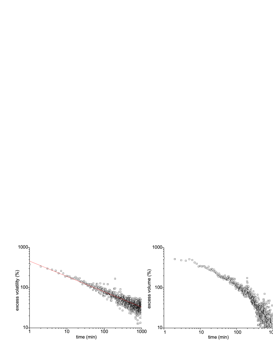
Table 6: Exponent of fitted power-law decay for volatility

Post-event evolution of excess volatility during the first 1000 minutes can be well fitted by a power-law. The reported exponents are those obtained by simple OLS on minute data for different filter parameters on both markets for both increases and decreases.
relative filter 8 6 10 8 8 absolute filter 4 2 6 4 4 event length 60 60 60 10 120 NYSE up -0.27 -0.33 -0.40 -0.31 -0.25 NYSE down -0.35 -0.25 -0.38 -0.31 -0.34 NASDAQ up -0.37 -0.35 -0.41 -0.39 -0.37 NASDAQ down -0.32 -0.35 -0.32 -0.38 -0.40 Mean errors are all below 0.01

Table 7: Power exponent of the decay of autocorrelation of volatility

Measured for some of the most liquid NYSE stocks (Jan. 2000–Sep. 2002) between 1–1000 minutes symbol name power exponent GE General Electric $-0.180\pm 0.015$ AOL AOL Time Warner $-0.171\pm 0.014$ C Citigroup Inc. $-0.138\pm 0.016$ HD Home Depot $-0.160\pm 0.019$ T AT&T Corp. $-0.183\pm 0.019$ IBM Int’l Business Machines $-0.157\pm 0.024$ NOK Nokia $-0.202\pm 0.015$

The decrease of post-event excess volatility can in fact be well fitted by a power-law as shown in Figure 3. On the other hand it ce=an be inferred from the figure that the decay of excess volume cannot be described by a power-law. Graphical analysis reveals that none of the variables decay exponentially. We measure the exponent of the power-law for the both markets for a variety of filter levels. From Table 6 we can conclude that the exponent is between 0.25-0.35 on the NYSE and 0.35-0.40 on the NASDAQ. In the vast majority of the cases the power-law gives a very good fit. As we have already done for a small number of filter levels (?) we can compare the exponent of decay with that of the decay of the autocorrelation of volatility. ? show that the autocorrelation of volatility decays according to a power-law with an exponent of -0.3, pointing out at the same time that the exponent is lower for the first 1000 minutes. Since the authors do not report results for the decay of autocorrelation during the first 1000 minutes (only results from detrended fluctuation analysis) we compute the exponent of the power-law decay for some selected stocks using the same method as ? on data from 2000-2002. The results are presented in Table 7 showing that extreme events decay faster than the autocorrelation. A possible explanation is that large shocks are more likely to be exogenous than all fluctuations incorporated in the ACF (?).

In case of the bid-ask spread on the other hand, which is a major source of transaction costs, we find that it stays virtually unchanged on the NASDAQ but increases to six times its pre-event value on the NYSE (decreasing according to a power-law too). This fact, although in full agreement with the finding of ? that the bid-ask spread does not vary substantially on the NASDAQ during the trading day, implies that a contrarian strategy following the extreme price change has much lower costs on the NASDAQ than on the NYSE.

Figure 4: Evolution of minute volatility, minute dollar volume, and the bid-ask spread on the NYSE and the NASDAQ after intraday price decreases exceeding 4% and 8 times the pre-event volatility

Events are maximum 60-minute long price drops exceeding 4% and 8 times the average 60-minute volatility of the same time interval of the 60 pre-event days. Minute volatility, minute volume and the bid-ask spread are given as a percentage of the 60 pre-event day average of the same minute during the day. An average of 222 events on the NYSE and 215 on the NASDAQ. All events in one sample are at least $T=60$ minutes from each other.

2.4 Profitability of contrarian strategies

To test weak-form market efficiency we have to check whether the large and highly significant reversals on both markets are exploitable, i.e. whether a contrarian strategy yields abnormal profits. Indeed if we calculate the abnormal profit a contrarian trading strategy may achieve during the post-event 30-60 minutes by buying at the ask price at minute 0 and selling at the bid half to one hour later it is significant on both markets (Table 8).

Table 8: Intraday profitability of contrarian strategies

Profitability of buy and hold for 60 minutes strategies. Buying price is the best ask price, selling price the best bid price.
minutes NASDAQ 60-min NASDAQ 120-min NYSE 60-min NYSE 120-min 0-30 1.300%** 2.093%** 0.441%* 0.744%** t-stat (3.24) (3.11) (2.18) (2.85) 0-60 1.599%** 2.686%** 0.439% 0.919%** t-stat (3.87) (4.02) (1.53) (2.50) 2-60 1.268%** 2.149%** 0.257% 0.695%* t-stat (3.84) (4.17) (0.92) (1.94)

* Indicates mean significantly different from zero at the 95% level.

** Indicates mean significantly different from zero at the 99% level.

Omitting all other transaction costs, except for the bid-ask spread, the a trader following a contrarian strategy achieves significant profits on the NASDAQ: after 120-minute price drops 2.686% (4.02) as average of 159 events during the time period 2000-2002. The profits are lower – or in some cases even insignificant – in case of the NYSE because of the widened bid-ask spread. One may argue that these profits can only be acquired by traders who are amazingly fast, but that is not the case. If the trader implementing the contrarian strategy is relatively slow and is only able to buy the stocks two minutes after the event he still receives a profit of 2.149% (4.17) between minutes 2 and 60 on the NASDAQ. Since no events included in the sample happen after one hour before market closure these profits are realized in one hour within the trading day, thus they are unlikely to be seriously affected by mismeasurement of risk. Other trading costs paid by brokers on the NASDAQ are probably not high enough to eliminate these abnormal profits. One must however state that the amount of gain may be limited because limited number of shares are available at the best bid and the best ask price, but profits are significantly larger than 0 (even if not of great absolute value). Further research using the order book at the whole depth and looking at the contracts offered by liquidity providers to their customers may reveal the exact profit which can be achieved by the above trading strategy.

The number of stocks which pass the liquidity filter, i.e. the number of stocks which have to be tracked each day during the trading, is 101-144 for the NASDAQ and 47-252 for the NYSE. Sophisticated trading software can in theory monitor this number of stocks throughout the day signaling when an event has taken place, when to buy and when to sell. Further studies should examine the exact profitability, if any, of such strategies taking into account all other costs of transaction and the costs of monitoring the prices of liquid stocks.

3 Conclusions

In our empirical study we examine the price of liquid stocks after experiencing a large 60-minute price change using data from the NYSE and the NASDAQ. Focusing on short-term reaction we find significant overreaction on both markets in the subsequent 30-60 minutes. Stability analysis confirms our findings. This implies there is a short-term market inefficiency which we name ”intraday reversal puzzle”. and one of the main goals of our paper is to call the attention to this empirical fact. Presently, we can only speculate about the origin of this phenomenon. It may be due to behavioral trading during the period of rapidly changing price or to some kind of interaction between informed and uninformed traders. We show that the size of the reversal is positively dependent on the initial price change and compatible with a linear assumption, at least for not too large changes.

An interesting aspect is the very different behavior of the bid-ask spread on the NYSE and on the NASDAQ close to a major price change: an enormous increase is observed on the former, while practically no significant change accompanies the event on the latter (cf. Fig. 4). The origin of this has to be rooted in the different market mechanisms, and we believe that the explanation is somewhat paradoxical. On the NYSE where a single specialist acts, he/she eliminates a large part of the profit a contrarian strategy may achieve by simply widening the bid-ask spread. At the same time, the highly competitive dealership market on the NASDAQ keeps the bid-ask spread almost constant, thus giving way to a short-term abnormal profit possibility.

In case of extreme price changes we find that intraday contrarian trading strategies are profitable even after controlling for the bid-ask spread. Exact profitability of such strategies should although be studied further by taking into account further sources of market friction.

Furthermore we can conclude that volatility, volume, and in case of the NYSE the bid-ask spread, which increase sharply at the event, stay significantly high long after the price adjustment has taken place. In fact the post-event decay of excess volatility (and in case of the NYSE the bid-ask spread) can be well described by a power-law. Comparing the exponent with that of the autocorrelation we can conclude that extreme price shocks decay faster than price fluctuations on average.

Appendix A Possible biases when calculating the average

When averaging the events, we used a minimum distance T between two events included in the sample. In this subsection we address the importance of this issue using a GARCH(1,1) model of minute index data. The equations of the process are:

$$x_{t+1}=x_{t}+\eta_{t+1}$$

$$\sigma_{t+1}^{2}=\alpha_{o}+\alpha_{1}(x_{t}-x_{t-1})^{2}+\beta_{1}\sigma^{2}_{t}$$

$$\eta_{t+1}\in N(0,\sigma_{t+1})$$

where $\alpha_{o}$, $\alpha_{1}$, and $\beta_{1}$ are the parameters of the process. We model the minute price evolution of the market using the following parameters measured on General Electric on the NYSE during the years 2000-2002. Parameters are estimated on the time series of daytime-adjusted returns (daytime averages are measured on the full three-year period) for 295120 data points. The measured parameters using EVIEWS econometrics software package are: $\alpha_{o}=0.0168$, $\alpha_{1}=0.0663$, and $\beta_{1}=0.933$. Thus one time-step of the simulation corresponds to one minute in case of real-market data.

We investigate relatively small sample (150 events) t-tests for the significance of returns in this time series model. In Table 9 we present returns around one minute price drops of at least 8 (which corresponds to 8 times the usual minute-volatility during the same period of the day) with a minimum distance of $T=60$. With this trigger value we get sample events every 403.7 time steps (minutes) which is in the order of magnitude of that measured on real data (e.g. 356 price drops included in the average in 3 years trading time on the NASDAQ). A GARCH(1,1) process does not exhibit serial correlations (that is why we choose one-minute price drops in the case of the model), thus in theory no reversal may take place and no pre-event drops or increases either. Any significant price patterns measured are due to sample selection bias.

Table 9: The effect of cross sample correlations on significance tests in a model simulation using a GARCH(1,1) process

Average of $1000*150$ price drops of a GARCH(1,1) process with a distance of at least $T=60$ between sample events. Returns and t-values are that of the overall averages. T-average is the average of t-values, abs(t) average of the absolute t-values of 1000 samples of 150 events each. PS is the percentage of small (150 event) samples where t-value indicates significant deviation from zero return at the confidence level of 98%. In case of uncorrelated sample events this value should be $PS\approx 2\%$.

time		return	(t-value)	t-average	abs(t) average	PS
from	to
-181	-121	-0.186	(-1.28)	-0.065	0.812	1.9%
-121	-61	-0.439**	(-2.93)	-0.133	0.812	2.6%
-61	-1	8.72**	(56.20)	2.05	2.07	37.8%++
-1	0	-10.76**	(-789.6)	-39.5	39.5	100.0%++
0	10	0.00942	(0.145)	0.009	0.812	2.4%
0	60	-0.0132	(-0.085)	-0.013	0.799	1.7%
60	120	-0.172	(-1.13)	-0.062	0.824	2.4%
0	390	-0.0175	(-0.047)	-0.034	1.771	29.3%++
0	1000	-0.599	(-1.094)	-0.035	2.492	46.3%++

** Indicates large sample mean return significantly different from 0 at the 99% level.

⁺⁺ Indicates PS significantly different from 2% at the 99% level.

It can be inferred from the data that calculated t-statistics for returns during longer time periods than T are biased (although the returns themselves are not). Because of the spurious cross-sample correlation we get a t-value indicating significant deviation (at the 98% level using a two-sided test) from the fact that returns are zero in much more than 2% of the cases (see last column in Table 9). Thus returns on real-market data of time periods longer than T should not be tested by the t-statistics. This holds even if we investigate overlapping time windows of different stocks because their returns are correlated as well. When daily (close-to-close) price drops are examined we may get strong cross-sample correlations if we include more than one event on one particular day in our sample thus the t-values calculated by e.g. ? may be biased. Our results show furthermore that the t-values computed by ? and ? showing significant long-term reversals (of the length of 3-17 days) should be considered with care as well, although significance of daily returns shown in these studies are not affected by this problem, and are to be accepted.

Another result we obtain from the model data is that pre-event returns are biased. Using the above sample selection process we get returns significantly different from zero before the event. This is due to the fact that during the last T minutes of the pre-event period all events (i.e. large decreases) are excluded but large increases are included: thus we have returns biased toward price increases. The reason why this effect is so strong is that the GARCH(1,1) process similarly to the real-market data exhibits volatility clustering, i.e. large price decreases and increases tend to cluster which only increases the number of excluded pre-event large price decreases. It is most probable that the sharp decline in price preceding intraday price jumps in our results as shown in Table 1 and on Figure 1 are due to this effect. This bias on the other hand should lead to a similar price increase before intraday price drops, which however cannot be observed; showing a strong asymmetry between the pre-event market sentiment in case of large intraday increases and decreases. Price drops seem thus to be preceded by strong selling.

Notes

¹Intraday market reaction for index futures following large price changes at the opening of the market is analyzed by ?. However, the small amount of data existing for index futures only allows the investigation of small price changes, thus the conclusions are not robust.

² Overreaction is found on other markets as well: ? find significant overreaction on the TSE (Tokyo Stock Exchange), and ? in Johannesburg.

³See e.g. ?; ?; ?.

⁴See e.g. ?; ?; ?; ?.

⁵The first trading minute according to this methodology is usually between 9:30 and 9:35. Some trading occurs after 16:00 but it is omitted for convenience.

⁶The opening second of the NASDAQ is 9:30:00 and the closing is 16:00:00 ET.

⁷This daytime adjustment of volatility is based on the idea of ?

⁸Intraday index data is that of Disk Trading Ltd.