Critical properties of random anisotropy magnets

Abstract

The problem of critical behaviour of three dimensional random anisotropy magnets, which constitute a wide class of disordered magnets is considered. Previous results obtained in experiments, by Monte Carlo simulations and within different theoretical approaches give evidence for a second order phase transition for anisotropic distributions of the local anisotropy axes, while for the case of isotropic distribution such transition is absent. This outcome is described by renormalization group in its field theoretical variant on the basis of the random anisotropy model. Considerable attention is paid to the investigation of the effective critical behaviour which explains the observation of different behaviour in the same universality class.

, ,

1 Introduction

The influence of structural disorder on the critical behaviour remains to be one of the most attractive problems of phase transitions theory [2]. It is known that even small disarrangement in the structure of ideal physical systems may have crucial consequences for their behaviour near a critical point [3, 4]. In particular, weak quenched disorder in magnetic systems can not only change the characteristics of the second order phase transition or the order of the phase transition into the low-temperature phase, it can modify also the nature of this phase, producing spin-glass order. Among disordered magnets depending on the type of randomness of their structure random site [3, 4], random field [5], and random anisotropy [6] systems can be discriminated. All these magnets were extensively investigated, however, in our view, less attention was paid to the critical behaviour of the last class of systems i.e. random anisotropy magnets, in particular to random anisotropy effects on second order phase transitions. This motivates us to present an analysis of the problem by the field-theoretical renormalization group (RG) methods [7], which are standard for studying the second order phase transition of ideal systems; we also briefly review the present state of the investigations of the low-temperature phase of the random anisotropy magnets. The main goal of our study is to emphasize the crucial role played by distribution of the random axes in defining the university class of random anisotropy magnets, and hence the very possibility of a second order phase transition and its scenario. Moreover, in our study we will address the effective behaviour of random anisotropy magnets: it is frequently encountered in experimental and MC studies but less attention has been paid to it in the theoretical analysis.

The paper is organized as follows: in the next Section we give a review of experimental, numerical and theoretical analysis of the low-temperature phase in random anisotropy magnets. Since we apply in our study the field-theoretical RG, Section 3 discusses the functional representation of the model of a random anisotropy magnet for different types of distributions of the local anisotropy axes as well as the stability conditions for the effective Hamiltonians. Section 4 presents the application of the field-theoretical RG approach to study the critical behaviour of the random anisotropy model (RAM). There, the RG functions are obtained in the two-loop approximations within the minimal subtraction scheme. The analysis of the asymptotic and the non-asymptotic critical behaviour is performed using the resummation techniques in space dimension $d=3$. Section 5 concludes our study and summarizes the results.

2 A brief review of earlier experimental, numerical, and theoretical studies

Magnetic properties of random anisotropy magnets are described by the RAM [8]. This is a spin lattice model with each spin subjected to a local anisotropy of random orientation. The Hamiltonian reads:

$${\mathcal{H}}=-\sum_{{\bf R},{\bf R^{\prime}}}J_{{\bf R},{\bf R^{\prime}}}\vec{S}_{\bf R}\vec{S}_{\bf R^{\prime}}-D\sum_{{\bf R}}(\hat{x}_{\bf R}\vec{S}_{\bf R})^{2}.$$ (1)

Here, $\vec{S}_{\bf R}$ is a classical $m$–component vector (“spin”) on the site ${\bf R}$ of a $d$–dimensional (hyper)cubic lattice, $D>0$ is the strength of the anisotropy, $\hat{x}_{\bf R}$ is a random unit vector pointing in the direction of the local anisotropy axis. The interaction $J_{{\bf R},{\bf R^{\prime}}}$ is assumed to be ferromagnetic. For the short-range case it can be written in form of the nearest-neighbours interaction:

$$J_{{\bf R},{\bf R^{\prime}}}=\left\{\begin{array}[]{cc}\bar{J}>0,&\quad|{\bf R}-{\bf R^{\prime}}|=a;\\ 0&\quad\mbox{otherwise},\end{array}\right.$$

where $a$ is the distance between the nearest neighbours. The degree of disorder is controlled by the ratio $D/{\bar{J}}$. Obviously, the random orientations are present in (1) only for $m>1$. In the case $m=1$ the random anisotropy term becomes constant and leads only to a shift of the Ising system free energy.

The RAM (1) is relevant to describe a wide class of disordered magnets. It was first introduced to describe magnetic properties of amorphous alloys of rare-earth compounds with aspherical electron distributions and transition metals [8]. Today the majority of the amorphous alloys including rare-earth elements is recognized to be random anisotropy magnets. This class of amorphous materials includes binary alloys [9, 10, 11, 12, 13, 14, 15], alloys of rare earths with two metallic components [16, 17, 18, 19, 20, 21, 22, 23, 24, 25], alloys of rare earth with a metal and a non-metallic component [26, 27, 28, 29, 30] and multicomponent alloys [31, 32, 33, 34, 35, 36]. The structure of these compounds is characterized by an uniform (isotropic) distribution of the direction of the random anisotropy axes. Also crystalline compounds such as $RE_{x}Y_{1-x}Al_{2}$ $(RE=Tb,\,Dy)$ [37, 38, 39, 40, 41, 42, 43] are described by the RAM. However in this case, a distribution of the random anisotropy axes orientations is confined to several directions only. It turned out that random anisotropy plays a distinguished role also in the magnetic behaviour of certain uranium based amorphous alloys [44, 45, 46]. Although all materials mentioned above represent the case of spin dimension $m=3$, certain magnets are described by the RAM with $m=2$ [47, 48].

Beside traditional magnets, random anisotropy is present in such magnetic materials as molecular based magnets [49], nanocrystallity materials [50] and granular systems [51].

The problem of the nature of a low-temperature phase of random anisotropy magnets and peculiarities of the transition to this phase was investigated extensively by theoretical approaches, numerical simulations and experiments. Below we summarize what has been obtained so far for the three dimensional systems. In a separate subsection, we mention also some results for the RAM at lower dimensions.

2.1 Experiments

The earliest experimental data about amorphous alloys containing rare earth and transition metals are collected in the comprehensive review of Cochrane et al. [6]. Results of later experimental investigations are reviewed in the paper of Sellmyer and O’Shea [52]. Most of the investigated materials was recognized as systems with strong anisotropy. For many of them in the low-temperature phase an extremely large magnetic susceptibility was observed which was consistent with theoretically predicted peculiarities [53]. However no phase with a non-zero magnetization was obtained. The majority of investigations of amorphous random anisotropy systems reports the low-temperature phase to be either a spin-glass phase or a so called correlated spin glass phase, in terms of the phenomenological theory [54] often used for the interpretation of data.

Most of the examples given above concern systems with an isotropic distribution of the orientation of the random anisotropy axes. However the crystalline compounds $RE_{x}Y_{1-x}Al_{2}$ $(RE=Tb,\,Dy)$ [37, 38, 39, 40, 41, 42, 43] are examples of random anisotropy systems, where the distribution of local anisotropy axes is anisotropic. The rich phase diagram of these systems contrary to isotropic alloys presented evidence of a ferromagnetic phase for very weak anisotropy [39].

Therefore the experiments indicate the absence of a ferromagnetic phase for amorphous systems in general, with the possibility of ferromagnetism for crystalline compounds with weak random anisotropy. The effective critical behaviour of random anisotropy magnets was not considered. The question about effective critical exponents was touched only in Ref. [55], where the temperature region of asymptotic critical regime was discussed for random anisotropy magnets.

2.2 Monte Carlo simulations

The majority of the computer simulations exploiting the RAM concerned the case of strong ($D/{\bar{J}}>>1$) or more often infinitely strong anisotropy ($D/{\bar{J}}\to\infty$). The earliest investigations report inconclusive results: both stability [56, 57] as well as instability [58, 59] of the ferromagnetic order with respect to the spin-glass phase has been reported. However, data of later investigations indicated the absence of ferromagnetism. The restriction to the infinitely strong anisotropy limit led to a lack of long-range order in the ground state for $m=3$ [60]. In this limit, the critical exponents at the transition to a low-temperature phase were found to be similar to those of the three-dimensional short-range interacting Ising spin glass [61]. The results of Monte Carlo calculations [62, 63] confirmed an absence of ferromagnetism.

On the other hand, Monte Carlo results for the RAM with $m=2$ are consistent with the existence of a low-temperature phase of extremely large susceptibility [62]. This feature was predicted theoretically for arbitrary $m$ and weak anisotropy [53]. The possibility of the existence of such a phase was indicated also in investigations of spin models with $p-$fold random fields [63], which in the case $m=2$, $p=2$ correspond to the RAM with $m=2$.

Monte Carlo simulations for $m=2$ show also the existence of a non-magnetic low-temperature phase with power-law decay of a pair correlation function predicted for the RAM [53]. The result [64] for infinite anisotropy is consistent with this quasi-long-range ordered phase. On the other hand such phase was not obtained for the model with $p-$fold fields at $\bar{J}=D$ [65]. Moreover, another Monte Carlo study of the RAM with $m=2$ and the same relation between $\bar{J}$ and $D$ obtained critical exponents with values similar to the $XY$-ferromagnetic transition, except that the heat capacity critical exponent was found to be positive [69]. It was shown that the long-range order is not destroyed in the vortex-free model with $p-$fold fields [68].

The possibility of the existence of a quasi-long-ordered phase was also obtained for $m=3$ in the case of weak anisotropy but assuming $D/\bar{J}=\infty$ for a part $q$ of sites and $D/\bar{J}=0$ for the rest of $1-q$ sites [66]. Here, the quasi-long-range ordered phase appeared as an intermediate phase between the paramagnetic and the ferromagnetic ordering. However, for a non-zero anisotropy $D$ the low temperature phase appears to be a quasi-long-range one [67].

To our knowledge, there exists only one the Monte Carlo study for the random axis anisotropic distribution. This is a study of a cubic model with random anisotropy, where the anisotropic axes are oriented along the edges of a cube [70]. For $m=2$ the conventional XY second order phase transition to the ferromagnetic phase was found for weak random anisotropy, whereas a first-order transition to a domain type ferromagnetic phase was found for strong random anisotropy. For $m=3$ both transitions were found to be of the first order.

Therefore, although there is a certain inconsistency of Monte Carlo results, they mainly confirm the experimentally observed absence of ferromagnetism for random anisotropy magnets with isotropic distribution of random axes and bring about a second order phase transition for the weak randomness with anisotropic distribution. However, a low-temperature phase with power-law decay of correlation functions as observed in Monte Carlo simulations has not been found in the experiments so far.

2.3 Theoretical treatment

The first theoretical investigations of the RAM were performed within a mean field theory. Ferromagnetism was predicted [8, 71] but the possibility of a spin-glass phase [72] was not excluded. Within the mean field approach the infinite-range interaction limit of the RAM was solved exactly [73], indicating a second-order phase transition to ferromagnetic order.

However, taking into account fluctuations lead the second order phase transition disappeared. In the pioneer RG calculations performed for RAM with isotropic distribution of $\hat{x}_{\bf R}$ [74] no stable accessible fixed point of the RG transformation was found within the first order of $\varepsilon=4-d$-expansion. Recently, this result was corroborated by two-loop [75, 76, 77] and even five-loop [78] calculations within the field-theoretical RG refined by resummation techniques. Meanwhile, an effective free energy was derived for large $D$. It was shown to have the same form as that of the random-bond Ising spin glass [79], demonstrating that the RAM can have a spin glass phase. Following the arguments of Imry and Ma [80] formulated for the random-field model it was shown that the $d=3$ random anisotropy magnet should break into magnetic domains of size $L\sim(\bar{J}/D)^{2}$ [81] for weak anisotropy and thus no ferromagnetism was expected. Several different arguments were applied to the RAM [82] in order to demonstrate the absence of ferromagnetic order for space dimensions $d<4$. Although among these arguments the one for the limit $m\to\infty$ [82] appeared to be erroneous [83], the lack of a ferromagnetism for the RAM with isotropic distribution of anisotropy axes for $d<4$ was further supported by a Mermin–Wagner type proof using the replica trick [84]. The same result was obtained within the Migdal–Polyakov RG technique [85] avoiding the application of the replica trick.

Investigating the equation of state of the RAM a zero magnetization and an infinite magnetic susceptibility were obtained in the low-temperature phase for any $m$ [53]. Two-spin correlations in this phase possess a power law decay. As mentioned above, the phase with such a behaviour is called quasi-long-range ordered. The estimate of the susceptibility of low-temperature phase was corrected in another paper [86] and found to be finite with $\chi\sim(D/\bar{J})^{-4}$ at $d=3$. A similar dependence of the susceptibility was obtained by other approaches [87, 54]. The power law decay of spin correlations in the low-temperature phase was corroborated in particular for $m=2$ [88]. But the last result is in disagreement with calculation results of Ref. [89], where spin-glass phase was obtained. Applying the functional renormalization group in $4-\varepsilon$ dimensions [90, 91] to the RAM with $m=3$, quasi-long-range order was found.

Investigations of the RAM in the spherical model limit $m\to\infty$ were concentrated on the question about the possibility of a spin glass phase. In this limit a ferromagnetic order was obtained for $d>2$ and for $D$ less than some critical value $D_{c}$, while for $D$ larger $D_{c}$ a spin glass phase was obtained for arbitrary $d$ ($D_{c}=0$ for $d\leq 2$) [92]. For these investigations also the $1/m$-expansion [87, 93, 94, 95] was used. Applying the replica method a spin glass phase was found to exist below $d=4$ for arbitrary $D$ [87]. But this spin glass solution later was shown to be unstable [93]. A stable spin glass phase for $d<4$ was obtained avoiding the replica method [94]. However, the dynamics of spin glass order parameter for the RAM showed an instability of the spin glass phase [95]. These results found their confirmation in the mean field treatment of the $m\to\infty$ limit [96], where the spin glass phase appeared only as a feature of this limit and no spin glass phase was obtained for finite $m$.

The phenomenological theory [54] based on the continuous version of the Hamiltonian (1) and assuming correlations between randomly oriented anisotropy axes turned out to be a more appropriate approach for the interpretation of the field dependence of the experimentally observed magnetization in the ordered phase. In this approach the spin correlation functions in different regimes of applied fields were analyzed [54]. In particular, the correlation length for small and zero fields was found to have the form $\xi\sim R_{a}(\frac{\bar{J}}{R_{a}D})^{2}$, where $R_{a}$ is the correlation range for random axes. Such a phase was called a correlated spin-glass phase.

The infinitely strong anisotropy limit of the RAM was investigated with the help of high-temperature expansions. Results of a Padé-analysis [97] indicated typical spin glass behaviour for space dimension $d=3$, while in Ref. [98] it was concluded that the lower critical dimension for the RAM with $m=2$ is $d_{L}=3$. The high-temperature series analysis of the Hamiltonian (1) on Cayley-trees [99] predicted ferromagnetic order, occurring for the number of nearest neighbours $\tilde{z}>m$ and a spin glass order for $\tilde{z}<m$.

All theoretical approaches summarized above concerned the RAM with isotropic random axes distribution. The anisotropic case was first investigated in a RG study [74] with a distribution of anisotropic axes, restricting directions of the axes along the hypercube edges (cubic distribution). No accessible stable fixed point corresponding to a second order phase transition point was found. Investigating the RAM with mixed isotropic and cubic distributions it was found [100] that the presence of a random cubic anisotropy stabilizes the ferromagnetic phase. The possibility of a second order phase transition into a ferromagnetic phase with critical exponents of the diluted quenched Ising model for the RAM with a cubic distribution was pointed out in Ref. [101]. Such a behaviour was observed for a more general model [102] containing non-isotropic terms. It included the RAM with cubic distribution of random axes as a particular case. Subsequently, this result was corroborated within a two-loop RG calculations with resummation [76, 77, 103] done directly for the RAM and it was shown that the critical behaviour belongs to the universality class of the site-diluted Ising model. This result was further confirmed on the basis of a five-loop massive RG calculations [78].

2.4 RAM at low dimensions

It is interesting to compare the above mentioned results with those for low-dimensional random anisotropy systems. For $d{=}2$ both theoretical approaches [104] and numerical simulations [105] lead to a spin-glass character of the low-temperature phase. An exception was a functional RG investigation [106] showing the instability of the ferromagnetic order and a logarithmically slow decrease of the correlation functions.

Results for the RAM in $d=1$ dimensions do not give such a consistent picture. Investigations of the $d=1$ infinity anisotropy limit [107] gave a spin-glass ground state. However, a Monte Carlo investigation for finite $D$ [108] was unable to find a ground state with zero magnetization. While another numerical study [109] demonstrated a decrease of the correlation length with $D$. Monte Carlo simulations [110] indicated a zero temperature magnetization.

2.5 Some conclusions

As one can see from the picture described above there exists a contradictory results concerning the transition of the random anisotropy magnets into the low-temperature phase. The majority of the results state that the $d=3$ RAM has no low-temperature phase with non-vanishing magnetization for the isotropic distribution of the local anisotropy axes. Investigations of the RAM with an anisotropic distribution of the anisotropy axes bring about the possibility of a ferromagnetic phase. Theory predicts a power-low decay of correlation functions in the low-temperature phase, which is confirmed by Monte Carlo simulations, however no phase with such features was observed in experiments. The question of effective critical behaviour of random anisotropy magnets remains unclear.

Nowadays the field-theoretical RG approach serves as a reliable method to get accurate results describing critical behaviour [7]. For the RAM, only the papers [74, 75, 76, 77, 78, 101, 103] were devoted to such analysis. They concentrated on the study of the asymptotic critical behaviour of the RAM. Below we will consider results of these studies in more details, revisiting the $d=3$ RAM criticality within the minimal subtraction RG scheme. Doing so, we will study the effective critical behaviour of the random anisotropy magnets. It is this non-asymptotic critical behaviour that often is observed in experiments and Monte Carlo simulations of critical systems near second order phase transition. The analysis of the asymptotic and non-asymptotic critical behaviour is carried out in the Section 4, while in the next Section 3 the effective Hamiltonians for RAM with isotropic and cubic distributions of local axes are discussed.

3 Effective Hamiltonians for random anisotropy systems

The starting point for an RG analysis of the critical behaviour of the spin model (1) is an effective Hamiltonian, derived for a given random axes $\{\hat{x}_{\bf R}\}$ distribution. The functional representation of the RAM and hence the effective Hamiltonian can be obtained using symmetry considerations [74, 78], however it can be obtained also directly starting from the original spin Hamiltonian (1). Along the line of derivation, it will become clear, how the random axes distribution influences the symmetry of the effective Hamiltonian and hence defines the universality classes of our problem. The details of this procedure based on the Stratonovich-Hubbard transformation are given in the Appendix.

The case we consider here corresponds to the non-equilibrium disorder [111]: variables $\hat{x}_{\bf R}$ in (1) are randomly distributed and fixed (quenched) in a certain configuration. As derived in the Appendix, the configuration-dependent partition function $Z(\{\hat{x}_{\bf R}\})$ for the case of weak anisotropy $D/\bar{J}<<1$ reads:

$$Z(\{\hat{x}_{\bf R}\})\sim\int(d\vec{\phi})e^{{\mathcal{H}}(\hat{x}_{\bf R},\vec{\phi}_{\bf R})},$$ (2)

where the integral means functional integration in the space of the $m$-component fields $\vec{\phi}_{\bf R}=({\phi}^{(1)}_{\bf R}\dots{\phi}^{(m)}_{\bf R})$ and the Hamiltonian ${\mathcal{H}}({\hat{x}_{\bf R},\vec{\phi}_{\bf R}})$ reads:

$${\mathcal{H}}({\hat{x}_{\bf R},\vec{\phi}_{\bf R}}) = -\int d^{d}R\Big{\{}\frac{1}{2}\left[r_{0}|\vec{\phi}_{\bf R}|^{2}+\left|\vec{\nabla}\vec{\phi}_{\bf R}\right|^{2}\right]{-}D_{1}\left(\vec{\phi}_{\bf R}\hat{x}_{\bf R}\right)^{2}{+}v_{1}|\vec{\phi}_{\bf R}|^{4}+$$ (3)

$$z|\vec{\phi}_{\bf R}|^{2}\left(\vec{\phi}_{\bf R}\hat{x}_{\bf R}\right)^{2}+\dots\Big{\}}.$$

Here, $r_{0}$ is proportional to the distance from the critical temperature and $v_{1}$, $D_{1}$, $z$ are positive constants connected to the parameters of the spin Hamiltonian (1) via relations explicitly given in the Appendix.

This form of functional representation differs from the one obtained by symmetry consideration [74, 78] by the presence of the term with coupling $z$, however, as it will be shown below, this term does not affect the critical behaviour of the RAM since the symmetry of the resulting effective Hamiltonian does not change when this term is omitted. In order to obtain the free energy $F$ describing the physical system for the quenched disorder [111] one has to average the logarithm of configuration dependent partition function $Z(\{\hat{x}_{\bf R}\})$ over all possible random configurations $\{\hat{x}_{\bf R}\}$ of the directions of the anisotropy axes:

$$-\beta F=\int\dots\int[d^{m}\hat{x}_{\bf R}]P(\{\hat{x}_{\bf R}\})\ln Z(\{\hat{x}_{\bf R}\}).$$ (4)

Here, $P(\{\hat{x}_{\bf R}\})$ is the probability of a realization of a given configuration $\{\hat{x}_{\bf R}\}$. If one assumes that there are no correlations between the directions of $\hat{x}_{\bf R}$ on different sites, the probability distribution is factorised into a product of distributions $p(\hat{x}_{\bf R})$ of $\hat{x}_{\bf R}$ on each site $\bf R$ :

$$P(\{\hat{x}_{\bf R}\})=\prod_{\bf R}p(\hat{x}_{\bf R}).$$ (5)

To achieve the calculations of the logarithm of the partition function it is convenient to use the replica trick [84] introducing powers of $Z(\{\hat{x}_{\bf R}\})$ which are easier to average:

$$\ln Z(\{\hat{x}_{\bf R}\})=\left.\frac{\partial}{\partial n}\left[Z(\{\hat{x}_{\bf R}\})\right]^{n}\right|_{n=0}.$$ (6)

Now the model must be completed by choosing a certain distribution $p(\hat{x}_{\bf R})$ for the random variables $\hat{x}_{\bf R}$. On the one hand, this distribution should be simple enough from the mathematical point of view, on the other hand, it must contain certain physical constraints. Aharony [74] considered two types of distributions of $\hat{x}_{\bf R}$. The first is an isotropic one, where the random vector $\hat{x}_{\bf R}$ points with equal probability in any direction in the $m$-dimensional hyperspace:

$$p(\hat{x})\equiv\left(\int d^{m}\hat{x}\right)^{-1}=\frac{\Gamma(m/2)}{2\pi^{m/2}}.$$ (7)

Here $\Gamma(x)$ is Euler gamma-function, and the right-hand side presents the volume of the $m$-dimensional hypersphere of unit radius. This distribution mimics an amorphous system without any preferred directions. The second distribution restricts the vector $\hat{x}_{\bf R}$ to point with equal probability only along one of the $2m$ directions of the axes $\hat{k}_{i}$ of a (hyper)cubic lattice:

$$p(\hat{x})=\frac{1}{2m}\sum_{i=1}^{m}\left[\delta^{(m)}(\hat{x}-\hat{k}_{i})+\delta^{(m)}(\hat{x}+\hat{k}_{i})\right],$$ (8)

where $\delta(y)$ are Kronecker’s deltas. This distribution will be called cubic distribution henceforth. The cubic distribution corresponds to a situation when an amorphous magnet still “remembers” the initial cubic lattice structure in spite of the random anisotropy or describes crystalline compounds with random but restricted anisotropy. It is an example of the cases of more general anisotropic distributions.

Performing the average over the random variables $\{\hat{x}_{\bf R}\}$ for the isotropic distribution (7) one ends up with the effective Hamiltonian [74]:

$${\mathcal{H}}_{eff} = -\int d^{d}R\Bigg{\{}\frac{1}{2}\left[\mu_{0}^{2}|\vec{\varphi}|^{2}+\left|\vec{\nabla}\vec{\varphi}\right|^{2}\right]+u_{0}|\vec{\varphi}|^{4}+$$ (9)

$$v_{0}\sum_{\alpha=1}^{n}|\vec{\phi}^{\alpha}|^{4}+w_{0}\sum_{\alpha,\beta=1}^{n}\sum_{i,j}^{m}\phi_{i}^{\alpha}\phi_{j}^{\alpha}\phi_{i}^{\beta}\phi_{j}^{\beta}.$$

It describes in the replica limit, $n\to 0$, the critical properties of model (1) with distribution (7). Here $\mu_{0}=r_{0}-D_{1}/m$ is the bare (non-renormalized) mass and $u_{0}=\frac{D_{1}^{2}}{m^{2}(m+2)}>0$, $v_{0}=v_{1}+z/m>0$, $w_{0}=-\frac{D_{1}^{2}}{m(m+2)}<0$ are the bare couplings. $\phi_{i}^{\alpha}\equiv\phi_{i,{\bf R}}^{\alpha}$ are components of the $n$-replicated $m$-dimensional field, $|\vec{\varphi}|^{2}\equiv\sum_{i}\sum_{\alpha}\left|\phi_{i}^{\alpha}\right|^{2}$. The ratio of the couplings $w_{0}$ and $u_{0}$ equals $w_{0}/u_{0}=-m$ and determines a region of physically allowed initial values in the $(u-v-w)$-space of couplings.

For the cubic distribution (8) the average over the random variables $\{\hat{x}_{\bf R}\}$ leads to the effective Hamiltonian of the following form [74]:

$${\mathcal{H}}_{eff}{=} {-}\!\!\int\!\!d^{d}R\Bigg{\{}\!\frac{1}{2}\!\left[\mu_{0}^{2}|\vec{\varphi}|^{2}{+}\!\left|\vec{\nabla}\vec{\varphi}\right|^{2}\right]\!\!{+}u_{0}|\vec{\varphi}|^{4}{+}v_{0}\!\!\sum_{\alpha=1}^{n}|\vec{\phi}^{\alpha}|^{4}\!{+}$$ (10)

$$w_{0}\!\sum_{i=1}^{m}\!\sum_{\alpha,\beta{=}1}^{n}\left(\phi_{i}^{\alpha}\right)^{2}\left(\phi_{i}^{\beta}\right)^{2}{+}y_{0}\sum_{i=1}^{m}\sum_{\alpha=1}^{n}\left(\phi_{i}^{\alpha}\right)^{4}\!.$$

Again, one has to perform the replica limit $n\to 0$ to get the physical quantities. Here, the bare mass and couplings are determined as: $\mu_{0}=r_{0}-D_{1}/m$, $u_{0}=\frac{D_{1}^{2}}{2m^{2}}>0$, $v_{0}=v_{1}+z/m>0$, $w_{0}=-\frac{D_{1}^{2}}{2m}<0$. The last term in (10) has cubic symmetry. It does not result from the steps leading to ${\mathcal{H}}_{eff}$ but has to be included in (10) since it is generated by further application of the RG transformation. Therefore $y_{0}$ can be of either sign. The symmetries of $w_{0}$ terms differ in (9) and (10). Furthermore, although values of $u_{0}$ and $w_{0}$ differ for Hamiltonians (9) and (10), their ratio again equals $-m$.

It should be noted that for $m=1$ the effective Hamiltonians (9) and (10) reduce to the traditional effective Hamiltonian of the Ising magnet with one coupling, demonstrating the degeneration of the random anisotropy term to a constant for the Ising spins, as mentioned in the introduction. Indeed, in this case the $u_{0}$- and $w_{0}$-terms turn out to have the same symmetry (as well as the $v_{0}$- and $y_{0}$-terms in (10)). Moreover, due to the fixed ratio of these couplings they are equal in their absolute values but have opposite signs and therefore cancel one another. This leads finally to the usual $\phi^{4}$-Hamiltonian.

Other distributions leading to similar effective Hamiltonians as described above are discussed in the Ref. [78]. In particular, let the distribution $p(\hat{x})$, have moments: $M_{i_{1}i_{2}\dots i_{k}}\equiv\int d^{n}x\,p(\hat{x})\,x_{i_{1}}x_{i_{2}}\dots x_{i_{k}}$ satisfying the conditions:

$$M_{ab}=\frac{1}{m}\delta_{ab},\qquad M_{abcd}=A(\delta_{ab}\delta_{cd}+\delta_{ac}\delta_{bd}+\delta_{ad}\delta_{bc})+B\delta_{ab}\delta_{ac}\delta_{ad},$$ (11)

with Cauchy inequalities $A(m+2)+B\geq{1}/{m}$ and $3A+B\geq{1}/{m^{2}}$ for the parameters $A$ and $B$. Then the effective Hamiltonian of the RAM with random anisotropy axis distribution with moments (11) turns out to have the form:

$${\mathcal{H}}_{eff} = -\int d^{d}R\Bigg{\{}\frac{1}{2}\left[(r_{0}-D_{1}/m)|\vec{\varphi}|^{2}+\left|\vec{\nabla}\vec{\varphi}\right|^{2}\right]+v_{0}\!\!\sum_{\alpha=1}^{n}|\vec{\phi}^{\alpha}|^{4}+$$ (12)

$$\frac{D_{1}^{2}}{2m^{2}}(1-m^{2}A)|\vec{\varphi}|^{4}-AD_{1}^{2}\sum_{\alpha,\beta=1}^{n}\sum_{i,j}^{m}\phi_{i}^{\alpha}\phi_{j}^{\alpha}\phi_{i}^{\beta}\phi_{j}^{\beta}-$$

$$\frac{BD_{1}^{2}}{2}\!\sum_{i=1}^{m}\!\sum_{\alpha,\beta{=}1}^{n}\left(\phi_{i}^{\alpha}\right)^{2}\left(\phi_{i}^{\beta}\right)^{2}.$$

However, a term $\sum_{i=1}^{m}\sum_{\alpha=1}^{n}\left(\phi_{i}^{\alpha}\right)^{4}$ has to be added here for the same reason, as it was included in (10). Thus the effective Hamiltonian corresponding to the distribution of $p(\hat{x})$ with conditions (11) reads:

$$\!\!\!{\mathcal{H}}_{eff}{=} \!{-}\!\!\int\!\!d^{d}R\Bigg{\{}\!\frac{1}{2}\!\left[\mu_{0}^{2}|\vec{\varphi}|^{2}{+}\!\left|\vec{\nabla}\vec{\varphi}\right|^{2}\right]\!\!{+}u_{0}|\vec{\varphi}|^{4}{+}v_{0}\!\!\sum_{\alpha=1}^{n}|\vec{\phi}^{\alpha}|^{4}\!{+}$$ (13)

$$w_{0}\!\sum_{i=1}^{m}\!\sum_{\alpha,\beta{=}1}^{n}\left(\phi_{i}^{\alpha}\right)^{2}\left(\phi_{i}^{\beta}\right)^{2}{+}y_{0}\sum_{i=1}^{m}\sum_{\alpha=1}^{n}\left(\phi_{i}^{\alpha}\right)^{4}\!+{z_{0}}\!\!\!\sum_{\alpha,\beta=1}^{n}\sum_{i,j}^{m}\phi_{i}^{\alpha}\phi_{j}^{\alpha}\phi_{i}^{\beta}\phi_{j}^{\beta},$$

Such a Hamiltonian contains symmetry terms of both effective Hamiltonians (9) and (10). It was originally introduced in Ref. [101] to describe magnetic systems with single-ion anisotropy and non-magnetic impurities. The Hamiltonian (13) was studied in the first order in $\varepsilon$ and no accessible and stable fixed point was found [101]. One should note that the $y_{0}$- term in the (12) as well as in (10) appears in a natural way, if one considers the original spin model (1) to contain a cubic symmetry term $\sum_{\bf R}\sum_{i=1}^{m}S^{4}_{i\,\bf R}$.

For distributions with $A=0$ in (11), the effective Hamiltonian (13) reduces simply to (10), since $\tilde{w_{0}}=0$. As it was noted in Ref. [78] this feature is characteristic for all distributions, which orient the anisotropy axis only along the axes of an $m$-dimensional hypercube, including the cases when the anisotropy axis points in positive or in negative directions only.

For the further analysis it is instructive to establish the regions in the space of the coupling constants where the free energy does not diverge in the ordered phase or in other words where the Hamiltonians (9) and (10) are stable. The regions vary for different ordered phases, described by certain nonvanishing values of the order parameter $M$. If one neglects field fluctuations and if the symmetry of the ordered phase is defined by (i) $\phi_{i}^{\alpha}=M$ then the regions of stability for the effective Hamiltonian (9) within the space of couplings are defined by the inequality [101]:

$$v_{0}+nu_{0}+nw_{0}>0.$$ (14)

For the case (ii) $\phi_{i}^{\alpha}=M\delta_{\alpha 1}\delta_{i1}$ the following condition has to be fulfilled [101]:

$$v_{0}+u_{0}+w_{0}>0.$$ (15)

The symmetries (iii) $\phi_{i}^{\alpha}=M\delta_{i1}$ and (iv) $\phi_{i}^{\alpha}=M\delta_{\alpha 1}$ lead to the same conditions (14) and (15) respectively. In a similar way four stability conditions are found [78] for the effective Hamiltonian (10):

$${\rm(i)} \qquad mnu_{0}+mv_{0}+nw_{0}+y_{0}>0,$$ (16)

$${\rm(ii)} \qquad u_{0}+v_{0}+w_{0}+y_{0}>0,$$ (17)

$${\rm(iii)} \qquad nu_{0}+v_{0}+nw_{0}+y_{0}>0,$$ (18)

$${\rm(iv)} \qquad mu_{0}+mv_{0}+w_{0}+y_{0}>0.$$ (19)

As it was argued in Ref. [101], the legitimate stability conditions in the replica limit are those for which isotropy holds in the replica space. Then for Hamiltonian (9) only the inequality (14) is a relevant stability condition, while for Hamiltonian (10) the appropriate conditions are inequalities (16) and (18). In the replica limit they reduce to conditions:

$$v_{0}>0$$ (20)

and

$$mv_{0}+y_{0}>0,\qquad v_{0}+y_{0}>0.$$ (21)

Together with the condition $w_{0}/u_{0}=-m$ the above inequalities (20) and (21) determine all possible initial values of the effective Hamiltonians that can be used in the RG analysis, compared to some expiremental situation or computer simulations.

4 Critical behaviour of the RAM as explained by the renormalization group

In this section the field-theoretical RG approach is applied to analyse critical properties of the RAM. Our previous field-theoretical RG studies exploited the massive renormalization scheme [75, 76, 77, 103] and were restricted to investigation of asymptotic critical properties. Already in the two-loop approximation [75, 76, 77, 103] the critical behaviour was explained, then it was considered again in a five-loop study [78] confirming the former results. Here, we use the minimal subtraction RG scheme within the two-loop approximation to study the effective critical behaviour of the $d=3$ RAM [112]. Since all essential features of asymptotic criticality become evident in this approximation, we consider it to be sufficient for analysing the effective critical behaviour.

4.1 Renormalization

The field-theoretical RG approach [7] is based on the renormalization of one-particle irreducible (1IP) vertex functions defined as

$$\delta(\sum_{i}^{L}p_{i}{+}\sum_{j}^{N}k_{j})\Gamma_{0}^{(L,N)}(\{p\},\{k\},\mu_{0}^{2},\{u_{i,0}\},\Lambda_{0}){=}\int^{\Lambda_{0}}_{0}\!e^{i(\sum_{i}p_{i}r_{i}{+}\sum_{j}k_{j}R_{j})}$$

$$<\!\phi^{2}(r_{1})\dots\phi^{2}(r_{L})\phi(R_{1})\dots\phi(R_{N})\!>_{\rm 1PI}^{{\mathcal{H}}_{eff}}\!dr_{1}\dots dr_{L}dR_{1}\dots dR_{N},$$ (22)

where $\{u_{i,0}=u_{0},v_{0},w_{0},y_{0},...\}$ is a set of bare couplings, $\mu_{0}$ is a bare mass, $\{p\}$ and $\{k\}$ are sets of the external momenta and $\Lambda_{0}$ is the cut-off parameter. The angular brackets in (4.1) denote the statistical average over the Gibbs distribution with the effective Hamiltonian (9) or (10).

The vertex functions appear to be divergent in the infrared limit $\Lambda_{0}\to\infty$. To remove the divergencies, a controlled rearrangement of the perturbative series for the vertex functions is performed. The finiteness of renormalized vertex functions $\Gamma^{(L,N)}$ is ensured by imposing certain normalizing conditions. This leads to different renormalization schemes. In the following, the dimensional regularization with minimal subtraction is used [113].

Normalizing conditions for the minimal subtraction scheme [113] are imposed at zero mass and have the following form:

$$\left.\Gamma^{(0,2)}(k,-k;\tilde{\mu};\{u_{i}\})\right|_{k=0} = 0,$$

$$\frac{d}{d\,k^{2}}\left.\Gamma^{(0,2)}(k,-k;\tilde{\mu};\{u_{i}\})\right|_{k^{2}=\tilde{\mu}^{2}} = 1,$$

$$\left.\Gamma^{(0,4)}_{u_{i}}(\{k\};\tilde{\mu};\{u_{i}\})\right|_{k_{i}{\bf\cdot}k_{j}=\frac{\tilde{\mu}^{2}}{3}(4\delta_{ij}-1)} = \tilde{\mu}^{\varepsilon}u_{i},$$ (23)

$$\left.\Gamma^{(1,2)}(p;k,-k;\tilde{\mu};\{u_{i}\})\right|_{\scriptsize\begin{array}[]{c}p^{2}=k^{2}=\tilde{\mu}^{2}\\ pk=-1/3\tilde{\mu}^{2}\end{array}} = 1.$$ (26)

Here, $u_{i}=\tilde{\mu}^{\varepsilon}\frac{Z_{\phi}^{2}}{Z_{u_{i}}}u_{0}$ are renormalized couplings and $\tilde{\mu}$ is the external momentum scale parameter, $\varepsilon=4-d$. Expansions of the renormalizing factors of the field $\phi$, $Z_{\phi}$, the couplings $\{u_{i}=u,v,w,y,...\}$, $Z_{u_{i}}$, and for the operator $\phi^{2}$, ${\bar{Z}_{\phi^{2}}}$, ensuring finiteness of two-point vertex function with one $\phi^{2}$ insertion, can be obtained from expressions (4.1). The functions $\Gamma^{(0,4)}_{u_{i}}$ are coefficients of terms of different symmetries in the expression for the four-point vertex function $\Gamma^{(0,4)}{}^{ijkl}_{\alpha\beta\gamma\tau}$, containing the full tensorial structure. The last function for the isotropic distribution reads:

$$\Gamma^{(0,4)}{}^{ijkl}_{\alpha\beta\gamma\tau}{=}\Gamma^{(0,4)}_{u}{S}^{ijkl}_{\alpha\beta\gamma\tau}{+}\Gamma^{(0,4)}_{v}{S}_{ijkl}F_{\alpha\beta\gamma\tau}{+}\Gamma^{(0,4)}_{w}{A}^{ijkl}_{\alpha\beta\gamma\tau},$$ (27)

while for the cubic distribution it is given by

$$\Gamma^{(0,4)}{}^{ijkl}_{\alpha\beta\gamma\tau} {=} \Gamma^{(0,4)}_{u}{S}^{ijkl}_{\alpha\beta\gamma\tau}{+}\Gamma^{(0,4)}_{v}{S}_{ijkl}F_{\alpha\beta\gamma\tau}{+}$$ (28)

$$\Gamma^{(0,4)}_{w}{F}_{ijkl}S_{\alpha\beta\gamma\tau}{+}\Gamma^{(0,4)}_{y}{F}_{ijkl}F_{\alpha\beta\gamma\tau},$$

where

$${F}_{ijkl} {=} \delta_{ij}\delta_{ik}\delta_{il},$$

$${S}_{ijkl} {=} \frac{1}{3}\left(\delta_{ij}\delta_{kl}+\delta_{ik}\delta_{jl}+\delta_{il}\delta_{jk}\right),$$

$${S}_{ijkl}^{\alpha\beta\gamma\tau} {=} \frac{1}{3}\left(\delta_{ij}\delta_{kl}\delta_{\alpha\beta}\delta_{\gamma\tau}{+}\delta_{ik}\delta_{jl}\delta_{\alpha\gamma}\delta_{\beta\tau}{+}\delta_{il}\delta_{jk}\delta_{\alpha\tau}\delta_{\beta\gamma}\right),$$

$${A}_{ijkl}^{\alpha\beta\gamma\tau} {=} {S}_{ijkl}{S}_{\alpha\beta\gamma\tau}-{S}_{ijkl}^{\alpha\beta\gamma\tau},$$ (29)

and $\delta_{ab}$ is the Kronecker’s delta.

The renormalized vertex functions satisfy the following homogeneous RG equation [7]:

$$\Big{\{}\tilde{\mu}\frac{\partial}{\partial\tilde{\mu}}{+}\sum_{i}\beta_{u_{i}}(\{u_{i}\})\frac{\partial}{\partial u_{i}}{-}\frac{N}{2}\gamma_{\phi}{+}$$

$$L\left({\bar{\gamma}_{\phi^{2}}}{+}\gamma_{\phi}\right)\Big{\}}\Gamma^{(L,N)}(\{p\};\{k\};\tilde{\mu};\{u_{i}\})=0,$$ (30)

(except for the case $L=2$ and $N=0$) with the coefficients:

$$\beta_{u_{i}} {=} \frac{\partial\,u_{i}}{\partial\ln\tilde{\mu}},$$ (31)

$${\gamma}_{\phi} {=} \frac{\partial\ln Z_{\phi}}{\partial\ln\tilde{\mu}},$$ (32)

$$\bar{\gamma}_{\phi^{2}} {=} -\frac{\partial\ln\bar{Z}_{\phi^{2}}}{\partial\ln\tilde{\mu}},$$ (33)

determining the approach of a system to criticality. The case $L=2$ and $N=0$ fulfils an inhomogeneous equation and renormalizes additively. It is important for calculating the specific heat. Because of the scaling laws two exponent functions ${\gamma}_{\phi}$, $\bar{\gamma}_{\phi^{2}}$ are enough to get all exponents. This also holds for the effective exponents above $T_{c}$ in the approximation we use them here.

The solution of the RG equation (4.1) via the method of characteristics introduces the flow equations:

$$\ell\frac{du_{i}}{d\ell}=\beta_{u_{i}}(\{u_{i}\}).$$ (34)

The flow parameter $\ell$ is related via a matching condition to the distance from the critical point $\tau$. In the limit $\ell\to 0$ the scale-dependent values of the couplings $u_{i}(\ell)$ will approach their stable fixed point (FP) values $\{u^{*}_{i}\}$, if such a FP exists and if it is attainable from the initial values for (34) (initial “background” values of couplings).

The FPs of the system of equations (31) are defined as the set of real zeros of the $\beta$-functions:

$$\beta_{u_{i}}(\{u^{*}_{i}\}){=}0.$$ (35)

A FP is stable if all eigenvalues $\omega_{i}$ of the stability matrix $B_{i,j}=\frac{\partial\beta_{u_{i}}}{\partial{u_{j}}}$ calculated at this FP have positive real parts. A stable FP corresponds to the critical point of the system only if this FP is reachable from physical meaningful initial conditions. The critical exponents are then obtained from the $\gamma$-functions evaluated at this stable FP. The corresponding expressions for the exponent $\nu$ of the correlation length and the exponent $\eta$ of the pair correlation function at $T_{c}$ are expressed by the FP values of the $\gamma$-functions (32), (33):

$$\nu {=} \left[2-\bar{\gamma}_{\phi^{2}}(\{u^{*}_{i}\})-{\gamma}_{\phi}(\{u^{*}_{i}\})\right]^{-1},$$ (36)

$$\eta = {\gamma}_{\phi}(\{u^{*}_{i}\}).$$ (37)

The solution of the RG equation (4.1) together with the solution for vertex function $\Gamma^{(2,0)}$ proof scaling. Therefore, all other critical exponents may be obtained from the familiar scaling laws. For example, the susceptibility exponent $\gamma$ is given by:

$$\gamma{=}(2-\eta)\nu,$$ (38)

and thus expressed by the $\gamma$-functions (32), (33) as:

$$\gamma^{-1}{=}1-\frac{\bar{\gamma}_{\phi^{2}}(\{u^{*}_{i}\})}{2-{\gamma}_{\phi}(\{u^{*}_{i}\})}.$$ (39)

Other exponents are found in a similar way.

4.2 Asymptotic critical behaviour

First, we analyse the asymptotic critical behaviour of the effective Hamiltonians (9) and (10) within the renormalization scheme described above. For this purpose we write down the explicit expressions for the two-loop RG functions. The resulting FPs obtained by solving the system of the equations for the FP (35) are compared with the results of the massive scheme. This is the basic step before studying the effective critical behaviour in the next subsection 4.3.

4.2.1 Isotropic distribution

Imposing the renormalization conditions of the minimal subtraction scheme (4.1) to the vertex functions of the theory with the effective Hamiltonian (9) we found the $\beta$- and $\gamma$-functions within the two-loop approximation (that is within the second and third order in couplings for the $\beta$- and $\gamma$-functions correspondingly):

$$\beta_{u} = {-}u\varepsilon{+}\frac{mn+8}{6}{u}^{2}{+}\frac{m+2}{3}uv{+}\frac{m{+}n{+}1}{3}uw{+}\frac{1}{3}wv{+}\frac{1}{2}{w}^{2}{-}$$ (40)

$$\frac{3mn{+}14}{12}{u}^{3}{-}{\frac{11\left(m+2\right)}{18}}{u}^{2}v{-}{\frac{5\left(m{+}2\right)}{36}}{v}^{2}u{-}$$

$${\frac{\left(5mn{+}5m{+}5{n}+87\right)}{72}}{w}^{2}u{-}{\frac{11\left(m{+}n{+}1\right)}{18}}\!{u}^{2}w{-}$$

$${\frac{5m{+}22}{18}}uwv{-}\frac{m{+}8}{18}{w}^{2}v{-}\frac{m+n+3}{12}{w}^{3}{-}\frac{1}{9}{v}^{2}w,$$

$$\beta_{v} = {-}\varepsilon v{+}\frac{m+8}{6}{v}^{2}{+}2vu{+}\frac{m+5}{3}vw{-}$$ (41)

$$\frac{3m{+}14}{12}{v}^{3}{-}{\frac{11m{+}58}{18}}{v}^{2}u{-}{\frac{17m{+}5n{+}65}{18}}wvu{-}$$

$${\frac{5mn{+}82}{36}}v{u}^{2}{-}{\frac{13m+56}{18}}w{v}^{2}{-}\frac{mn+33m+9n+131}{72}{w}^{2}v,$$

$$\beta_{w} = {-}\varepsilon w{+}\frac{m{+}n{+}4}{6}{w}^{2}{+}2uw{+}\frac{2}{3}wv-$$ (42)

$${\frac{mn{+}3m{+}3n{+}17}{24}}{w}^{3}{-}{\frac{11m{+}11n{+}29}{18}}{w}^{2}u{-}{\frac{5mn+82}{36}}w{u}^{2}{-}$$

$${\frac{m{+}10}{36}}w{v}^{2}{-}{\frac{2\left(m{+}5\right)}{9}}{w}^{2}v{-}{\frac{5m{+}34}{18}}wvu,$$

$$\gamma_{\phi} {=} 0+$$ (43)

$${\frac{m+2}{36}}wv+\frac{m+n+1}{36}uw+\frac{m+2}{36}vu{+}$$

$${\frac{mn{+}m{+}n{+}3}{144}}{w}^{2}{+}\frac{m{+}2}{72}{v}^{2}+{\frac{mn{+}2}{72}}{u}^{2}$$

$$\bar{\gamma}_{\phi}^{2} = \frac{mn+2}{6}u+\frac{m+2}{6}{v}+\frac{m+n+1}{6}w-$$ (44)

$$\frac{mn+2}{12}{u}^{2}-\frac{m{+}2}{6}vu{-}\frac{m{+}2}{12}{v}^{2}{-}\frac{m+2}{6}vw{-}$$

$$\frac{m{+}n{+}1}{6}uw{-}\frac{mn+m+n+3}{24}w^{2}.$$

Here, $\varepsilon=4-d$ and $u,\,v,\,w$ are renormalized couplings. We recall that $m$ is the spin component number and $n$ is the number of replicas. The first line of each formula gives the one loop result in the corresponding RG function. We present the RG functions for any $m$ and $n$, although in the further analysis of the RAM one considers the replica limit $n=0$. However, the effective Hamiltonian (9) for non-zero $n$ may have also other physical interpretations.

An analysis of the RG functions (40)-(44) can be performed in two complementary ways. First, one may apply the $\varepsilon$-expansion [114]. Second, one may fix $\varepsilon$ (i.e. space dimension $d$) in (40)-(44) and solve equations (40)-(42) for the FP numerically [115]. In first order of the $\varepsilon$-expansion, no accessible stable FP was obtained [74]. In second order, calculations performed within the massive scheme [75, 76, 77] did not change this picture qualitatively. Application of the $\varepsilon$-expansion within the minimal subtraction scheme leads to FPs coordinates which, being dependent on the renormalizing conditions [7], differ from those obtained within the massive scheme [75]. The expansions of universal quantities, e. g. critical exponents, coincide in both schemes. Leading to a quantitative information, these expansions for the disordered models [3, 4] in general do not give reliable numerical values for the critical exponents. To give an example, in the case of a random Ising model the expansion turns out to be in $\sqrt{\varepsilon}$, rather then ${\varepsilon}$ [116, 117] and does not lead to reliable estimates at $\varepsilon=1$ ($d=3$) [118]. Therefore we do not display here the results of the expansion in dimension $\varepsilon$ but we discuss in more details the results within the fixed dimension $d$ approach.

The weak-coupling expansions obtained within perturbation theory for the RG functions are asymptotic at best [7]. In order to obtain reliable results one has to apply resummation procedures. Here, the Padé-Borel resummation technique [119] is used. It consists in the following steps. For a given initial polynomial in several variables (in this case in three) for any finite series of $\beta=\beta_{u_{i}}$

$$\beta(u,v,w)=\!\sum_{1\leq i+j+k\leq 3}\!a_{i,j,k}\,u^{i}v^{j}w^{k}$$ (45)

one introduces a “resolvent” polynomial in one auxiliary variable $\lambda$ by [120]:

$$F(u,v,w;\lambda)=\!\sum_{1\leq i+j+k\leq 3}\!a_{i,j,k}\,u^{i}v^{j}w^{k}\lambda^{i+j+k-1},$$ (46)

with the obvious relation $F(u,v,w;\lambda=1)=\beta(u,v,w)$. Then, the Borel image of (46) is defined as:

$$F^{B}(u,v,w;\lambda)=\sum_{1\leq i+j+k\leq 3}\!\frac{a_{i,j,k}{u}^{i}{v}^{j}{w}^{k}\lambda^{i+j+k-1}}{(i+j+k-1)!}.$$ (47)

This truncated series (47) is approximated by the Padé-approximant $[1/1](\lambda)$ [121]. Then, the resummed $\beta$-function is obtained from the formula:

$$\beta^{res}(u,v,w)=\int_{0}^{\infty}dt\exp(-t)[1/1](t).$$ (48)

Applying the above procedure for the analysis of the RG functions (40)-(42) at fixed space dimension $d=3$ and solving the FP equations (35) we get nine FPs. Table 1 lists the FPs for $m=2,\,3,\,4$ in the region of interest: $u^{*}>0$, $v^{*}>0$, $w^{*}<0$. The numeration of FPs corresponds to that of Refs. [74, 75, 76, 77]. FPs V and VII are not listed in the Table 1 since their coordinates are not in the region of interest. Performing the resummation procedure (42)-(45) sometimes one is lead to Padé-approximants containing a pole in the region of integration in (45). Then the principal value of the integral is taken. Coordinates of the fixed points obtained in this way are shown in the Table 1 by small numbers. Some of the FPs in Table 1 correspond to field-theoretical models, relevant for specific physical systems. In particular, FPs II-IV recover results for the isotropic $m$-vector, polymer ($m=0$), and the diluted $m$-vector model correspondingly. All FPs in the Table 1 were already found within the $\varepsilon$-expansion [74]. Their presence was further confirmed by the massive scheme of the field-theoretical RG [75, 76, 77]. Among these FPs only FP III is the stable one, however this FP is not accessible from the initial conditions for the coupling constants.

FP	$m$	$u^{*}$	$v^{*}$	$w^{*}$	$\nu$	$\gamma$
I	$\forall m$	0	0	0	1/2	1
	2	0	1.1415	0	0.684	1.344
II	3	0	1.0016	0	0.720	1.411
	4	0	0.8878	0	0.751	1.470
III	$\forall m$	1.5281	0	0	0.599	1.185
	2	0.1429	0.9923	0	0.665	1.307
IV	3	0.3411	0.6965	0	0.660	1.298
	4	0.4546	0.5323	0	0.656	1.291
VI	2	1.6637	0	-1.8212	0.452	0.911
	3	1.1351	0	-0.9073	0.470	0.944
	2	1.0126	0.9058	-0.6522	0.631	1.243
VIII	3	1.0728	0.7310	-0.5483	0.626	1.235
	4	1.1125	0.6241	-0.4823	0.624	1.230

Table 1: Fixed points and critical exponents $\nu$ and $\gamma$ as obtained on the base of resummed two-loop $\beta$- and $\gamma$-functions for the RAM with isotropic distribution of random anisotropic axes. The only FP III is the stable one.

Table 1 also presents the correlation length critical exponent $\nu$ and the magnetic susceptibility critical exponent $\gamma$ calculated for at the FPs. They are found from expressions $\nu^{-1}=2-\gamma_{\phi}(\{u^{*}_{i}\})-\bar{\gamma}_{\phi^{2}}(\{u^{*}_{i}\})$ and $\gamma^{-1}=1-\bar{\gamma}_{\phi^{2}}(\{u^{*}_{i}\})/(2-\gamma_{\phi}(\{u^{*}_{i}\}))$, which are resummed in the same way as the $\beta$-functions [122].

It should be noted that another stable FP which does not have an analogue among the FPs presented for the massive scheme [75, 76, 77] was found in the region of interest. We do not list the FP in the Table 1 since we consider it uphysical for the reasons explained below. This new FP is not in correspondence with any FP found within $\varepsilon$-expansion [74]. The presence of this FP can be an artifact of the resummation procedure caused by the nonlinearity of the system of the FP equations. Thus, the resummation can lead to the appearance of unphysical FPs. A possible check if a FP makes physical sense can be done by following the dependence of its coordinates on space dimension $d$. If the non-trivial FP at $d=3$ can be traced back to the non-trivial solution at $d=4$ (where the theory is known to contain only the Gaussian FP [7]) this may serve as strong evidence of the unphysical nature of such a FP. However the dimensional dependence of the coordinates of the FP in question could be calculated only up to $d=3.77$, then no real solution can be obtained numerically. Moreover, starting from a certain value of $d$, one has to take principal values of integrals in order to find the FP in the frames of the resummation procedure considered here. A similar problem was observed within two-loop approximation in the massive scheme [75] already at $d=3$. Furthermore, within the five loop order of the massive scheme [78] no evidence for this new stable FP was found. Therefore, we consider this new FP as an unphysical one.

4.2.2 Cubic distribution

Imposing the minimal subtraction renormalization conditions (4.1) to the vertex functions of the theory with the effective Hamiltonian (10) we get the following RG functions in the two-loop approximation:

$$\beta_{u}\! = \!-\varepsilon u{+}\frac{mn{+}8}{6}{u}^{2}{+}\frac{m+2}{3}vu{+}\frac{n+2}{3}uw{+}yu{+}\frac{1}{3}wv{-}$$ (49)

$$\frac{3mn+14}{12}{u}^{3}{-}{\frac{11\left(m+2\right)}{18}}v{u}^{2}{-}{\frac{5\left(m+2\right)}{36}}{v}^{2}u{-}$$

$${\frac{11\left(n+2\right)}{18}u^{2}w}{-}{\frac{5\left(n+2\right)}{36}}u{w}^{2}{-}{\frac{11}{6}}{u}^{2}y-{\frac{5}{12}}{y}^{2}u{-}$$

$$\frac{3}{2}vuw-\frac{5}{6}wyu-\frac{5}{6}vuy-\frac{1}{9}{v}^{2}w-\frac{1}{9}{w}^{2}v,$$

$$\beta_{v}\! = \!-\varepsilon v{+}\frac{m+8}{6}{v}^{2}{+}2vu{+}\frac{2}{3}wv{+}yv{-}$$ (50)

$$\frac{3m+14}{12}{v}^{3}{-}\!{\frac{11m{+}58}{18}}{v}^{2}u{-}{\frac{5mn{+}82}{36}}v{u}^{2}{-}{\frac{n{+}10}{36}}{w}^{2}v{-}$$

$$\!\frac{5}{6}vwy{-}{\frac{31}{18}}{v}^{2}w{-}{\frac{11}{6}}{v}^{2}y{-}{\frac{5}{12}}{y}^{2}v{-}{\frac{17}{6}}vuy{-}{\frac{5n{+}34}{18}}wvu,$$

$$\beta_{w}\! = \!-\varepsilon w{+}\frac{n+8}{6}{w}^{2}{+}2wu{+}\frac{2}{3}wv{+}yw{-}$$ (51)

$$\frac{3n+14}{12}{w}^{3}{-}{\frac{11n{+}58}{18}}{w}^{2}u{-}{\frac{5mn{+}82}{36}}w{u}^{2}{-}$$

$${\frac{31}{18}}{w}^{2}v{-}{\frac{m{+}10}{36}}{v}^{2}w{-}{\frac{11}{6}}{w}^{2}y{-}{\frac{5}{12}}{y}^{2}w{-}$$

$${\frac{17}{6}}wuy{-}{\frac{5m+34}{18}}wvu{-}\frac{5}{6}vwy,$$

$$\beta_{y} = -\varepsilon y+\frac{3}{2}{y}^{2}+2yu+2yv+2wy+\frac{4}{3}wv{-}$$ (52)

$${\frac{17}{12}}{y}^{3}-{\frac{5mn+82}{36}}{u}^{2}y{-}{\frac{23}{6}}{y}^{2}u{-}{\frac{23}{6}}{y}^{2}v{-}{\frac{23}{6}}{y}^{2}w{-}$$

$${\frac{5m+82}{36}}{v}^{2}y{-}{\frac{5n+82}{36}}{w}^{2}y{-}\frac{n{+}18}{9}{w}^{2}v{-}\frac{m+18}{9}{v}^{2}w{-}$$

$${\frac{41}{6}}vwy{-}{\frac{5n+82}{18}}wyu{-}{\frac{5m+82}{18}}vuy{-}\frac{8}{3}vuw,$$

$$\gamma_{\phi} = 0+$$ (53)

$${\frac{mn+2}{72}}{u}^{2}{+}\frac{{y}^{2}}{24}{+}{\frac{n+2}{72}}{w}^{2}{+}{\frac{m+2}{72}}{v}^{2}{+}\frac{yu}{12}{+}$$

$$\frac{wv}{12}{+}\frac{yv}{12}{+}\frac{m+2}{36}vu{+}\frac{n+2}{36}wu{+}\frac{wy}{12}$$

$$\bar{\gamma}_{\phi}^{2} {=} \frac{mn+2}{6}u{+}\frac{m+2}{6}v{+}\frac{n+2}{6}w+\frac{y}{2}{-}$$ (54)

$$\frac{mn+2}{12}{u}^{2}{-}\frac{m+2}{12}{v}^{2}{-}\frac{n+2}{12}{w}^{2}{-}\frac{{y}^{2}}{4}{-}$$

$$\frac{m+2}{6}vu{-}\frac{n+2}{6}wu{-}\frac{yu}{2}{-}\frac{wv}{2}{-}\frac{yv}{2}{-}\frac{wy}{2}.$$

Here, $u,v,y,y$ stand for the renormalized couplings and again the replica limit $n=0$ will be considered.

As noted in the previous subsection 4.2.1, two independent ways to analyse expressions (46)-(51) are possible. The $\varepsilon$-expansion to first order in $\varepsilon$ was performed in Ref. [74]. It reported 14 FPs but no stable and accessible one was found among them. However, subsequently Mukamel and Grinstein [101] pointed to the possibility of a second order phase transition with exponents of the weakly diluted quenched Ising model [116]. Indeed, performing perturbation theory expansion to order $\varepsilon^{2}$ not only the corrections to the existing FP are obtained but new FPs [76, 77, 103] appear. Their appearance is caused by the degeneracy of $\beta$-functions at the one loop level. In particular, in the replica limit the one-loop parts (the first lines respectively) of $\beta_{w}$, $\beta_{y}$ (51), (52) and $\beta_{u}$, $\beta_{y}$ (49), (52) are degenerated for any $m$ at $u=v=0$ and at $w=v=0$, correspondingly. Another one-loop degeneracy of the $\beta_{u}$, $\beta_{v}$, $\beta_{y}$ functions with $w=0$ occurs at $m=2$. The last degeneracy was observed also for the diluted cubic model [123, 124]. This implies a $\sqrt{\varepsilon}$-expansion [116, 117] for the FPs [76, 77, 103] rather than an $\varepsilon$-expansion. Among the FPs found with the help of the $\sqrt{\varepsilon}$-expansion, the FP with coordinates $w^{*}<0,\,y^{*}>0$, $u^{*}=v^{*}=0$ is stable. Moreover, this point is reachable from the initial values of the couplings. As far as it is the FP of the diluted Ising model one concludes, that in the critical region the RAM with a cubic distribution of random anisotropy axes (10) decouples into $m$ independent diluted Ising models and the phase transition is governed by the familiar random Ising model critical exponents.

This picture found its further confirmation by the fixed $d$ approach in the two-loop [76, 77, 103] and later in the five-loop [78] approximation of the massive scheme. The minimal subtraction scheme corroborates these results. Applying the resummation procedure (46)-(48) to the $\beta$-functions (49)-(52) we get 16 FPs. In Table 2 we present the numerical values of the FPs coordinates with $u^{*}>0$, $v^{*}>0$, $w^{*}<0$. The numeration of FPs correspond to that of Refs. [74, 76, 77, 103]. Only FP XV and the “polymer” FP III are stable. However the last one is not reachable from physical initial conditions. FP XV in Table 2 corresponds to the stable FP found in the $\sqrt{\varepsilon}$-expansion [103], and has coordinates with $u^{*}=v^{*}=0$, $w^{*}<0$ and $y^{*}>0$, thus it is accessible from typical initial values for the couplings.

FP	$m$	$u^{*}$	$v^{*}$	$w^{*}$	$y^{*}$	$\nu$	$\gamma$
I	$\forall m$	0	0	0	0	1/2	1
	2	0	1.1415	0	0	0.684	1.344
II	3	0	1.0016	0	0	0.720	1.411
	4	0	0.8878	0	0	0.751	1.470
III	$\forall m$	1.5281	0	0	0	0.599	1.185
V	$\forall m$	0	0	0	1.3146	0.644	1.269
	2	0.1429	0.9923	0	0	0.665	1.307
VI	3	0.3411	0.6965	0	0	0.660	1.298
	4	0.4546	0.5323	0	0	0.656	1.291
VII	$\forall m$	2.5382	0	-2.5382	0	1/2	1
	2	0	1.9719	0	-1.3146	0.644	1.269
VIII	3	0	0.8568	0	0.2270	0.717	1.405
	4	0	0.4435	0	0.7555	0.715	1.403
	2	-0.2506	2.4494	0	-1.6330	0.667	1.312
IX	3	0.3404	0.7275	0	-0.0511	0.660	1.298
	4	0.4325	0.4342	0	0.2149	0.657	1.292
X	$\forall m$	0.7311	0	-0.7311	1.3146	0.644	1.269
XV	$\forall m$	0	0	-0.2506	1.6330	0.667	1.312

Table 2: Fixed points coordinates and critical exponents $\nu$ and $\gamma$ as obtained on the base of resummed two-loop $\beta$- and $\gamma$-functions for the RAM with cubic distribution of random anisotropic axes. FP III and FP XV are stable. Note that the exponents may take the same values for different FPs.

Applying the resummation procedure (46)–(48) to the $\beta$-functions (49)-(52) we have not found any other stable FPs in the region of interest. Thus one concludes that the effective Hamiltonian (8) in the asymptotic region reduces to a product of $m$ effective Hamiltonians of a weakly diluted quenched random site Ising model. This means that independent on the dimension $m$ of the order parameter field in (3) the system is characterized by the same set of critical exponents which are those of the weakly diluted random site quenched Ising model.

It is important to note that the FP XV does not describe critical behaviour if the random anisotropy axes distribution differs from the cubic one. In such a case the effective Hamiltonian (13) has to be considered and FP XV turns out to be unstable with respect to the term with $z_{0}$. It was stated already in the one-loop study [101] and checked by nonperturbative arguments [78]. However critical properties of Hamiltonian (13) were studied only in one-loop order so far.

From the stability exponents of the stable FP XV, one can obtain information about how fast the couplings approach their asymptotic values when one goes to $T_{c}$. Approaching the critical point the correction to scaling enters the power-law behaviour of thermodynamical quantities. This correction is defined by the smallest stability exponent of the stable accessible FP. We get the following values for the stability exponents of the FP XV: $\omega_{1}\approx 0.1935$, $\omega_{2}\approx 0.4939$, $\omega_{u}\approx 0.0036$, $\omega_{v}\approx 0.0036$. Here, $\omega_{1}$ and $\omega_{2}$ are the familiar stability exponents of the random-site Ising model. Currently, accurate values of these exponents within five-loop [118] and six-loop [125, 126] approximations are known. Let us note, that the leading correction to scaling exponents for the model (10) is determined by the stability exponents $\omega_{u}$, $\omega_{v}$. General arguments [78] state that the leading correction exponent can be expressed by $\omega=\omega_{u}=\omega_{v}=-\alpha_{r}/\nu_{r}$, where $\alpha_{r}$ and $\nu_{r}$ are the random-site Ising model exponent of the specific heat and the correlation length respectively. Indeed, this is fulfilled: $\alpha_{r}/\nu_{r}\approx-0.0036$, in two loop order. The Wegner correction to scaling $\Delta=\omega\nu_{r}=-\alpha_{r}$ is equal to the random-site Ising model specific heat critical exponent with opposite sign [78], which has been calculated with higher accuracy up to six loops [3, 118, 127] and is estimated as $\Delta\approx 0.049\pm 0.009$ [78].

For the other FPs, we recover the familiar two-loop numerical results for the Gaussian (FPs I, VII), the $m$–vector (FP II), the polymer $O(n=0)$ (FP III), the Ising (FPs V, X), the diluted $m$–vector (FP VI), and cubic (FP VIII) models. FP IX belongs to a new universality class. In the Table 2 we give the numerical values of the critical exponents in these FPs as well: if the flow from the initial values of couplings pass near one of these FPs one may observe an effective critical behaviour governed by the values of the corresponding critical exponents. This will be discussed in the next subsection in more detail.

4.3 Effective critical behaviour

It is hard to approach the critical point close enough to observe asymptotic critical behaviour in the experiments as well as in the computer simulations. Therefore, very often one deals with the nonasymptotic critical behaviour described by the effective critical exponents. These exponents are defined as logarithmic derivatives of corresponding thermodynamic quantities with respect to the reduced temperature $\tau$ [128]. Within the RG approach the effective critical exponents are defined in the region, where the scale dependent couplings $u_{i}(\ell)$ have not reached their FP values and depend on the flow parameter $\ell$. In particular for the susceptibility critical exponent $\gamma_{\rm eff}$ it results in the expression:

$$\gamma^{-1}_{\rm eff}(\ell) {=} 1-\frac{\bar{\gamma}_{\phi^{2}}(\{u_{i}(\ell)\})}{2-{\gamma}_{\phi}(\{u_{i}(\ell)\})}+\dots,$$ (55)

where the dots mean contributions from amplitude parts of the corresponding thermodynamic function. In our calculations we neglect these parts assuming contribution of the amplitude functions to the crossover to be small [129].

If the system of differential equations (34) has a stable FP $\{u^{*}_{i}\}$ accessible from the initial conditions, this FP corresponds to a critical point of the system. Then RG flows in the limit $\ell\to 0$ reach this FP, and the effective critical exponents in this limit coincide with their asymptotic counterparts. However the initial conditions being near the origin in the space of couplings (i. e. near the Gaussian FP) the flow may approach unstable FPs on its way to the stable one. Then the effective exponents may take values corresponding to these unstable FPs.

In the next subsections the effective critical behaviour of the both Hamiltonians (9) and (10) is investigated in the two-loop approximations of the minimal subtraction scheme. As the study of the diluted Heisenberg magnets [130] shows, the two-loop approximation is quite precise to describe the experimentally observed behaviour of the effective critical exponents. Moreover, the investigations of effective critical behaviour of the random-site Ising model within high-loop order approximations [126] in a semiquantative way fully agree with the qualitative picture obtained in the lower approximations [118]. Therefore since the effective critical exponents are nonuniversal quantities, we consider the two-loop approximation as satisfactory approach for their description.

4.3.1 Isotropic distribution

The solutions of the system of flow equations (34), with the $\beta$-functions given by the resummed expressions (40)-(42) determine the scale-dependent couplings for the RAM with the random anisotropy axes isotropic distribution. The initial values for differential equations usually are chosen in the vicinity Gaussian FP describing the background behaviour of system. For the RAM these values are restricted by the subspace $u>0$, $v>0$ and $w<0$. There is also an additional condition for the bare couplings: $w_{0}/u_{0}=-m$. However, starting from renormalized coupling values that satisfy this condition, the flows fast run into the region with large negative $w$, where poles appear in the integrals for the resummed functions (48). In addition, the existence of such a region questions the stability of the Hamiltonian (see Section 3). Therefore, we enlarge the region of the initial values of couplings, not necessarily restricting them to the condition $w/u=-m$. Since the flow picture for the case $m=2$ can be analysed without appealing to calculation of principal values of integrals in the resummed RG functions and thus is much more reliable, we have chosen this case to be presented here.

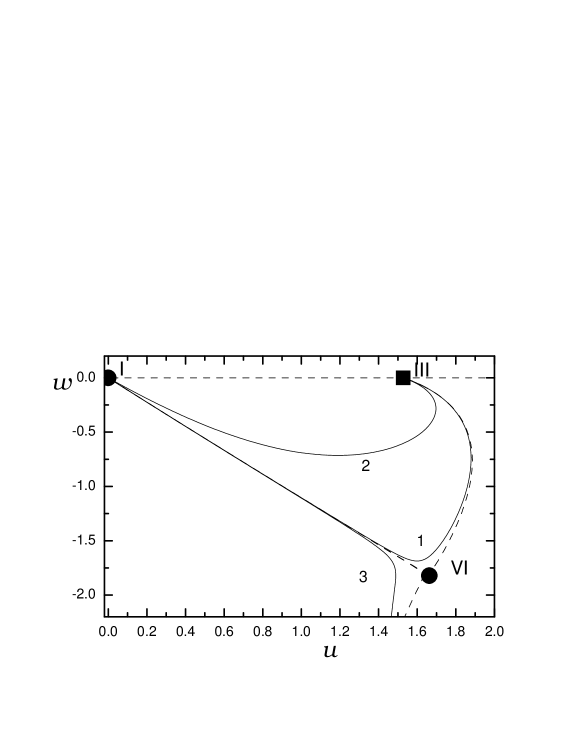
Figure 1: Flows in the space of couplings at $v=0$, $m=2$. A square denotes the stable FP, circles denote unstable FPs and dashed lines show separatrices connecting two FPs. Curves 1 and 2 correspond to a flow for the ratio $|w/u|$ chosen close above the separatrix between the FPs I and VI, while the flow 3 starts from a value $|w/u|$ below the separatrix.

Figure 2: Effective critical exponent $\gamma_{\rm eff}$ as a function of the logarithm of the flow parameter, $m=2$. Curves correspond to flows of Fig. 1 (denoted by the corresponding numbers). The dashed lines indicate the values of $\gamma$ at the corresponding FP.

In the Fig. 1 we show the flows that start from the initial values with $v=0$. All flows starting from values of couplings below the separatrix connecting FP I and VI run into the region of large negative $w$, as discussed above (e. g. flow 3 in the Fig. 1). In fact they are “runaway” solutions which may indicate the possibility of a first order transition. The curves 1 and 2 in the Fig. 1 are obtained from initial values located above the separatrix connecting FPs I and VI. We expect that these flows can not be observed for the RAM because they are far away from the condition $w/u=-m$. The flows starting above the separatrix connecting FP I with FP VI are influenced by the unstable FP VI and finally attracted by the “polymer” stable FP III. Fig. 2 shows the curves of magnetic susceptibility effective critical exponent $\gamma_{\rm eff}$ corresponding to the flows of the Fig. 1. We do not present results for other effective critical exponents, since they demonstrate qualitatively the same behaviour as $\gamma_{\rm eff}$.

Let us now consider the possible scenarios for the effective critical exponents if all initial values of couplings are non-zero. Flows starting from physical initial values for the RAM are either attracted by the stable FP we rejected as unphysical (see the last paragraph of subsection 4.2.1) or have runaway character. However the critical behaviour in the initial phase of the flow can be influenced by the physical unstable FPs. At initial values appropriate to the RAM a flow can be realized, that is affected by the unstable FP II, which describes critical behaviour of pure $m$-vector model. Thus the effective critical exponent corresponding to this flow (Fig. 3) demonstrates regions with the critical exponent of the $m$-vector model (in the given case for $m=2$). Monte Carlo calculations for $m=2$ report critical exponents similar to the pure XY model [69]. Our theory suggests that the exponents found are effective ones.

Figure 3: The effective critical exponent $\gamma_{\rm eff}$ as a function of the logarithm of the flow parameter for isotropic distribution of the local anisotropy axes, $m=2$. Dashed lines indicate the value of $\gamma$ at the corresponding FPs.

4.3.2 Cubic distribution

Flows for the cubic distribution of the random anisotropy axes have been considered already within the five-loop massive scheme [78], however the behaviour of effective critical exponents has not been studied. They confirm that the FPs of the random Ising FP XV and “polymer” FP III models are the only stable FPs. Moreover, the flows from initial conditions satisfying $u>0$, $w<0$, $u+w<0$ and $v+y>0$, $mv+y>0$ according to (21) are never attracted by the “polymer” FP III. Therefore in our investigation we restrict the initial conditions to this region. Starting with large negative $w$, the flow fast runs into the region, where the resummation method does not work. Thus the initial conditions are chosen close to the line $w/u=-m$.

Figure 4: Flows in space of couplings for $u=v=0$. The square denotes the stable FP, the circles mean unstable FPs and the dashed lines are separatrices connecting two FPs.

Figure 5: Effective critical exponent $\gamma_{\rm eff}$ as a function of the logarithm of the flow parameter. Curves correspond to flows of Fig. 4 denoted by corresponding numbers. Dashed lines indicate the value of $\gamma$ at the corresponding FPs.

As an illustration, let us first consider the trajectories with the initial conditions $u=v=0$. Solutions of the flow equations in this case are plotted in the Fig. 4. The corresponding scenarios of the behaviour of the effective critical exponent $\gamma_{\rm eff}$ are shown in the Fig. 5. The particular features of initial conditions with $u=v=0$ is, that the effective critical exponents are independent of the order parameter dimension $m$ since all $m$-dependent terms in the flow equations drop out. At large values of ratio $|w/y|$ one can observe flows which seem to be not attracted by the stable FP XV at the beginning, but finally the flows end in this FP. Therefore effective critical exponents with values overshooting the asymptotic ones can be observed (curve 1 in the Fig. 5). If flows are strongly affected by the unstable FP V, then before they crossover to asymptotic values of the dilute Ising model the critical exponents of the pure Ising model (corresponding to FP V) are observed (curve 4 in the Fig. 5). Since the effective Hamiltonian (10) with $u_{0}=v_{0}=0$ corresponds to the diluted Ising model, in Figs. 4 and 5 the picture obtained for that model [118, 126] is recovered.

Figure 6: Flows in space of couplings for $v=0$. The squares denote stable FPs, the circles mean unstable FPs and the dashed lines are separatrices connecting two FPs.

Figure 7: Effective critical exponent $\gamma_{\rm eff}$ as a function of the logarithm of the flow parameter. Curves correspond to flows of Fig. 6 denoted by corresponding numbers. Dashed lines indicate the value of $\gamma$ at the corresponding FPs.

If we “switch on” the coupling $u_{0}$ (but leave $v_{0}=0$) a richer scenario of flows is obtained. The typical ones are given in the Fig. 6. Also in this case results are independent on the order parameter dimension $m$, since all $m$-dependent terms drop out of the flow equation. The effective critical exponent $\gamma_{\rm eff}$ corresponding to these flows is shown in the next Fig. 7. There are two FPs V and X that correspond to the pure Ising model. So, there exists the possibility that flows starting from certain initial values in the space of couplings first are affected by the unstable FP V of the pure Ising model, then are attracted by the Ising FP X and only then they approach the stable FP XV. It means that within a wide range of temperature the critical exponents of pure Ising model may be observed before approaching the asymptotic regime (curve 3 in the Fig. 7). A characteristic feature of almost all flows is the non-monotonic crossover to the asymptotic values.

The effective critical behaviour, which can be observed if all initial couplings are non-zero, depends on $m$ and is described by Figs. 8, 9 and 10 for values of spin component $m=2,\,3,\,4$ correspondingly. Apart from the characteristic behaviour of effective critical exponent $\gamma_{\rm eff}$ presented by curves 1-5 of Fig. 5, a new scenarios of effective critical behaviour appear. They are presented by curves 6 and 7 in the Figs. 8-10, that demonstrate regions with effective critical exponent of the pure $m$-vector model (FP II) and the cubic model (FP VIII) correspondingly.

In connection with this result, one should mention Monte Carlo simulations of the $d=3$ RAM with cubic distribution of the random anisotropy axes [70]. For $m=2$ and weak anisotropy the results are consistent with a second order phase transition with critical exponents, which are close to those of the pure XY model. The theory shows that the asymptotic critical behaviour is governed by the random Ising critical exponent, FP XV, while critical exponents of pure model, FP II, are possible as effective ones in the certain temperature region.

Figure 8: Effective critical exponent $\gamma_{\rm eff}$ as a function of the logarithm of the flow parameter for order parameter dimension $m=2$. Dashed lines indicate the value of $\gamma$ at the corresponding FPs.

Figure 9: Effective critical exponent $\gamma_{\rm eff}$ as a function of the logarithm of the flow parameter for order parameter dimension $m=3$. Dashed lines indicate the value of $\gamma$ at the corresponding FPs.

Figure 10: Effective critical exponent $\gamma_{\rm eff}$ as a function of the logarithm of the flow parameter for order parameter dimension $m=4$. Dashed lines indicate the value of $\gamma$ at the corresponding FPs.

5 Conclusions

In the present paper we have studied the critical behaviour of three dimensional random anisotropy magnets. The experimental, numerical and theoretical investigations performed so far give contradictory results. However, two main conclusions can be drawn from the existing data. The random anisotropy with isotropic distribution of quenched anisotropy axes destroys the second order phase transition of the pure system, while for the anisotropic distribution there exists the possibility of a second order phase transition.

The standard tool for describing the critical behaviour of different systems, the field-theoretical RG, gives results in consistency with these conclusions. In particular, the absence of a stable accessible FP for an isotropic distribution of the random axes means an absence of a second order phase transition. First derived on the basis of a one-loop RG calculation [74], this conclusion found its further support in the analysis of the two- [75, 76, 77] and the five-loop [78] massive RG functions refined by resummation.

The two-loop approximation within the massive RG scheme applied to the case, when random axes are distributed along the edges of the $m$-dimensional hypercube, lead to an answer about the second order phase transition with the same set of critical exponents as those of the weakly diluted Ising systems [76, 77, 103]. This was confirmed in a recent five-loop RG calculations [78].

Although the majority of the experimental and simulation data show a effective critical behaviour, the effective critical behaviour of random anisotropy magnets was not studied extensively so far. We used the minimal subtraction scheme of the field theoretical RG approach to analyse such a behaviour. The calculations were performed within two-loop approximation combined with resummation of perturbation theory expansions. The results concerning the asymptotic critical behaviour confirm the picture obtained in the massive scheme [75, 76, 77, 103, 78].

Studying nonasymptotic critical behaviour of the $d=3$ RAM with isotropic as well as with cubic distributions of anisotropy axes we calculated the effective critical exponents. The results show that for certain initial conditions the effective critical behaviour of the random anisotropy magnets with isotropic distribution of random axes can be governed by critical exponent of the $m$-vector model at least for $m=2$ in a certain temperature interval. Also we investigated effective critical behaviour of systems described by Hamiltonian (9) with values of bare couplings differing from those of the RAM.

In the case of the RAM with cubic distribution of anisotropy axes, various scenarios of effective critical behaviour can be observed. The crossover from background behaviour described by the Gaussian critical exponents to the asymptotic random Ising behaviour demonstrates the existence of temperature regions where effective critical exponents coincide with values of the critical exponents of pure Ising, cubic and $m$-vector models. A characteristic feature of the majority of the effective critical exponent is the appearance of peaks before the crossover to the asymptotic limit.

In conclusion, we want to attract attention to the importance of determining the nonasymptotic critical regime in the investigation of the critical behaviour of random anisotropy magnets. As our investigation shows being not close enough to the asymptotic critical regime different values of critical exponents can be obtained, they have been shown to be effective ones.

This work was supported by the Fonds zur Förderung der wissenschaftlichen Forschung under Project No. 16574-PHY. Yu. H. and M. D. acknowledge French-Ukrainian cooperation Dnipro project and useful comments of Bertrand Berche and Taras Yavors’kii.

Appendix A Appendix

Here, we describe the procedure of the RAM representation in terms of the functional integrals. The case of weak anisotropy is of special interest and to introduce the controlling parameter $D/\bar{J}$ an appropriate normalization of spins can be used $\vec{S}^{\prime}=\vec{S}\sqrt{\bar{J}}$. Then, Hamiltonian (1) is rewritten in form:

$${\mathcal{H}}=-\sum_{{\bf R},{\bf R^{\prime}}}\frac{J_{{\bf R},{\bf R^{\prime}}}}{\bar{J}}\vec{S^{\prime}}_{\bf R}\vec{S^{\prime}}_{\bf R^{\prime}}-\frac{D}{\bar{J}}\sum_{{\bf R}}(\hat{x}_{\bf R}\vec{S^{\prime}}_{\bf R})^{2}.$$ (56)

It is useful to perform a Fourier transformation for the interaction part of (2) and leave the random axis part as it is, after that the Hamiltonian reads:

$${\mathcal{H}}=-\sum_{k}\nu(k)\vec{S^{\prime}}_{\bf k}\vec{S^{\prime}}_{\bf-k}-D^{\prime}\sum_{R}(\hat{x}_{\bf R}\vec{S^{\prime}}_{\bf R})^{2},$$ (57)

where $\vec{S^{\prime}}_{\bf k}$ and $\nu(k)$ are Fourier transforms of spin and interaction correspondingly, $D^{\prime}=D/\bar{J}$.

For the fixed configuration of the local random anisotropy axes $\{\hat{x}_{\bf R}\}$ the configuration-dependent partition function is written

$$Z(\{\hat{x}_{\bf R}\})={\rm Sp}\,\,e^{-{\beta\mathcal{H}}},$$ (58)

where the Hamiltonian $\mathcal{H}$ is given by (57), $\beta$ is the inverse temperature and the trace means integration over the surface of $m$-dimensional hypersphere with unit radius: ${\rm Sp}(\dots)=\int d\vec{S^{\prime}}_{\bf R}(\dots)\delta(|\vec{S^{\prime}}_{\bf R}|-1)$.

To avoid taking trace of products of spins one can apply the Stratonovich-Hubbard transformation to expression (58) and arrive at the following form of the partition function:

$$Z(\{\hat{x}_{\bf R}\}) \sim {\rm Sp}\int(d\vec{\phi})\exp\Big{\{}-\frac{1}{4}\sum_{k}\frac{1}{\beta\nu(k)}|\vec{\phi}_{\bf k}|^{2}+$$ (59)

$$\sum_{R}\vec{S^{\prime}}_{\bf R}\vec{\phi}_{\bf R}+\beta D^{\prime}\sum_{R}(\hat{x}_{\bf R}\vec{S^{\prime}}_{\bf R})^{2}\Big{\}},$$

where $\vec{\phi}_{\bf k}$ is the Fourier transform of the $m$-component field variable $\vec{\phi}_{\bf R}$, introduced by the Stratonovich-Hubbard transformation. The integral in (59) means a functional integration in the space of the field variables $\vec{\phi}$. Here, we omit the normalization coefficient before the integral since it does not alter the behaviour of system near critical point.

Now the trace operation for the spins concerns only the last two terms of the exponent in (59). Expanding the exponential function in a Taylor series, performing the integration with use of generalized $m$-dimensional spherical coordinates and finally reexponentiating the obtained series, one gets:

$$Z(\{\hat{x}_{\bf R}\}) \sim \int(d\vec{\phi})\exp\Big{\{}{-}\frac{1}{4}\sum_{k}\frac{|\vec{\phi}_{\bf k}|^{2}}{\beta\nu(k)}{+}\frac{\sum_{\bf R}|\vec{\phi}_{\bf R}|^{2}}{2m}\left(1-\frac{2\beta D^{\prime}}{m(m+2)}\right){-}$$ (60)

$$\frac{\sum_{\bf R}|\vec{\phi}_{\bf R}|^{4}(m+4+\beta D^{\prime}(m+6))}{4m^{2}(m+2)(m+4)}{+}\frac{\beta D^{\prime}}{m(m+2)}\sum_{\bf R}\left(\vec{\phi}_{\bf R}\hat{x}_{\bf R}\right)^{2}{-}$$

$$\frac{2\beta D^{\prime}\sum_{\bf R}|\vec{\phi}_{\bf R}|^{2}\left(\vec{\phi}_{\bf R}\hat{x}_{\bf R}\right)^{2}}{m^{2}(m+2)(m+4)}+\dots\Big{\}},$$

Here, we omit all terms independent on $\phi$ since they give only a shift of the free energy. Expression (60) has been obtained under assumption of a weak anisotropy $D^{\prime}<<1$, thus the only terms in first order in $D^{\prime}$ were taken into account. Furthermore, there is no interest in terms of order higher then fourth order in $\phi$, since they are irrelevant in the RG calculations of the critical properties of the model. They may be relevant when multicritical behaviour is studied.

Since the small wave lengths are relevant for the critical behaviour, it is possible to use the expansion of the interaction Fourier image at small $\bf k$: ${(\beta\nu(k))}^{-1}=c_{0}+b_{0}{\bf k}^{2}+\dots$. Then transforming back to real space and passing to the continuous limit by replacing summation over $\bf R$ by the familiar $d$-dimensional integral one obtains:

$$Z(\{\hat{x}_{\bf R}\}\sim\int(d\vec{\phi})e^{{\mathcal{H}}(\hat{x}_{\bf R},\vec{\phi}_{\bf R})},$$ (61)

where

$${\mathcal{H}}({\hat{x}_{\bf R},\vec{\phi}_{\bf R}}) = -\int d^{d}R\Big{\{}\frac{1}{2}\left[r_{0}|\vec{\phi}_{\bf R}|^{2}+\left|\vec{\nabla}\vec{\phi}_{\bf R}\right|^{2}\right]{-}D_{1}\left(\vec{\phi}_{\bf R}\hat{x}_{\bf R}\right)^{2}{+}v_{1}|\vec{\phi}_{\bf R}|^{4}+$$ (62)

$$z|\vec{\phi}_{\bf R}|^{2}\left(\vec{\phi}_{\bf R}\hat{x}_{\bf R}\right)^{2}+\dots\Big{\}}.$$

Here, the field $\phi$ was normalized to get coefficient for gradient term equal to unity and $r_{0}=\frac{1{}}{b_{0}}\left(c_{0}-\frac{2}{m}(1-\frac{2\beta D^{\prime}}{m(m+2)})\right)$, $v_{1}=\frac{(m+4+\beta D^{\prime}(m+6))}{{b_{0}}^{2}m^{2}(m+2)(m+4)}$, $D_{1}=\frac{4\beta D^{\prime}}{{b_{0}}^{2}m(m+2)}$, $z=\frac{8\beta D^{\prime}}{{b_{0}}^{2}m^{2}(m+2)(m+4)}$.

References

- [1]
- [2] For a recent reviews on some related topics see e.g.: Yu. Holovatch (Ed.), Order, Disorder and Criticality. Advanced Problems of Phase Transition Theory, World Scientific, Singapore, 2004.
- [3] A. Pelissetto, E. Vicari, Phys. Rep. 368 (2002) 549.
- [4] R. Folk, Yu. Holovatch, T. Yavors’kii, Physics-Uspekhi 46 (2003) 169 [Uspekhi Fizicheskikh Nauk 173 (2003) 175]; preprint cond-mat/0106468.
- [5] D. P. Belanger, A. P. Young, J. Magn. Magn. Mater. 100 (1991) 272.
- [6] R. W. Cochrane, R. Harris, M. J. Zuckermann, Phys. Reports 48 (1978) 1.
- [7] E. Brézin, J. C. Le Guillou, J. Zinn-Justin, in: C. Domb, M. S. Green (Eds.), Phase Transitions and Critical Phenomena, Vol. 6, Academic Press, London, 1976, p. 127; D. J. Amit, Field Theory, the Renormalization Group, and Critical Phenomena, World Scientific, Singapore, 1989; J. Zinn-Justin, Quantum Field Theory and Critical Phenomena, Oxford University Press, 1996; H. Kleinert, V. Schulte-Frohlinde, Critical Properties of -Theories, World Scientific, Singapore, 2001.
- [8] R. Harris, M. Plischke, M. J. Zuckermann, Phys. Rev. Lett. 31 (1973) 160.
- [9] J. M. D. Coey, T. R. McGuire, B. Tissier, Phys. Rev. B 24 (1981) 1261.
- [10] S. von Moral, B. Barbara, T. R. McGuire, R. Gambino, J. Appl. Phys. 53 (1982) 2350 ; S. von Moral, T. R. McGuire, R. Gambino, B. Barbara, J. Appl. Phys. 53 (1982) 7666.
- [11] B. Barbara, B. Dieny, A. Lienard, J. R. Rebouillat, B. Boucher, J. Schweizer, Solid State Commun. 55 (1985) 463 .
- [12] B. Dieny, B. Barbara, Phys. Rev. Lett. 57 (1986) 1169.
- [13] K. M. Lee, M. J. O’Shea, Phys. Rev. B 48 (1993) 13614.
- [14] J. Benejelloun, M. Baran, H. Lassri, O. Oukris, R. Krishnan, M.Omri, M.Ayadi, J. Magn. Magn. Mater. 204 (1999) 68.
- [15] N. Hassanain, A. Berrada, H. Lassri, R. Krishnan, J. Magn. Magn. Mater. 140-144 (1995) 337.
- [16] B. Dieny, B. Barbara, J. Phys. (Paris) 46 (1985) 293.
- [17] B. Barbara, B. Dieny, Physica B 130 (1985) 245.
- [18] B. Barbara, M. Couach, B. Dieny, Europhys. Lett. 3 (1987) 1129.
- [19] M. J. O’Shea, K. M. Lee, F. Othman, Phys. Rev. B 34 (1986) 4944.
- [20] G. R. Gruzalski, D. J. Sellmyer, Phys. Rev. B 20 (1979) 194.
- [21] A. del Moral, J. I. Arnaudas, K. A. Mohammed, Solid State Commun. 58 (1986) 395.
- [22] D. J. Sellmyer, S. Nafis, Phys. Rev. Lett. 57 (1986) 1173.
- [23] A. del Moral, J. I. Arnaudas, Phys. Rev. B 39 (1989) 9453.
- [24] R. I. Bewley, R. Ciwinski, J. Magn. Magn. Mater. 140-144 (1995) 869.
- [25] C. de la Fuente, J. I. Arnaudas, A. del Moral, M. Ciria, J. Magn. Magn. Mater. 157/158 (1996) 535.
- [26] M. J. O’Shea, S. G. Cornelison, Z. D. Chen, D. J. Sellmyer, Solid State Commun. 46 (1983) 313.
- [27] S. G. Cornelison, D. J. Sellmyer, Phys. Rev. B 30 (1984) 2845.
- [28] J. Tejada, B. Martinez, A. Labarta, R. Größinger, H. Sassik, M. Vazquez, A. Hernando, Phys. Rev. B 42 (1990) 898.
- [29] L. Driouch, R Krishnan, J. Voiron, J. Magn. Magn. Mater. 157/158 (1996) 149.
- [30] M. Slimani, M. Hamdoun, M. Tlemçani, H. Arhchouri, S. Sayouri, Physica B 240 (1997) 372.
- [31] D. J. Sellmyer, S. Nafis, J. Appl. Phys. 57 (1985) 3584.
- [32] R. Krishnan, H. Lassri, L. Driouch, J. Magn. Magn. Mater. 140-144 (1995) 355.
- [33] R. Krishnan, L. Driouch, H. Lassri, Y. Dumond, A. Ajan, S. N. Shringi, S. Prasad, J. Magn. Magn. Mater. 163 (1996) 353.
- [34] A. Itri, H. Lassri, M. E. Yamani, Physica B 269 (1999) 189.
- [35] G. T. Bhandage, A. Belayachi, M. Noguès, G. Villers, J. L. Dormann, H. V. Keer, J. Magn. Magn. Mater. 166 (1997) 141.
- [36] H. Kato, N. Kurita, Y. Ando, T. Miyazaki, M. Motokawa, J. Magn. Magn. Mater. 189 (1998) 263.
- [37] P. M. Gehring, M. B. Salamon, A. del Moral, J. I. Arnaudas, Phys. Rev. B 41 (1990) 9134.
- [38] E. Joven, A. del Moral, J. I. Arnaudas, J. Appl. Phys. 69 (1991) 5069.
- [39] A. del Moral, J. I. Arnaudas, C. de la Fuente, M. Ciria, E. Joven, P. M. Gehring J. Appl. Phys. 76 (1994) 6180.
- [40] A. del Moral, J. I. Arnaudas, P. M. Gehring J. Phys. 6 (1994) 4779.
- [41] M. Ciria, A. del Moral, J. I. Arnaudas, J. S. Abell, Y. J. Bi, J. Magn. Magn. Mater. 140-144 (1995) 1115.
- [42] A. del Moral, C. de la Fuente, J. I. Arnaudas, Phys. Rev. B 54 (1996) 12245.
- [43] A. del Moral, C. de la Fuente, J. I. Arnaudas, J. Phys. 8 (1996) 6945.
- [44] Y. Homma, Y. Takakuwa, Y. Shiokawa, K. Suzuki, J. Alloys and Compounds 275-277 (1998) 459.
- [45] Y. Homma, Y. Takakuwa, Y. Shiokawa, D.X. Li, K. Sumiyama, K. Suzuki, J. Alloys and Compounds 275-277 (1998) 665.
- [46] S. Itoh, Y. Homma, Y. Shiokawa, M. Akabori, A. Itoh, Physica B 281&282 (2000) 230.
- [47] D. R. Taylor, W. J. L. Buyers, Phys. Rev. B 54 (1996) R3734.
- [48] D. R. Taylor, I. P. Swainson, J. Magn. Magn. Mater. 226-230, (2001) 1338.
- [49] P. Zhou, B. G. Morin, J. S. Miller, A. J. Epstein, Phys. Rev. B 48 (1993) 1325; M. A. Gîrţu, C. M. Wynn, J. Zhang, J. S. Miller, A. J. Epstein, Phys. Rev. B 61 (2000) 492.
- [50] A. Hernando, M. Vázquez, T. Kulik, C. Prados, Phys. Rev. B 51 (1995) 3581; G. Herzer, J. Magn. Magn. Mater. 157/158 (1996) 133.
- [51] W. C. Nunes, M. A. Novak, M. Knobel, A. Hernando, J. Magn. Magn. Mater. 226-230 (2001) 1856.
- [52] D.J. Sellmyer, M. J. O’Shea, in: D. H. Ryan (Ed.), Recent progress in random magnets, World Scientific, Singapore, 1992, p. 71.
- [53] A. Aharony, E. Pytte, Phys. Rev. Lett 45 (1980) 1583.
- [54] For review see E. M. Chudnovsky, in: J. A. Fernandez-Baca, W.-Y. Ching (Eds.), The Magnetism of Amorphous Metals and Alloys, World Scientific, Singapore, 1992, p. 143.
- [55] M. Fähnle, W.-U. Kellner, H. Kronmüller, Phys. Rev. B 35 (1987) 3640.
- [56] M. C. Chi, R. Alben, J. Appl. Phys. 48 (1977) 2987.
- [57] R. Harris, S. H. Sung, J. Phys. F 8 (1978) L299.
- [58] M. C. Chi, T. Egami, J. Appl. Phys. 50 (1979) 1651.
- [59] R. Harris, J. Phys. F 10 (1980) 2545.
- [60] C. Jayaprakash, S. Kirkpatrick, Phys. Rev B 21 (1980) 4072.
- [61] A. Chakrabarti, Phys. Rev. B 36 (1987) 5747.
- [62] R. Fisch, Phys. Rev. B 39 (1989) 873.
- [63] R. Fisch, Phys. Rev. B 42 (1990) 540.
- [64] R. Fisch, Phys. Rev. Lett. 66 (1991) 2041.
- [65] P. Reed, J. Phys. C 24 (1991) L117.
- [66] R. Fisch, Phys. Rev. B 58 (1998) 5684.
- [67] M. Itakura, Phys. Rev. B 68 100405 (2003); e-print: cond-mat/0303552
- [68] R. Fisch, Phys. Rev. B 62 (2000) 361.
- [69] U. K. Rößler, Phys. Rev. B 59 (1999) 13577.
- [70] R. Fisch, Phys. Rev. B 48 (1993) 15764.
- [71] E. Callen, Y. J. Liu, J. R. Cullen, Phys. Rev. B 16 (1979) 263; J. D. Patterson, G. R. Gruzalski, D. J. Sellmyer, Phys. Rev. B 18 (1978) 1377.
- [72] R. Harris, D. Zobin, J. Phys. F 7 (1977) 337.
- [73] B. Derrida and J. Vannimenus, J. Phys. C 13 (1980) 3261.
- [74] A. Aharony, Phys. Rev. B 12 (1975) 1038.
- [75] M. Dudka, R. Folk, Yu. Holovatch, Condens. Matter Phys. 4 (2001) 77.
- [76] M. Dudka, Yu. Holovatch, R. Folk, in: W. Janke, A. Pelster, H.-J. Schmidt and M. Bachmann (Eds)., Fluctuating Paths and Fields, Singapore, World Scientific, 2001, p. 457.
- [77] Yu. Holovatch, V. Blavats’ka, M. Dudka, C. von Ferber, R. Folk, T. Yavors’kii, Int. J. Mod. Phys. B. 16 (2002) 4027.
- [78] P. Calabrese, A. Pelissetto, E. Vicari, cond-mat/0311576
- [79] J.-H. Chen, T. C. Lubensky, Phys. Rev. B 16 (1977) 2106.
- [80] Y. Imry, S.-k. Ma, Phys. Rev. Lett 35 (1975) 1399.
- [81] R. Alben, J. J. Becker, and M. C. Chi, J. Appl. Phys. 49 (1978) 1653.
- [82] R.A. Pelcovits, E. Pytte, J. Rudnick, Phys. Rev. Lett. 40 (1978) 476.
- [83] R. A. Pelcovits, E. Pytte, J. Rudnick, Phys. Rev. Lett. 48 (1982) 1297.
- [84] V. J. Emery, Phys. Rev. B 11 (1975) 239.
- [85] R. A. Pelcovits, Phys. Rev. B 19 (1979) 465.
- [86] A. Aharony, E. Pytte, Phys. Rev. B 27 (1983) 5872.
- [87] Y. Y. Goldschmidt, Nucl. Phys. B225, [F59] (1983) 123.
- [88] J. Villian, J. F. Fernandez, Z. Phys. B 54 (1984) 139.
- [89] V. S. Dotsenko, M. V. Fiegelman, J. Phys. C 16 (1983) L803.
- [90] D. E. Feldman, JETP Lett. 70 (1999) 135.
- [91] D. E. Feldman, Phys. Rev. B 61 (2000) 382.
- [92] A. M. Khorunzhy, B. A. Khorunzhenko, L. A. Pastur, M. V. Shcherbina, in: C. Domb, J. L. Lebowitz (Eds.), Phase Transitions and Critical Phenomena, Vol. 15, Academic Press, London, 1992, p.74.
- [93] A. Khurana, A. Jagannathan, M. J. Kosterlitz, Nucl. Phys. B240, [F312] (1984) 1.
- [94] Y. Y. Goldschmidt, Phys. Rev. B 30 (1984) 1632.
- [95] A. Jagannathan, B. Schaub, M. J. Kosterlitz, Nucl. Phys. B265 [F515] (1986) 324.
- [96] D. S. Fisher, Physica A 177 (1991) 84.
- [97] E. F. Shender, J. Phys. C 13 (1980) L339.
- [98] R. Fisch, A. B. Harris, Phys. Rev. B 41 (1990) 11305.
- [99] A. B. Harris, R. G. Caflisch, J. R. Banavar, Phys. Rev. B 35 (1987) 4929.
- [100] K. H. Fischer, A. Zippelius, J. Phys. C 18 (1985) L1139.
- [101] D. Mukamel, G. Grinstein, Phys. Rev. B 25 (1982) 381.
- [102] A. L. Korzhenevskii and A. A. Luzhkov, Zh. Eksp. Teor. Fiz. 94 (1988) 250 [Sov. Phys. JETP 67 (1988) 1229].
- [103] M. Dudka, R. Folk, Yu. Holovatch, Condens. Matter Phys. 4 (2001) 459.
- [104] A. J. Bray, M. A. Moore, J. Phys. C 18 (1985) L139.
- [105] A. Chakrabarti, Phys. Rev. B 39 (1989) 2807; P. Reed, J. Phys. A 24 (1991) L1299; D. R. Denholm, T. J. Sluckin, Phys. Rev. B 48 (1993) 901.
- [106] D. E. Feldman, Phys. Rev. B 56 (1997) 3167.
- [107] H. Thomas, in: T. Riste (Ed.), Ordering in Strongly-Flucktuating Condensed Matter Systems, Plenum, New York, 1980, p. 453.
- [108] R. A. Serota, P. A. Lee, Phys. Rev B 34 (1986) 1806.
- [109] R. Dickman, E. M. Chudnovski, Phys. Rev B 44 (1991) 4397.
- [110] P. Reed, J. Phys. A 26 (1993) L807.
- [111] R. Brout, Phys. Rev. 115 (1959) 824.
- [112] An extended analysis of the RAM effective critical behavior may be found in: M. Dudka, Ph.D. Thesis, ICMP, Lviv, 2003.
- [113] G. ’t Hooft, M. Veltman, Nucl. Phys. B 44 (1972) 189; G. ’t Hooft, Nucl. Phys. B 61 (1973) 455. In the minimal subtraction scheme only pole terms appearing in vertex functions are subtracted. It is used together with dimensional regularization.
- [114] K. Wilson, M. E. Fisher, Phys. Rev. Lett. 28 (1972) 240.
- [115] R. Schloms and V. Dohm, Europhys. Lett. 3 (1987) 413; R. Schloms and V. Dohm, Nucl. Phys. B 328 (1989) 639.
- [116] G. Grinstein, A. Luther, Phys. Rev. B 13 (1976) 1329.
- [117] D. E. Khmel’nitskii, Zh. Eksp. Teor. Fiz. 68 (1975) 1960 [ Sov. Phys. JETP 41 (1975) 981]; A. B. Harris, T. C. Lubensky, Phys. Rev. Lett. 33 (1974) 1540; T. C. Lubensky, Phys. Rev. B 11 (1975) 3573.
- [118] R. Folk, Yu. Holovatch, T. Yavors’kii, Phys. Rev. B 61 (2000) 15114.
- [119] G. A. Baker, Jr., B. G. Nickel, D. I. Meiron, Phys. Rev. B 17, (1978) 1365.
- [120] P. J. S. Watson, J. Phys. A 7 (1974) L167.
- [121] G. A. Baker, Jr., P. Graves-Morris, Padé Approximants (Addison-Wesley: Reading, MA, 1981)
- [122] Note that the resummation is performed for the polynomial for the inverse exponent.
- [123] P. Calabrese, A. Pelissetto, E. Vicari, Phys. Rev. B 67 (2003) 024418; e-print:cond-mat/0202292
- [124] N. A. Shpot, On the critical behaviour of three-dimensional cubic crystals with random impurities, Prepr. ITF-89-21P, Kiev, 1989.
- [125] A. Pelissetto, E. Vicari, Phys.Rev. B 62 (2000) 6393.
- [126] P. Calabrese, P. Parruccini, A. Pelissetto, E. Vicari, Phys. Rev. E 69 (2004) 036120; e-print: cond-mat/0307699
- [127] P. Calabrese, V. Martín-Mayor, A. Pelissetto, E. Vicari, Phys. Rev. E 68 (2003) 036136.
- [128] J. S. Kouvel, M. E. Fisher, Phys. Rev. 136 (1964) A1626; E. K. Riedel, F. J. Wegner, Phys. Rev. B 9 (1974) 294.
- [129] This approximation has also been used in the earlier work on diluted models H. K. Janssen, K. Oerding, E. Sengespeick, J. Phys. A 28 (1995) 6073; R. Folk, Yu. Holovatch, T. Yavors’kii, Phys. Rev. B 61 (2000) 15114; and in other cases E. Frey, F. Schwabl, Phys. Rev. B 42 (1990) 8261; I. Nasser, R. Folk, Phys. Rev. B 52 (1995) 15799.
- [130] M. Dudka, Yu. Holovatch, R. Folk, D. Ivaneiko, J. Magn. Magn. Mater. 256 (2003) 243.