Shot noise in resonant tunneling through an interacting quantum dot with intradot spin-flip scattering

Abstract

In this paper, we present theoretical investigation of the zero-frequency shot noise spectra in electron tunneling through an interacting quantum dot connected to two ferromagnetic leads with possibility of spin-flip scattering between the two spin states by means of the recently developed bias-voltage and temperature dependent quantum rate equations. For this purpose, a generalization of the traditional generation-recombination approach is made for properly taking into account the coherent superposition of electronic states, i.e., the nondiagonal density matrix elements. Our numerical calculations find that the Fano factor increases with increasing the polarization of the two leads, but decreases with increasing the intradot spin-flip scattering.

I INTRODUCTION

Recent rapid development of spintronic and single electron devices has resulted in intensive studies of spin-related phenomena in various resonant tunneling structures.Prinz ; Wolf One of the devices of interest is a quantum dot (QD), sandwiched between two ferromagnetic electrodes.dot1 ; dot2 ; dot3 This kind of spin-related single-electron devices suffers inevitably intrinsic relaxations (decoherence) due to the spin-orbital interactionFedichkin or the hyperfine-mediated spin-flip transition.Erlingsson The effect of the intrinsic decoherence on the quantum transport properties in these devices still deserves more investigation. As is well known, measurement of shot noise, which is a consequence of the discrete nature of the electric charge, can provide information about the microscopic interactions and the statistics of particles, which is not available through the conductance measurement alone.Beenakker ; Blanter Therefore, it is remarkably desirable to expand our knowledge about the shot noise spectra in such a spin-related single-electron tunneling device.

For metallic QD without intrinsic decoherence, the zero-frequency Fano factor, which quantifies correlations with respect to the uncorrelated Poissonian noise, was analyzed with the classical rate equation approach (classical shot noise) in Refs.[Hershfield, ; Korotkov, ; Hanke, ]. However, in order to account for the quantum effects during sequential tunneling processes, such as coherence and superposition of the wave functions and various intrinsic interactions, a more elaborate quantum description is required. The quantum rate equation approach is a suitable tool for accomplishing this task.Nazarov ; Gurvitz ; Fedichkin ; Dong In particular, some of the authors, Dong, Cui, and Lei, recently established the quantum rate equations for coherent tunneling through the coupled quantum systems with a bias-voltage and temperature dependent version.Dong Consequently, these equations allow us to study the quantum tunneling in moderately small bias-voltage region, where the quantum coherence plays more prominent role. Therefore, the purpose of the present paper is to develop an approach for calculation of the coherent effect, due to the intrinsic spin scattering, on the zero-frequency shot noise spectra in an interacting QD weakly connected with two ferromagnetic leads based on the quantum rate equations.

The rest of this paper is organized as follows. In section II, we introduce the Hamiltonian for the interacting QD with intradot spin scattering, and then give the quantum rate equations. In section III, we describe our methodology for evaluating the quantum shot noise. In section IV, we present the numerical results and discussions. Finally, a brief summary is presented in section V.

II SINGLE QUANTUM DOT: Model and quantum rate equations

The system that we study is a single QD with an arbitrary intradot Coulomb interaction $U$ connected with two ferromagnetic leads. In this paper, we assume that the tunneling coupling between the dot and the leads is weak enough to guarantee no Kondo effect and that the QD is in the Coulomb blockade regime. For simplicity, we model the intrinsic spin relaxation with a phenomenological spin-flip term $R$ and assume that this spin-flip process just happen in the dot (the spin conserving tunneling).

Moreover, we assume that the temperature is small enough to see the effects due to the discrete charging and discrete structure of the energy levels, i.e. $k_{B}T\ll U$,$\Delta$, where, $\Delta$ is the energy spacing between orbital levels. Each of the two leads is separately in thermal equilibrium with the chemical potential $\mu_{\eta}$, which is assumed to be zero in the equilibrium condition and is taken as the energy reference throughout the paper. In the nonequilibrium case, the chemical potentials of the leads differ by the applied bias $V$. We are interested in the regime $eV\ll\Delta$, where only one dot level $(\epsilon_{d})$ contributes to the transport. Here we neglect Zeeman splitting of the level due to weak magnetic fields $B$ ($g\mu_{B}B<k_{B}T)$, which means that both the spin-up and spin-down transports through the dot go through the same orbital level $\epsilon_{d}$. Therefore, the Hamiltonian of resonant tunneling through a single QD can be written as:Dong

$$H = \sum_{\eta,k,\sigma}\epsilon_{\eta k\sigma}c_{\eta k\sigma}^{\dagger}c_{\eta k\sigma}^{{\phantom{\dagger}}}+\epsilon_{d}\sum_{\sigma}c_{d\sigma}^{\dagger}c_{d\sigma}^{{\phantom{\dagger}}}+R(c_{d\uparrow}^{\dagger}c_{d\downarrow}^{{\phantom{\dagger}}}$$ (2)

$$+c_{d\downarrow}^{\dagger}c_{d\uparrow}^{{\phantom{\dagger}}})+Un_{d\uparrow}n_{d\downarrow}+\sum_{\eta,k,\sigma}(V_{\eta\sigma}c_{\eta k\sigma}^{\dagger}c_{d\sigma}^{{\phantom{\dagger}}}+{\rm{H.c.}}),$$

where $c_{\eta k\sigma}^{\dagger}$ ($c_{\eta k\sigma}$) and $c_{d\sigma}^{\dagger}$ ($c_{d\sigma}$) are the creation (annihilation) operators for electrons with momentum $k$, spin-$\sigma$ and energy $\epsilon_{\eta k\sigma}$ in the lead $\eta$ ($={\rm L,R}$) and for a spin-$\sigma$ electron on the QD, respectively. $n_{d\sigma}=c_{d\sigma}^{\dagger}c_{d\sigma}^{{\phantom{\dagger}}}$ is the occupation operator in the QD. The fourth term describes the Coulomb interaction among electrons on the QD. The fifth term represents the tunneling coupling between the QD and the reservoirs. We assume that the coupling strength $V_{\eta\sigma}$ is spin-dependent being capable of describing the ferromagnetic leads.

Under the assumption of weak coupling between the QD and the leads, and applying the wide band limit in the two leads, electronic transport through this system in sequential regime can be described by the bias-voltage and temperature dependent quantum rate equations for the dynamical evolution of the density matrix elements:Dong

$$\dot{\rho}_{00}=\sum_{\eta\sigma}(\Gamma_{\eta\sigma}^{-}\rho_{\sigma\sigma}-\Gamma_{\eta\sigma}^{+}\rho_{00}),$$ (4a)

$$\dot{\rho}_{\sigma\sigma} = \sum_{\eta}\Gamma_{\eta\sigma}^{+}\rho_{00}+\sum_{\eta}\widetilde{\Gamma}_{\eta\bar{\sigma}}^{-}\rho_{dd}-\sum_{\eta}(\Gamma_{\eta\sigma}^{-}+\widetilde{\Gamma}_{\eta\bar{\sigma}}^{+})\rho_{\sigma\sigma}$$ (4b)

$$+iR(\rho_{\sigma\bar{\sigma}}-\rho_{\bar{\sigma}\sigma}),$$

$$\dot{\rho}_{\sigma\bar{\sigma}}=iR(\rho_{\sigma\sigma}-\rho_{\bar{\sigma}\bar{\sigma}})-\frac{1}{2}\sum_{\eta}(\widetilde{\Gamma}_{\eta\sigma}^{+}+\widetilde{\Gamma}_{\eta\bar{\sigma}}^{+}+\Gamma_{\eta\sigma}^{-}+\Gamma_{\eta\bar{\sigma}}^{-})\rho_{\sigma\bar{\sigma}},$$ (4c)

$$\dot{\rho}_{dd}=\sum_{\eta}\widetilde{\Gamma}_{\eta\downarrow}^{+}\rho_{\uparrow\uparrow}+\sum_{\eta}\widetilde{\Gamma}_{\eta\uparrow}^{+}\rho_{\downarrow\downarrow}-\sum_{\eta}(\widetilde{\Gamma}_{\eta\uparrow}^{-}+\widetilde{\Gamma}_{\eta\downarrow}^{-})\rho_{dd},$$ (4d)

($\sigma=\uparrow,\downarrow$ stands for electron spin and $\bar{\sigma}$ is the spin opposite to $\sigma$). The statistical expectations of the diagonal elements of the density matrix, $\rho_{ii}$ ($i=\{0,\sigma,d\}$), give the occupation probabilities of the resonant level in the QD as follows: $\rho_{00}$ denotes the occupation probability that central region is empty, $\rho_{\sigma\sigma}$ means that the QD is singly occupied by a spin-$\sigma$ electron, and $\rho_{dd}$ stands for the double occupation by two electrons with different spins. Note that they must satisfy the normalization relation $\rho_{00}+\rho_{dd}+\sum_{\sigma}\rho_{\sigma\sigma}=1$. The non-diagonal elements $\rho_{\sigma\bar{\sigma}}$ describe the coherent superposition of different spin states. These temperature-dependent tunneling rates are defined as $\Gamma_{\eta\sigma}^{\pm}=\Gamma_{\eta\sigma}f_{\eta}^{\pm}(\epsilon_{d})$ and $\widetilde{\Gamma}_{\eta\sigma}^{\pm}=\Gamma_{\eta\sigma}f_{\eta}^{\pm}(\epsilon_{d}+U)$, where $\Gamma_{\eta\sigma}$ are the tunneling constants, $f_{\eta}^{+}(\omega)=\{1+e^{(\omega-\mu_{\eta})/T}\}^{-1}$ is the Fermi distribution function of the $\eta$ lead and $f_{\eta}^{-}(\omega)=1-f_{\eta}^{+}(\omega)$. Here, $\Gamma_{\eta\sigma}^{+}$ ($\Gamma_{\eta\sigma}^{-}$) describes the tunneling rate of electrons with spin-$\sigma$ into (out of) the QD from (into) the $\eta$ lead without the occupation of the $\bar{\sigma}$ state. Similarly, $\widetilde{\Gamma}_{\eta\sigma}^{+}$ ($\widetilde{\Gamma}_{\eta\sigma}^{-}$) describes the tunneling rate of electrons with spin-$\sigma$ into (out of) the QD, when the QD is already occupied by an electron with spin-$\bar{\sigma}$, revealing the modification of the corresponding rates due to the Coulomb repulsion. The particle current $I_{\eta}$ flowing from the lead $\eta$ to the QD is

$$I_{\eta}/e=\sum_{\sigma}(\widetilde{\Gamma}_{\eta\sigma}^{-}\rho_{dd}+\Gamma_{\eta\sigma}^{-}\rho_{\sigma\sigma}-\widetilde{\Gamma}_{\eta\bar{\sigma}}^{+}\rho_{\sigma\sigma}-\Gamma_{\eta\sigma}^{+}\rho_{00}).$$ (5)

This formula demonstrates that the current is totally determined by the diagonal elements of the density matrix of the central region. However, the nondiagonal element of the density matrix is coupled with the diagonal elements in the rate equation (4b), and therefore indirectly influences the tunneling current.

III Quantum shot noise formula

There is a well-established procedure, namely, the generation-recombination approach for multielectron channels, for the calculation of the noise power spectrum based on the classical rate equations (classical shot noise).Hershfield ; Korotkov ; Hanke In this section we modify this approach in order to take into account the nondiagonal density matrix elements and derive the general expression for a quantum shot noise for the single QD.

Before proceeding with investigation of current correlation, it is helpful to rewrite the quantum rate equations as matrix form:

$$\frac{d{\bm{\rho}}(t)}{dt}=\mathbf{M}\ {\bm{\rho}}(t)\ ,$$ (6)

where ${\bm{\rho}}(t)=(\rho_{00},\rho_{\uparrow\uparrow},\rho_{\downarrow\downarrow},\rho_{dd},\rho_{\uparrow\downarrow},\rho_{\downarrow\uparrow})^{T}$ is a vector whose components are the density matrix elements, and the $6\times 6$ matrix ${\bf M}$ can be easily obtained from Eqs. (4). Correspondingly, we can write the average electrical currents across the left ($I_{L}$) and right ($I_{R}$) junctions at time $t$ as:

$$\langle I_{L(R)}(t)\rangle=-e\sum_{k}\left[\hat{\Gamma}_{L(R)}{\bm{\rho}}(t)\right]_{k},$$ (7)

where $\hat{\Gamma}_{L}$ and $\hat{\Gamma}_{R}$ are current operators and the summation goes over all vector $[\hat{\Gamma}_{L(R)}{\bm{\rho}}(t)]$ elements ($k=1,2,\cdots,6$). The current operators contain the rates for tunneling across the left and right junctions respectively,Hershfield and they can be read from Eq. (5) as:

$$\hat{\Gamma}_{\eta}=\pm\left(\begin{array}[]{cccccc}0&\Gamma_{\eta\uparrow}^{-}&\Gamma_{\eta\downarrow}^{-}&0&0&0\\ -\Gamma_{\eta\uparrow}^{+}&0&0&\tilde{\Gamma}_{\eta\downarrow}^{-}&0&0\\ -\Gamma_{\eta\downarrow}^{+}&0&0&\tilde{\Gamma}_{\eta\uparrow}^{-}&0&0\\ 0&-\tilde{\Gamma}_{\eta\downarrow}^{+}&-\tilde{\Gamma}_{\eta\uparrow}^{+}&0&0&0\\ 0&0&0&0&0&0\\ 0&0&0&0&0&0\\ \end{array}\right),$$ (8)

where the sign of the current is chosen to be positive when the direction of the current is from left to right, so that the $+$ sign in the last equation is for $\eta=L$ and the $-$ sign stands for $\eta=R$. The stationary current can be obtained as:

$$I=e\sum_{k}\left[\hat{\Gamma}_{L}{\bm{\rho}}^{(0)}\right]_{k}=e\sum_{k}\left[\hat{\Gamma}_{R}{\bm{\rho}}^{(0)}\right]_{k},$$ (9)

where ${\bm{\rho}}^{(0)}$ is the steady state solution of Eq. (6) and which can be obtained from

$$\mathbf{M}{\bm{\rho}}^{(0)}=0,$$ (10)

along with the normalization relation $\sum_{n=1}^{4}{\bm{\rho}}^{(0)}_{n}=1$. We would like to point out that in our quantum version of rate equations, it is easy to check $\sum_{n}{\bf M}_{nm}=0\ (m=1,2,3,4)$, which implies that: 1) the Matrix ${\bf M}$ has a zero eigenvalue; 2) there is always a steady state solution ${\bm{\rho}}^{(0)}$; 3) the normalization relation $\sum_{n=1}^{4}{\bm{\rho}}_{n}(t)=1$ is independent on time.

It is well known that the noise power spectra can be expressed as the Fourier transform of the current-current correlation function:

$$S_{I_{\eta}I_{\eta^{\prime}}}(\omega) = 2\int_{-\infty}^{\infty}dte^{i\omega t}[\langle I_{\eta}(t)I_{\eta^{\prime}}(0)\rangle-\langle I_{\eta}\rangle\langle I_{\eta^{\prime}}\rangle]$$ (11)

$$= 2\langle I_{\eta}(t)I_{\eta^{\prime}}(0)\rangle_{\omega}-2\langle I_{\eta}\rangle_{\omega}\langle I_{\eta^{\prime}}\rangle_{\omega}.$$

A convenient way to evaluate the double-time correlation function is to define the propagator $\hat{T}(t)=\exp[{\bf M}t]$, which governs the time evolution of the density matrix elements $\rho_{k}(t)$. The average value of the electrical currents across the left ($I_{L}$) and the right ($I_{R}$) junctions at a time $t$ is given by

$$\langle{I_{L(R)}(t)}\rangle=-e\sum_{k}\left[\hat{\Gamma}_{L(R)}\hat{T}(t){\bm{\rho}}^{(0)}\right]_{k},$$ (12)

which allows us to switch the time evolution from the vector ${\bm{\rho}}(t)$ to the current operators. Thus, we identify $\hat{\Gamma}_{L(R)}(t)=\hat{\Gamma}_{L(R)}\hat{T}(t)$ as the time-dependent current operators. With these time-dependent operators we can calculate correlation functions of two current operators taken at different moments in time. In particular, correlation function of the currents $I_{\eta}$ and $I_{\eta^{\prime}}$ in the tunnel junctions $\eta$ and $\eta^{\prime}$, measured at the two times $t$ and $0$ respectively, is given byHershfield

$$\langle{I_{\eta}(t)I_{\eta^{\prime}}(0)}\rangle = \theta(t)\sum_{k}[\hat{\Gamma}_{\eta}(t)\hat{\Gamma}_{\eta^{\prime}}{\bm{\rho}}^{(0)}]_{k}$$

$$+ \theta(-t)\sum_{k}[\hat{\Gamma}_{\eta^{\prime}}(-t)\hat{\Gamma}_{\eta}{\bm{\rho}}^{(0)}]_{k}$$

$$= \theta(t)\sum_{k}[\hat{\Gamma}_{\eta}\hat{T}(t)\hat{\Gamma}_{\eta^{\prime}}{\bm{\rho}}^{(0)}]_{k}$$ (14)

$$+ \theta(-t)\sum_{k}[\hat{\Gamma}_{\eta^{\prime}}\hat{T}(-t)\hat{\Gamma}_{\eta}{\bm{\rho}}^{(0)}]_{k},$$ (15)

where $\theta(t)$ is the Heaviside function and the two terms in Eq. (15) stand for $t>0$ and for $t<0$. The Fourier transform of propagator $\hat{T}(\pm t)$ is $\hat{T}(\pm\omega)=\left(\mp i\omega\hat{I}-\bf{M}\right)^{-1}\$, where $\hat{I}$ is an unit matrix. We can further simplify this expression by using the spectral decomposition of the matrix $\bf{M}$:

$$\mathbf{M}=\sum_{n}\lambda_{n}\mathbf{S}\mathbf{E}^{(nn)}\mathbf{S}^{-1}=\sum_{\lambda}\lambda\hat{P}_{\lambda},$$ (16)

where $\lambda$ are eigenvalues of the matrix $\bf{M}$, $\mathbf{S}$ is a matrix whose columns are eigenvectors of $\bf{M}$, $\mathbf{E}^{(nn)}$ is a matrix that has $1$ at $nn$ place and all other elements are zeros, and $\hat{P}_{\lambda}$ is a projector operator associated with the eigenvalue $\lambda$, so that $\hat{T}(\pm\omega)$ is

$$\hat{T}(\pm\omega)=\sum_{\lambda}\frac{\hat{P}_{\lambda}}{\mp i\omega-\lambda}.$$ (17)

Inserting expression for propagator $\hat{T}$ into Eq. (15) current-current correlation in the $\omega$-space becomes

$$\langle I_{\eta}(t)I_{\eta^{\prime}}(0)\rangle_{\omega} = \sum_{\lambda,k}\left[\frac{\hat{\Gamma}_{\eta}\hat{P}_{\lambda}\hat{\Gamma}_{\eta^{\prime}}}{{-i\omega-\lambda}}{\bm{\rho}}^{(0)}\right]_{k}$$ (18)

$$+ \sum_{\lambda,k}\left[\frac{\hat{\Gamma}_{\eta^{\prime}}\hat{P}_{\lambda}\hat{\Gamma}_{\eta}}{{i\omega-\lambda}}{\bm{\rho}}^{(0)}\right]_{k}.$$ (19)

Eventually, substituting Eq. (18) into the noise definition Eq. (11), and noting that summation over zero eigenvalue will be canceled out exactly by the term $\langle I_{\eta}\rangle\langle I_{\eta^{\prime}}\rangle$, we can obtain the final expression for a noise power spectrum:

$$S_{I_{\eta}I_{\eta^{\prime}}}(\omega)=\delta_{\eta\eta^{\prime}}S^{\rm Sch}_{\eta}$$

$$+2\sum_{k,\lambda\neq 0}\left(\frac{\left[\hat{\Gamma}_{\eta}\hat{P}_{\lambda}\hat{\Gamma}_{\eta^{\prime}}{\bm{\rho}}^{(0)}\right]_{k}}{{-i\omega-\lambda}}+\frac{\left[\hat{\Gamma}_{\eta^{\prime}}\hat{P}_{\lambda}\hat{\Gamma}_{\eta}{\bm{\rho}}^{(0)}\right]_{k}}{{i\omega-\lambda}}\right),$$

where $S^{\rm Sch}_{\eta}$ is the frequency-independent Schottky noise originated from the self-correlation of a given tunneling event with itself, which the double-time correlation function Eq. (15) can not contain. Due to the fact that the current has no explicit dependence on the nondiagonal elements of the density matrix, it can be simply written as:Hershfield

$$S^{\rm Sch}_{\eta}=\sum_{k}\left|\left[\hat{\Gamma}_{\eta}{\bm{\rho}}^{(0)}\right]_{k}\right|.$$ (21)

It can be shown that in the zero-frequency limit, $\omega=0$, $S(0)=S_{I_{L}I_{L}}=S_{I_{R}I_{R}}=-S_{I_{L}I_{R}}=-S_{I_{R}I_{L}}$. The Fano factor, which measures a deviation from the uncorrelated Poissonian noise, is defined as:

$$F=\frac{S(0)}{2eI},$$ (22)

where $2eI$ is the Poissonian noise.

IV Numerical calculations and discussions

In the following we consider two magnetic configurations: the parallel (P), when the majority of electrons in both leads point in the same direction, chosen to be the electron spin-up state, $\sigma=\uparrow$; and the antiparallel (AP), in which the magnetization of the right electrode is reversed. The ferromagnetism of the leads can be accounted for by means of polarization-dependent coupling constants. Thus, we set for P alignment

$$\Gamma_{L\uparrow}=\Gamma_{R\uparrow}=(1+p)\Gamma,\,\Gamma_{L\downarrow}=\Gamma_{R\downarrow}=(1-p)\Gamma,$$ (23)

while for AP configuration we choose

$$\Gamma_{L\uparrow}=\Gamma_{R\downarrow}=(1+p)\Gamma,\,\Gamma_{L\downarrow}=\Gamma_{R\uparrow}=(1-p)\Gamma.$$ (24)

Here, $\Gamma$ denotes the tunneling coupling between the QD and the leads without any internal magnetization, whereas $p$ ($0\leq p<1$) stands for the polarization strength of the leads. We work in the wide band limit, i.e. $\Gamma$ is supposed to be a constant, and we use it as an energy unit in the rest of this paper. The zero of energy is chosen to be the Fermi level of the left and the right leads in the equilibrium condition ($\mu_{L}=\mu_{R}=0$). For clarity, the bias voltage, $V$, between the source and the drain is considered to be applied symmetrically, $\mu_{L}=-\mu_{R}=eV/2$. The shift of the discrete level due to the external bias is neglected.

As a reference case for our analysis we use the analytic result for the case of paramagnetic electrodes, $p=0$. This case is exactly solvable even for different couplings to the left and the right lead, $\Gamma_{L}$ and $\Gamma_{R}$. The resulting Fano factor is spin-flip independent. In Coulomb blockade regime, $eV/2<\epsilon_{d}+U$, it is given by

$$F=1-\frac{4\Gamma_{L}\Gamma_{R}}{(\Gamma_{L}+2\Gamma_{R})^{2}}.,$$ (25)

where the bias voltage is considered to be large ($eV/2\gg\epsilon_{d}$), so that $\Gamma_{L}^{-}=\Gamma_{R}^{+}=0$ and $\Gamma_{L}^{+}=\Gamma_{L}$, $\Gamma_{R}^{-}=\Gamma_{R}$. The Fano factor depends only on the asymmetry in the coupling between the leads and the dot: it is equal to $\frac{5}{9}$ for the completely symmetric case $\Gamma_{L}=\Gamma_{R}$, and approaches to $1$ when one of the coupling constants becomes much larger than the other one.

In the opposite regime, when the energy $\epsilon_{d}+U$ is far below the Fermi level $\mu_{L}$ ($eV/2\gg\epsilon_{d}+U$), we have $\Gamma_{L}^{-}=\Gamma_{R}^{+}=0$, $\tilde{\Gamma}_{L}^{-}=\tilde{\Gamma}_{R}^{+}=0$ and $\tilde{\Gamma}_{L}^{+}=\Gamma_{L}^{+}=\Gamma_{L}$, $\tilde{\Gamma}_{R}^{-}=\Gamma_{R}^{-}=\Gamma_{R}$, and the Fano factor is

$$F=1-\frac{\Gamma_{L}\Gamma_{R}}{(\Gamma_{L}+\Gamma_{R})^{2}}.$$ (26)

It is equal to $\frac{1}{2}$ for completely symmetric couplings and to $1$ for the asymmetric ones.

Results of our numerical calculations for the current-voltage characteristic and the dependence on the Fano factor vs. bias voltage for P and AP configuration are presented in Figs. 1-3. In the following we set $\epsilon_{d}=1$, Coulomb interaction $U=4$. By applying the bias voltage we are varying the fermi levels of the leads. Two steps in the current voltage characteristic occur: one is when the Fermi level of the source, $\mu_{L}$, crosses the discrete levels $\epsilon_{d}$ (for $eV/2>\epsilon_{d}$) and the other is when the Fermi level $\mu_{L}$ crosses $\epsilon_{d}+U$ (for $eV/2>\epsilon_{d}+U$).

The effects of the polarization on the Fano factor without the spin-flip scattering ($R=0$) are plotted in Fig. 1. An increase of the polarization will lead to an enhancement of the current noise in both configurations (P and AP) but for different reasons. Let us consider P and AP configurations separately.

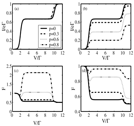
Figure 1: Current (a, b) and Fano factor (c, d) vs. the bias voltage in the P configuration (a, c) and AP configuration (b, d) calculated for no spin-flip processes and different polarization $p$. Other parameters are: $\epsilon_{d}=1$, $U=4$, $T=0.1$.

When the leads are in a P configuration [Fig. 1(a),(c)], an increase of the polarization increases the tunneling rates $\Gamma_{L\uparrow}$ and $\Gamma_{R\uparrow}$ for electrons with the spin-up and decreases the tunneling rates $\Gamma_{L\downarrow}$ and $\Gamma_{R\downarrow}$ for spin-down electrons. This will increase the spin-up current and decrease the spin-down current but it will not affect the total current through the system, which is equal to the sum of the spin-up and spin-down current. In the limit where the Coulomb interaction prevents a double occupancy of the dot, there will be competition between tunneling processes for electrons with the spin-up and those with the spin-down. The characteristic time for these two processes, due to polarization, is unequal: there is fast tunneling of spin-up electrons and slow tunneling of spin-down electrons through the system. The spin which tunnel with a lower rate modulate tunneling of the other spin-direction (so-called dynamical spin-blockade).Cottet1 ; Cottet2 ; Cottet3 Eventually, for a large value of polarization, it leads to an effective bunching of tunneling events and, consequently, to the supper-Poissonian shot noise.

Increasing the bias voltage above the Coulomb blockade regime, i.e, for $eV/2>\epsilon_{d}+U$, opens one more conducting channel and removes spin-blockade. In this regime, spin-up and spin-down electrons are tunneling through the different channels and there is no more competition between these two tunneling events. This leads to a reduction of the current fluctuation and the Fano factor becomes the same as in the paramagnetic case.

The situation is completely different in the AP configuration [Fig. 1(b),(d)]. An increase of the polarization increases tunneling rates $\Gamma_{L\uparrow}$ and $\Gamma_{R\downarrow}$ and decreases tunneling rates $\Gamma_{L\downarrow}$ and $\Gamma_{R\uparrow}$. An electron with the spin-up, which has tunneled from the left electrode into the QD, remains there for a long time because the tunneling rate $\Gamma_{R\uparrow}$ is reduced by the polarization. This decreases the spin-up current. An increase of the polarization also decreases the spin-down current because it reduces the probability for tunneling of the spin-down electrons into the QD. This will decrease a total current through the system. The enhancement of the noise in the AP configuration is due to the asymmetry in the tunneling rates into and out of the QD ($\Gamma_{L\uparrow}>\Gamma_{R\uparrow}$ but $\Gamma_{L\downarrow}<\Gamma_{R\downarrow}$) for each spin separately.

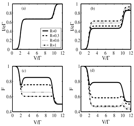
Figure 2: Current (a, b) and Fano factor (c, d) in the P configuration (a, c) and AP configuration (b, d) calculated for polarization $p=0.5$ and different spin-flip processes. Other parameters are the same as in Fig. 1.

For large voltage, in the regime $eV/2>\epsilon_{d}+U$, both conducting channels become available which results in reduction of the noise comparing with the Coulomb blockade regime. In this case the Fano factor does not go to the paramagnetic value because the asymmetry in the tunneling rates are still present.

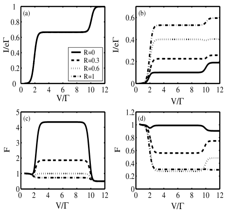
Figure 3: The same as Fig. 2 except for $p=0.9$.

The Fano factor dependence on spin-flip scattering can be analyzed from Figs. 2 and 3. The spin-flip scattering will open one more path in the tunneling of an electron out of the QD: an electron with a spin-up(down) can tunnel into the QD, and due to the spin-flip scattering, it can tunnel out of the QD as an electron with spin-down(up). An electron which was spending more time in QD due to polarization (spin-down in the P configuration and spin-up in the AP configuration) now has more probability to tunnel out from the dot. This causes the decrease of the current fluctuation and Fano factor. However, this is not true for the P-configuration when double occupation of the QD is allowed (for $eV/2>\epsilon_{d}+U$). In this regime the spin-flip does not have any effect on the Fano factor [Figs. 2(c) and 3(c)]. Spin-up and spin-down electrons are passing through separate channels without changing their spins.

V CONCLUSION

In this paper we have analyzed the zero frequency current shot noise through a quantum dot connected to two ferromagnetic leads, taking account for the effects caused by the Coulomb interaction and weak intradot spin-flip scattering. For this purpose the rate equation approach for the description of the shot noise was modified to include the coherent electron evolution inside of the dot. We calculated the Fano factor dependence on the lead configuration (parallel and antiparallel configurations), the degree of their polarization and the amplitude of the spin-flip process. Our results readily show the regimes when the information provided by shot noise measurement will significantly exceed the information which can be obtained from measuring the current.

VI Acknowledgement

This work was supported by the DURINT Program administered by the US Army Research Office. One of the authors, I. Djuric, acknowledges valuable discussions with L. Fedichkin and V. Puller.

References

- (1) Corresponding author e-mail: bdong@stevens.edu
- (2) G.A. Prinz, “Magnetoelectronics,” Science, vol. 282, pp. 1660-1663, 1998.
- (3) S.A. Wolf, D.D. Awschalom, R.A. Buhrman, J.M. Da ughton, S.von Molnar, M.L. Roukes, A.Y. Chtchelkanova, and D.M. Treger, “Spintronics: A Spin-Based Electronics Vision for the Future,” Sience, vol. 294, pp. 1488-1495, 2001.
- (4) J. Barnas̀ and A. Fert, “Magnetoresistance Oscillations due to Charging Effects in Double Ferromagnetic Tunnel Junctions,” Phys. Rev. Lett., vol. 80, pp. 1058-1061, 1998.
- (5) S. Takahashi and S. Maekawa, “Effect of Coulomb Blockade on Magnetoresistance in Ferromagnetic Tunnel Junctions,” Phys. Rev. Lett., vol. 80, pp. 1758-1761, 1998.
- (6) X.H. Wang and A. Brataas, “Large Magnetoresistance Ratio in Ferromagnetic Single-Electron Transistors in the Strong Tunneling Regime,” Phys. Rev. Lett., vol. 83, pp. 5138-5141, 1999.
- (7) D. Mozyrsky, L. Fedichkin, S.A. Gurvitz, and G.P. Berman, “Interference effects in resonant magnetotransport,” Phys. Rev. B, vol. 66, p. 161313, 2002.
- (8) S.I. Erlingsson, and Yu.V. Nazarov, “Hyperfine-mediated transitions between a Zeeman split doublet in GaAs quantum dots: The role of the internal field,” Phys. Rev. B vol. 66, p. 155327, 2002.
- (9) C. Beenakker and C. Schönenberger, “Quantum shot noise,” Phys. Today, vol. 56 (5), pp. 37-42, May 2003.
- (10) For an overview of quantum shot noise, please refer to Ya.M. Blanter and M. Büttiker, “Shot Noise in Mesoscopic Conductors,” Phys. Rep., vol. 336, p. 1, 2000.
- (11) S. Hershfield, J.D. Davies, P. Hyldgaard, C.J. Stanton and J.W. Wilkins, “Zero-frequency current noise for the double-tunnel-junction Coulomb blockade,” Phys. Rev. B, vol. 47, pp. 1967-1979, 1993.
- (12) A.N. Korotkov, “Intrinsic noise of the single-electron transistor,” Phys.Rev. B, vol. 49, pp. 10381-10392, 1994.
- (13) U. Hanke, Yu.M. Galperin, K.A. Chao and Nanzhi Zou, “Finite-frequency shot noise in a correlated tunneling current,” Phys. Rev. B, vol. 48 pp. 17209-17216, 1993
- (14) Yu.V. Nazarov, “Quantum Interference, Tunnel Junctions and Resonant Tunneling,” Physica B, vol. 189, pp. 57-69, 1993.
- (15) S.A. Gurvitz and Ya.S. Prager, “Microscopic derivation of rate equations for quantum transport,” Phys. Rev. B, vol. 53, pp. 15932-15943, 1996.
- (16) Bing Dong, H.L. Cui, and X.L. Lei, “Quantum rate equations for electron transport through an interacting system in the sequential tunneling regime,” Phys. Rev. B, vol. 69, pp. 35324-035339, 2004.
- (17) A. Cottet and W. Belzig, “Dynamical spin-blockade in a quantum dot with paramagnetic leads,” Europhys. Lett., vol. 66, pp. 405-411, 2004.
- (18) A. Cottet, W. Belzig, and C. Bruder, “Positive Cross Correlations in a Three-Terminal Quantum Dot with Ferromagnetic Contacts,” Phys. Rev. Lett., vol. 92, pp. 206801, 2004.
- (19) A. Cottet, W. Belzig, and C. Bruder, “Positive cross-correlations due to Dynamical Channel-Blockade in a three-terminal quantum dot,” cond-mat/0403507, 2004.