Quasiparticle self-energy and many-body effective mass enhancement in a two-dimensional electron liquid

Abstract

Motivated by a number of recent experimental studies we have revisited the problem of the microscopic calculation of the quasiparticle self-energy and many-body effective mass enhancement in a two-dimensional electron liquid. Our systematic study is based on the many-body local fields theory and takes advantage of the results of the most recent Diffusion Monte Carlo calculations of the static charge and spin response of the electron liquid. We report extensive calculations of both the real and imaginary parts of the quasiparticle self-energy. We also present results for the many-body effective mass enhancement and the renormalization constant over an extensive range of electron density. In this respect we critically examine the relative merits of the on-shell approximation versus the self-consistent solution of the Dyson equation. We show that in the strongly-correlated regime a solution of the Dyson equation proves necessary in order to obtain a well behaved effective mass. The inclusion of both charge- and spin-density fluctuations beyond the Random Phase Approximation is indeed crucial to get reasonable agreement with recent measurements.

I Introduction

An interacting electron gas on a uniform neutralizing background (EG) is used as the reference system in most realistic calculations of electronic structure in condensed-matter physics ceperley_1999 . At zero temperature there are only two relevant parameters for a disorder-free EG in the absence of quantizing magnetic fields and spin-orbital coupling: (i) the usual Wigner-Seitz density parameter $r_{s}=(\pi n_{\rm\scriptscriptstyle 2D}a^{2}_{B})^{-1/2}$, $a_{B}=\hbar^{2}{\bar{\kappa}}/(me^{2})$ being the Bohr radius in the medium of interest with ${\bar{\kappa}}$ and $m$ appropriate dielectric constant and bare band mass respectively; and (ii) the degree of spin polarization $\zeta=|n_{\uparrow}-n_{\downarrow}|/n_{\rm\scriptscriptstyle 2D}$. Here $n_{\sigma}$ is the average density of particles with spin $\sigma=\uparrow,\downarrow$ and $n_{\rm\scriptscriptstyle 2D}=n_{\uparrow}+n_{\downarrow}$ is the total average density.

Understanding the many-body aspects of this model has attracted continued interest for many decades singwi_1981 ; march_book . The EG, unlike systems of classical particles, behaves like an ideal paramagnetic gas at high density ($r_{s}\ll 1$) and like a solid at low density wigner ($r_{s}\gg 1$). In the intermediate density regime, which is relevant in three dimensions ($3D$) to conduction electrons in simple metals and in two dimensions ($2D$) to electrons in an inversion layer of a Si metal-oxide-semiconductor field-effect transistor (MOSFET) or in an AlGaAs/GaAs quantum well, perturbative techniques are not effective owing to the lack of a small expansion parameter. One has to take recourse to approximate semi-analytical methods, a number of which have been reviewed in Ref. singwi_1981, , or to Quantum Monte Carlo (QMC) simulation methods ceperley_1980 ; tanatar ; moroni_1992 ; kwon_1994 ; moroni_1995 ; rapisarda ; ortiz ; senatore_1999 ; varsano ; zong ; attaccalite .

Among the methods designed to deal with the intermediate density regime, of particular interest for its physical appeal and elegance is Landau’s phenomenological theory landau dealing with low-lying excitations in a Fermi-liquid. Landau called such single-particle excitations quasiparticles (QP’s) and postulated a one-to-one correspondence between them and the excited states of a non-interacting Fermi gas. He wrote the excitation energy of the Fermi-liquid in terms of the energies of the QP’s and of their effective interactions. The QP-QP interaction function can in turn be used to obtain various physical properties of the system and can be parametrized in terms of experimentally measurable data.

Quinn and Ferrell quinn provided a framework for the microscopic evaluation of the QP-QP interactions in the EG by means of the Random Phase Approximation (RPA). Next, Rice rice incorporated the vertex corrections in the RPA form of the electron self-energy by including the Hubbard hubbard many-body local-field. Some problems in Rice’s theory were subsequently resolved by Ting, Lee, and Quinn ting in their theory of the quasi-$2D$ EG. All these approaches considered only the charge-density fluctuations while neglecting the effect of the spin-density fluctuations.

A more detailed analysis that accounts for the vertex corrections associated with both types of fluctuations was carried out for an unpolarized EG in Refs. vignale_1985, ; zhu_1986, ; yarlagadda_1989, , where Kukkonen-Overhauser-like kukkonen effective interactions were obtained by different approaches. In particular, Yarlagadda and Giuliani yarlagadda_1989 adopted a physically transparent approach termed renormalized Hamiltonian approach (RHA), which will be extensively discussed in this paper. A few electrons from the EG are selected and called “test electrons”, while the remaining EG is treated as a dielectric screening medium. As the test electrons move through this medium, they produce fluctuations in the density of spin-up and spin-down electrons, which provide virtual clothing and also screen their interactions. Thus, the dielectric mimics the true physical processes in an average way. Of course, the test electrons and the electrons of the medium are physically indistinguishable, and this must be taken into account when exchange effects are considered. At this point, after averaging over the coordinates of the screening medium, an effective renormalized Hamiltonian containing only the degrees of freedom of the clothed test electrons (or QP’s) can be derived, under the assumption that the coupling with the medium occurs only via its charge- and spin-density fluctuations. The basic idea underlying the RHA was earlier developed in a beautiful paper by Hamann and Overhauser hamann within the RPA. Calculations based on these theories have been carried out for both $3D$ zhu_1986 ; rahman_1984 and $2D$ santoro_1989 systems.

In a parallel theoretical development Ng and Singwi ng , starting from a Ward identity and performing a local approximation on the irreducible particle-hole interaction, obtained an expression for the self-energy in terms of the many-body local field factors associated with charge- and spin-density fluctuations. Equivalent results were later obtained by Yarlagadda and Giuliani yarlagadda_1994 ; yarlagadda_gstar by means of the RHA. These authors also took into account an infinitesimal degree of spin polarization which allowed them to carry out calculations of the Landau Fermi-liquid parameters.

The previous theoretical work suffers from two major shortcomings. (i) All available earlier calculations have adopted a static and oversimplified Hubbard-like model for the local-field factors, which do not have the appropriate behavior at both intemediate and large wave number $q$. We have corrected for these discrepancies (while still neglecting the frequency dependence of the local fields) using recent parametrizations davoudi_2001 for the static local fields of a $2D$ EG. (ii) The RHA briefly introduced above is an “on-shell” theory (see Sect. II.2) and, as we will show in this work, predicts a divergence of the effective mass with decreasing electron density. In the spirit of the work of Santoro-Giuliani santoro_1989 and of Ng-Singwi ng we have kept in this work the full frequency dependence of the self-energy and carried out a self-consistent solution of the Dyson equation to find the proper QP excitation energy and QP properties. Comparing with Ref. santoro_1989, , we have released the plasmon$+$paramagnon-pole approximation to the charge-charge and spin-spin response functions.

From the experimental point of view, as already remarked, electrons in a semiconductor inversion layer or in a quantum well can be modelled by a quasi-$2D$ EG ando . Quantum Shubnikov-de Haas (SdH) oscillations of the magnetoresistance abrikosov provide a powerful tool for measuring Fermi-liquid parameters of a quasi-$2D$ EG. Measurements performed over the past years smith ; abstreiter ; fang ; neugebauer have shown sizeable renormalizations of the QP effective mass and effective Landé $g$-factor. These experiments have been performed in a relatively high-density regime, i.e. for $r_{s}\lesssim 2$ say. The density dependence of the effective mass $m^{*}$ was obtained by Smith and Stiles smith from a study of SdH oscillations in Si inversion layers. To obtain the same information Abstreiter et al. abstreiter used instead cyclotron resonance measurements. Fang and Stiles fang and Neugebauer et al. neugebauer performed a series of SdH experiments on Si inversion layers and obtained the dependence of the modified Landé factor $g^{*}$ on carrier density. The product of $g^{*}$ and $m^{*}$, which is proportional to the spin susceptibility $\chi_{S}$, can be determined from the SdH oscillations in a tilted magnetic field as suggested in Ref. fang, .

The issue of the apparent metal-insulator transition mit (MIT) in low-density $2D$ electron systems has prompted intense experimental studies on quasiparticle properties dolgopolov ; okamoto ; vitkalov ; shashkin ; pudalov_prl ; tutuc ; noh ; zhu_2003 ; vakili_2004 in the intermediate-to-strong coupling regime, $r_{s}\gtrsim 2$ say. Many authors dolgopolov have shown that the resistance of a Si-MOSFET is increased dramatically by increasing the value of an in-plane magnetic field, and saturates at a characteristic value of several Tesla. Performing low-field SdH measurements on Si-MOSFET’s, Okamoto et al. okamoto have shown that the saturation value is the magnetic field that is necessary to fully polarize the electron spins. An interpretation vitkalov ; shashkin of the in-plane magnetoresistance in Si inversion layers suggested a ferromagnetic instability at or very close to the critical density for the $2D$ MIT driven by a divergence in the effective mass. Direct measurements of $m^{*}$ in high-mobility Si-MOSFET’s over a wide range of carrier density, using a novel technique based on the beating pattern of SdH oscillations in crossed magnetic fields, have been reported by Pudalov et al. pudalov_prl . These authors measured $m^{*}$ and $\chi_{S}$ in the vicinity of the $2D$ MIT, but found no evidence for a divergent behavior. Only a moderate enhancement of $m^{*}$ by a factor of $\approx 2-2.5$ over the band mass was observed near the critical density for the $2D$ MIT. Two groups have also reported anomalous density dependences of the Landé factor in $n$-doped tutuc ($2\lesssim r_{s}\lesssim 7$) and $p$-doped noh ($r_{s}\gtrsim 17$) GaAs/AlGaAs heterojunctions that are in disagreement with results in Si-MOSFET’s. The dependence of the spin susceptibility on the degree of spin polarization of the sample can account for this anomalous behavior as pointed out by Zhu et al. zhu_2003 , who studied a $2D$ EG of exceedingly high quality.

To complete the cornucopia of recent experimental findings on QP properties, it is worth mentioning that Vakili et al. vakili_2004 have reported measurements of $m^{*}$ and $\chi_{S}$ in a dilute $2D$ EG confined to a narrow AlAs quantum well (only $45\,{\rm\AA}$ wide). The electron system investigated in Ref. vakili_2004, is quite interesting because the electrons occupy an out-of-plane conduction-band valley, rendering the system similar to $2D$ electrons in Si-MOSFET’s but with only one valley occupied. Quite surprisingly, the results of Vakili et al. vakili_2004 for $\chi_{S}$ are in good agreement with the QMC results of Attaccalite et al. attaccalite even though this simulation has been carried out for a strictly disorder-free EG. This might indicate that $\chi_{S}$ is not strongly dependent on disorder. On the other hand, there is a significant spread in the experimental results of Ref. vakili_2004, for $m^{*}$, which turns out to be both sample and cool-down dependent. Difficulties associated with the SdH data analysis have been pointed out in Ref. vakili_2004, as one of the possible causes for this spread.

At this point it is probably worth commenting that indeed there could be in principle subtle issues associated with the analysis of the SdH traces in $2D$ systems. In fact the amplitude of the SdH oscillations is usually fitted to the $3D$ Lifshitz-Kosevich (LK) formula lk upon a trivial change in the single-particle spectrum. The fit is based on an impurity scattering Dingle temperature $T_{D}$ and an “effective” mass. In recent years a number of caveats concerning the applicability of such a procedure to $2D$ strongly-interacting systems have appeared caveats . In particular, Martin et al. maslov have shown that the interplay between electron-electron interactions and electron-impurity scattering leads in $2D$ to an effective temperature-dependent Dingle temperature with a leading low-temperature behavior of the type $T_{D}(T)\propto T\ln{T}$. The need for the introduction of a temperature-dependent Dingle parameter in strongly-coupled Si-MOSFET’s has been emphasized in the above-mentioned Ref. pudalov_prl where a linear $T_{D}(T)$ was used to fit the longitudinal magnetoresistance data. Quantitative differences on the resultant effective mass are found using such type of procedure: roughly speaking, the tendency is to get substantially lower values for $m^{*}$ than those obtained using the same Dingle parameter for all temperatures.

For a quantitative comparison between suitable theories that take into account quasi-$2D$ effects (such as finite width of the electron wavefunctions in the confinement direction and valley degeneracies) and the experimental results smith ; fang for Si-MOSFET’s in the weak-coupling regime $r_{s}\lesssim 2$ we refer the reader to the work of Yarlagadda and Giuliani yarlagadda_gstar and references therein. In this work we will try and carry out a comparison between the theory and the experimental data of Zhu et al. private_zhu for strongly-interacting electrons ($2\lesssim r_{s}\lesssim 6$), occupying a single valley in an exceptionally clean GaAs/AlGaAs quantum well.

The contents of the paper are described briefly as follows. In Sect. II we present in great detail the theoretical background. We proceed in Sect. III to discuss the inputs we have used for our numerical calculations, while in Sect. IV we present our main results for the real and imaginary part of the quasiparticle self-energy, the many-body enhancement of the effective mass, and the renormalization constant. Finally, in Sect. V we compare our theory with the experimental results of Zhu et al. private_zhu and report some conclusions. In order to make the paper fully self-contained we have included two Appendices which contain a number of helpful details on how we have in practice calculated the QP self-energy.

II Theory of the quasiparticle self-energy

The aim of this Section is to give a sound theoretical justification to the expression for the retarded QP self-energy $\Sigma_{\rm\scriptstyle ret}({\bf k},\omega)$ of a $2D$ paramagnetic EG that will be used throughout this paper and that we have summarized in Eqs. (3) and (7) below.

To fix the notation we start by introducing the Hamiltonian for a $2D$ EG confined to an area $S$,

$${\mathcal{H}}_{\rm EG}=\sum_{{\bf k},\sigma}\varepsilon_{\bf k}{\hat{c}}^{\dagger}_{{\bf k},\sigma}{\hat{c}}_{{\bf k},\sigma}+\frac{1}{2S}\sum_{{\bf q}\neq 0}v_{\bf q}\sum_{{\bf k}_{1},\sigma_{1}}\sum_{{\bf k}_{2},\sigma_{2}}{\hat{c}}^{\dagger}_{{\bf k}_{1}+{\bf q},\sigma_{1}}{\hat{c}}^{\dagger}_{{\bf k}_{2}-{\bf q},\sigma_{2}}{\hat{c}}_{{\bf k}_{2},\sigma_{2}}{\hat{c}}_{{\bf k}_{1},\sigma_{1}}\,.$$ (1)

Here ${\hat{c}}^{\,\dagger}_{{\bf k},\,\sigma}$ and ${\hat{c}}_{{\bf k},\,\sigma}$ are fermionic creation and annihilation operators which satisfy canonical anticommutation relations, $\varepsilon_{\bf k}=\hbar^{2}{\bf k}^{2}/(2m)$ is the single-particle energy, and $v_{\bf q}=2\pi e^{2}/q$ is the $2D$ Fourier transform of the bare Coulomb interaction $e^{2}/r$. For later purposes we introduce the Fermi wave number $k_{F}=(2\pi n_{\rm\scriptscriptstyle 2D})^{1/2}=\sqrt{2}/(r_{s}a_{B})$, the Fermi energy $\varepsilon_{F}=\hbar^{2}k^{2}_{F}/(2m)$ and the quantity $\xi_{\bf k}=\varepsilon_{\bf k}-\varepsilon_{F}$.

The retarded QP self-energy $\Sigma_{\rm\scriptstyle ret}({\bf k},\omega)$ is written as the sum of two terms,

$$\Sigma_{\rm\scriptstyle ret}({\bf k},\omega)=\Sigma_{\rm\scriptstyle SX}({\bf k},\omega)+\Sigma_{\rm\scriptstyle CH}({\bf k},\omega)$$ (2)

where the first term is called “screened-exchange” (SX) and the second term is called “Coulomb-hole” (CH). The frequency $\omega$ is measured from $\varepsilon_{F}/\hbar$.

The SX contribution is given by

$$\Sigma_{\rm\scriptstyle SX}({\bf k},\omega)=-\int\frac{d^{2}{\bf q}}{(2\pi)^{2}}\,\frac{v_{\bf q}}{\varepsilon({\bf q},\omega-\xi_{{\bf k}+{\bf q}}/\hbar)}\,\Theta(-\xi_{{\bf k}+{\bf q}}/\hbar)\,.$$ (3)

Here $\Theta(x)$ is the step function and $\varepsilon({\bf q},\omega)$ is a screening function originating from effective Kukkonen-Overhauser interactions kukkonen ,

$$\frac{1}{\varepsilon({\bf q},\omega)}=1+v_{\bf q}\,\left[1-G_{+}({\bf q},\omega)\right]^{2}\,\chi_{\rm\scriptstyle C}({\bf q},\omega)+3\,v_{\bf q}\,G^{2}_{-}({\bf q},\omega)\,\chi_{\rm\scriptstyle S}({\bf q},\omega)\,.$$ (4)

In Eq. (4) the charge-charge and spin-spin response functions $\chi_{\rm\scriptstyle C}({\bf q},\omega)$ and $\chi_{\rm\scriptstyle S}({\bf q},\omega)$ are determined by the spin-symmetric and spin-antisymmetric local-field factors $G_{+}({\bf q},\omega)$ and $G_{-}({\bf q},\omega)$,

$$\chi_{\rm\scriptstyle C}({\bf q},\omega)=\frac{\chi_{0}({\bf q},\omega)}{1-v_{\bf q}[1-G_{+}({\bf q},\omega)]\chi_{0}({\bf q},\omega)}$$ (5)

and

$$\chi_{\rm\scriptstyle S}({\bf q},\omega)=\frac{\chi_{0}({\bf q},\omega)}{1+v_{\bf q}G_{-}({\bf q},\omega)\,\chi_{0}({\bf q},\omega)}\,,$$ (6)

$\chi_{0}({\bf q},\omega)$ being the Stern response function of a noninteracting $2D$ EG stern_1967 . In the paramagnetic electron liquid $G_{\pm}({\bf q},\omega)=[G_{\uparrow\uparrow}({\bf q},\omega)\pm G_{\uparrow\downarrow}({\bf q},\omega)]/2$, where $G_{\sigma\sigma^{\prime}}({\bf q},\omega)$ are the spin-resolved local fields. Note that $\Sigma_{\rm\scriptstyle SX}({\bf k},\omega)$ is just an ordinary exchange-like self-energy built from the Kukkonen-Overhauser effective interactions instead of bare Coulomb interactions, which would lead to the frequency-independent Hartree-Fock self-energy first calculated for the $2D$ EG by Stern stern_1973 .

The CH contribution to the retarded self-energy is given by

$$\Sigma_{\rm\scriptstyle CH}({\bf k},\omega)=-\int\frac{d^{2}{\bf q}}{(2\pi)^{2}}\,v_{\bf q}\int_{0}^{+\infty}\,\frac{d\Omega}{\pi}\,\,\frac{\Im m[\varepsilon^{-1}({\bf q},\Omega)]}{\omega-\xi_{{\bf k}+{\bf q}}/\hbar-\Omega+i\delta}\,,$$ (7)

where $\delta$ is a positive infinitesimal. The real and imaginary part of the retarded self-energy are readily obtained from Eqs. (3) and (7) with the result

$$\Re e\Sigma_{\rm\scriptstyle ret}({\bf k},\omega)= - \int\frac{d^{2}{\bf q}}{(2\pi)^{2}}\,v_{\bf q}\Re e[\varepsilon^{-1}({\bf q},\omega-\xi_{{\bf k}+{\bf q}}/\hbar)]\,\Theta(-\xi_{{\bf k}+{\bf q}}/\hbar)$$

$$- \int\frac{d^{2}{\bf q}}{(2\pi)^{2}}\,v_{\bf q}{\mathcal{P}}\int_{0}^{+\infty}\,\frac{d\Omega}{\pi}\,\frac{\Im m[\varepsilon^{-1}({\bf q},\Omega)]}{\omega-\xi_{{\bf k}+{\bf q}}/\hbar-\Omega}\,,$$

and

$$\Im m\Sigma_{\rm\scriptstyle ret}({\bf k},\omega)=\int\frac{d^{2}{\bf q}}{(2\pi)^{2}}\,v_{\bf q}\Im m[\varepsilon^{-1}({\bf q},\omega-\xi_{{\bf k}+{\bf q}}/\hbar)]\left[\Theta(\omega-\xi_{{\bf k}+{\bf q}}/\hbar)-\Theta(-\xi_{{\bf k}+{\bf q}}/\hbar)\right]\,.$$ (9)

Once the QP self-energy is known, the QP excitation energy $\delta{\mathcal{E}}_{\rm QP}({\bf k})$, which is the QP energy measured from the chemical potential $\mu$ of the interacting EG, can be calculated by solving self-consistently the Dyson equation

$$\delta{\mathcal{E}}_{\rm QP}({\bf k}) = \xi_{\bf k}+\left.\Re e\Sigma^{\rm R}_{\rm\scriptstyle ret}({\bf k},\omega)\right|_{\omega=\,\delta{\mathcal{E}}_{\rm QP}({\bf k})/\hbar}\,,$$ (10)

where $\Re e\Sigma^{\rm R}_{\rm\scriptstyle ret}({\bf k},\omega)=\Re e\Sigma_{\rm\scriptstyle ret}({\bf k},\omega)-\Sigma_{\rm\scriptstyle ret}(k_{F},0)$. For later purposes we introduce at this point the so-called on-shell approximation (OSA). This amounts to approximating the QP excitation energy by calculating $\Re e\Sigma^{\rm R}_{\rm\scriptstyle ret}({\bf k},\omega)$ in Eq. (10) at the frequency $\omega=\xi_{\bf k}/\hbar$ corresponding to the single-particle energy, that is

$$\delta{\mathcal{E}}_{\rm QP}({\bf k})\simeq\xi_{\bf k}+\left.\Re e\Sigma^{\rm R}_{\rm\scriptstyle ret}({\bf k},\omega)\right|_{\omega=\xi_{\bf k}/\hbar}\,.$$ (11)

In Sects. II.1 and II.2 we will give a formal justification of Eqs. (3) and (7) using two completely different methods: diagrammatic perturbation theory (Sect. II.1) and renormalized Hamiltonian approach (Sect. II.2). In the following we shall soon drop, however, the frequency dependence of the local-field factors. Recent studies nifosi have evaluated it in the long-wavelength limit ${\bf q}\rightarrow 0$, but the knowledge of the full dependence on wave number is necessary for the type of calculations that we are interested in.

II.1 Diagrammatic perturbation theory

In this Section we use a diagrammatic approach that was first developed by Ng and Singwi ng , building on earlier ideas by Vignale and Singwi vignale_1985 . The starting point is the identity nozieres

$$\delta\Sigma_{\sigma}({\bf k},\omega)=i\sum_{\sigma^{\prime}}\int\frac{d^{2}{\bf k}^{\prime}d\omega^{\prime}}{(2\pi)^{3}}I_{{\bf k}\omega\sigma,{\bf k}^{\prime}\omega^{\prime}\sigma^{\prime}}(0)\delta G_{\sigma^{\prime}}({\bf k}^{\prime},\omega^{\prime})~{},$$ (12)

where $\delta\Sigma_{\sigma}({\bf k},\omega)$ and $\delta G_{\sigma}({\bf k},\omega)$ are infinitesimal changes in the self-energy and the Green’s function, and $I_{{\bf k}\omega\sigma,{\bf k}^{\prime}\omega^{\prime}\sigma^{\prime}}(0)$ is the irreducible electron-hole interaction at zero momentum and energy transfer. This identity is graphically represented in Fig. 1. The defining feature of the irreducible electron-hole scattering block $I$ is that it includes only diagrams that cannot be divided into two parts by cutting a single electron-hole pair propagator carrying zero energy and momentum.

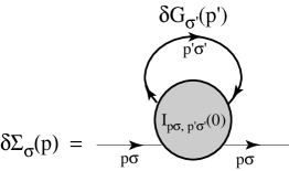
Figure 1: Diagrammatic representation of the identity (12). Here and in the following we use the four-momentum variable $p$ as a shorthand for $({\bf k},\omega)$.

The differential relation (12) cannot be integrated as it stands because $I$ is a complicated functional of $G$. The idea of Ng and Singwi was to use an approximate form of $I_{{\bf k}\omega\sigma,{\bf k}^{\prime}\omega^{\prime}\sigma^{\prime}}(0)$ that does not depend on $G$. The “local approximation” introduced by Vignale and Singwi in their study of the effective electron-electron interaction vignale_1985 is useful for this purpose since it yields by physical arguments an expression of the form

$$I_{{\bf k}\omega\sigma,{\bf k}^{\prime}\omega^{\prime}\sigma^{\prime}}(0)\simeq V^{\rm eff}_{\sigma\sigma^{\prime}}({\bf k}-{\bf k}^{\prime},\omega-\omega^{\prime})~{},$$ (13)

where $V^{\rm eff}_{\sigma\sigma^{\prime}}$ is just a function of the momentum and energy transfers in the electron-hole channel. Thus the main characteristic of the Ng-Singwi approach is that the key approximation in Eq. (13) is made on the irreducible electron-hole interaction rather than on the self-energy itself. With this approximation we can integrate Eq. (12) and obtain, up to an integration constant, the result

$$\Sigma_{\sigma}({\bf k},\omega)=i\sum_{\sigma^{\prime}}\int\frac{d^{2}{\bf k}^{\prime}d\omega^{\prime}}{(2\pi)^{3}}V^{\rm eff}_{\sigma\sigma^{\prime}}({\bf k}-{\bf k}^{\prime},\omega-\omega^{\prime})G_{\sigma^{\prime}}({\bf k}^{\prime},\omega^{\prime})~{}.$$ (14)

With the replacements ${\bf k}-{\bf k}^{\prime}={\bf q}$ and $\omega-\omega^{\prime}=\Omega$, this expression has the form of the GW approximation hedin except for two crucial differences: (i) the effective interaction $V^{\rm eff}_{\sigma\sigma^{\prime}}({\bf q},\Omega)$ includes vertex corrections and is therefore more general than the screened interaction $W({\bf q},\Omega)$ between test charges that appears in the GW approximation; and (ii) the expression (14) involves an undetermined integration constant which must be fixed by independent means, for example by requiring that $\Sigma(k_{F},0)$ reproduces the correct value of the chemical potential as determined from QMC data. An analytic continuation procedure allows one to recast the time-ordered self-energy in Eq. (14) into a retarded self-energy given by the sum of SX and CH contributions as in Eq. (2).

In their derivation of the “local approximation” in Eq. (13) Ng and Singwi sorted the diagrams that contribute to the irreducible electron-hole interaction into three classes: (1) diagrams that are reducible in the “crossed” particle-hole channel, carrying momentum ${\bf q}$ and energy $\Omega$; (2) diagrams that are reducible in the particle-particle channel; and (3) diagrams that are irreducible in the particle-particle channel and in both particle-hole channels. The diagrams of class (1) are shown in Fig. 2.

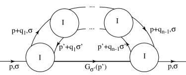
Figure 2: Structure of the diagrams included in the approximate evaluation of $I_{p\sigma,p^{\prime}\sigma^{\prime}}(0)$. The number of irreducible interaction blocks is $n\geq 2$, and there is an integral over the internal four-momenta $q_{1},...,q_{n-1}$. Notice that these diagrams are reducible in the particle-hole channel that carries four-momentum $p-p^{\prime}$, but irreducible in the particle-hole channel defined by the two external legs, which carries zero four-momentum. The irreducible interaction blocks are further analyzed in Fig. 3.

Notice that these diagrams are expressed in terms of three building blocks as shown in Fig. 3, which are irreducible in the “crossed” particle-hole channel.

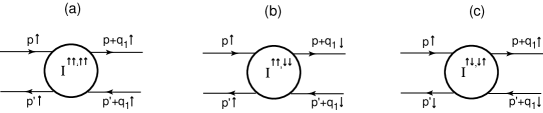
Figure 3: The three irreducible blocks out of which the “railroad diagrams” of Fig. 2 are constructed.

In block (a) the particle and the hole have parallel spin orientations which are conserved as they scatter against each other. In block (b) the particle and the hole have parallel spin orientations, which are reversed as a result of the scattering process. Finally, in block (c) the particle and the hole have opposite spin orientations.

In order to make further progress we now approximate these irreducible blocks by functions of the electron-hole momentum ${\bf q}={\bf k}-{\bf k}^{\prime}$. The form of these functions is determined by requiring that the same approximation, when applied to the evaluation of the diagrams for the density-density and spin-spin response functions, yields Eqs. (5) and (6). For the two diagrams 3(a) and 3(b) this is accomplished by setting

$$I^{\sigma\sigma,\tau\tau}\simeq v_{{\bf q}}[1-G_{\sigma\tau}({\bf q})]~{},$$ (15)

where $\sigma$ and $\tau$ are the spin orientations of the particle and of the hole before and after scattering (the labelling is explained in Fig. 3). For diagram 3(c) a simple reasoning based on isotropy in spin space for the paramagnetic state leads to

$$I^{\sigma\bar{\sigma},\bar{\sigma}\sigma}=I^{\sigma\sigma,\sigma\sigma}-I^{\sigma\sigma,\bar{\sigma}\bar{\sigma}}\simeq-2v_{{\bf q}}G_{-}({\bf q})~{},$$ (16)

as one can see from Fig. 4.

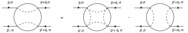
Figure 4: Graphical illustration of the relationship between different components of the irreducible electron-hole scattering amplitude in a spin-unpolarized state.

The integrals over the internal four-momenta in Fig. 2 can be carried out analytically if the intermediate Green’s functions are replaced by noninteracting Green’s functions, giving a result proportional to $[\chi_{0}(p-p^{\prime})]^{n}$ where $\chi_{0}$ is the Stern function. The whole series of diagrams can then be summed algebraically yielding

$$V^{{\rm eff},(1)}_{\sigma\sigma^{\prime}}({\bf q},\Omega) = [v_{{\bf q}}G_{+}({\bf q})]^{2}\chi_{C}({\bf q},\Omega)\delta_{\sigma,\sigma^{\prime}}+[v_{{\bf q}}G_{-}({\bf q})]^{2}\chi_{S}({\bf q},\Omega)\delta_{\sigma,\sigma^{\prime}}$$ (17)

$$+ 2[v_{{\bf q}}G_{-}({\bf q})]^{2}\chi_{S}({\bf q},\Omega)\delta_{\sigma,-\sigma^{\prime}}~{}.$$

The subscripts $+$ and $-$ denote as usual the charge and the longitudinal spin channels. The density-density and spin-spin response functions are expressed in terms of the Stern function and of the many-body local field factors according to Eqs. (5) and (6).

The evaluation of the remaining terms, i.e. the particle-particle ladder diagrams and the fully irreducible diagrams, is considerably more complex. The only simple diagram is the bare exchange interaction with momentum transfer ${\bf q}$, which yields the Hartree-Fock self-energy. All other terms are dropped in the possibly naive hope that they are smaller than the terms retained in Eq. (17). Keeping only the bare exchange interaction and combining it with Eq. (17) we arrive at an effective interaction of the form

$$\left\{\begin{array}[]{l}V^{\rm eff}_{\uparrow\uparrow}({\bf q},\Omega)=v_{\bf q}+\{v_{\bf q}[1-G_{+}({\bf q})]\}^{2}\chi_{C}({\bf q},\Omega)+[v_{\bf q}G_{-}({\bf q})]^{2}\chi_{S}({\bf q},\Omega)\\ V^{\rm eff}_{\uparrow\downarrow}({\bf q},\Omega)=2[v_{\bf q}G_{-}({\bf q})]^{2}\chi_{S}({\bf q},\Omega)~{}.\end{array}\right.$$ (18)

Inserting this in Eq. (14) and repeating standard analytical transformations hedin one easily recovers the expressions (3) and (7) for the screened-exchange and Coulomb-hole contributions to the self-energy.

Let us emphasize again that the result that we have obtained by a diagrammatic method rests on Eq. (14) for the self-energy (apart from an additive constant) and on the use of the effective interactions shown in Eq. (18). It should be evident from the above derivation that no diagram for $I_{{\bf k}\omega\sigma,{\bf k}^{\prime}\omega^{\prime}\sigma^{\prime}}(0)$ has been double-counted. Rather, many diagrams have been dropped, but the result for the self-energy remains to be adjusted a posteriori by fixing the addivite constant through the correct value of the chemical potential.

Let us see, on the other hand, what would have happened if we had applied the local approximation directly to the self-energy starting from the alternative exact expression,

$$\Sigma_{\sigma}({\bf k},\omega)=i\sum_{\sigma^{\prime}}\int\frac{d^{2}{\bf k}^{\prime}d\omega^{\prime}}{(2\pi)^{3}}\frac{v_{{\bf k}-{\bf k}^{\prime}}}{\epsilon({\bf k}-{\bf k}^{\prime},\omega-\omega^{\prime})}\tilde{\Lambda}_{{\bf k}\omega,{\bf k}^{\prime}\omega^{\prime}}G_{\sigma^{\prime}}({\bf k}^{\prime},\omega^{\prime})~{},$$ (19)

where $\tilde{\Lambda}$ is the proper vertex function and $\epsilon$ is the regular dielectric function (see Fig. 5). Within the local approximation one finds rice ; rahman_1984 ; mahan_1989

$$\tilde{\Lambda}_{{\bf k}\omega,{\bf k}^{\prime}\omega^{\prime}}=\frac{1}{1+v_{{\bf k}-{\bf k}^{\prime}}G_{+}({\bf k}-{\bf k}^{\prime})\chi_{0}({\bf k}-{\bf k}^{\prime},\omega-\omega^{\prime})}~{},$$ (20)

so that this route to the self-energy includes only the contribution of charge fluctuations but misses completely that of spin fluctuations. The root of the difficulty obviously lies in the fact that the local approximation for the vertex function is not good enough to capture the contribution of spin-density fluctuations. On the other hand, the dependence of $I$ on spin fluctuations is manifest in the terms proportional to $G_{-}^{2}$ in Eq. (17). This is the main physical reason why it is better to apply the local approximation to the differential relation (12) than to the integral relation (19). In fact, all quasiparticle properties of our present interest depend on relative variations of the self-energy, i.e. on $\delta\Sigma$ rather than on the absolute value of $\Sigma$.

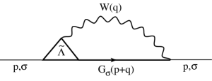
Figure 5: Diagrammatic representation of Eq. (19). Here $W({\bf q},\Omega)=v_{\bf q}/\epsilon({\bf q},\Omega)$ is the usual test charge-test charge screened interaction.

II.2 Renormalized Hamiltonian approach

In this Section we discuss the derivation of Eqs. (3) and (7) from the point of view of an effective renormalized Hamiltonian for the low-energy degrees of freedom of the electron liquid yarlagadda_1989 ; yarlagadda_1994 ; yarlagadda_gstar .

We start by dividing the Hilbert space of the EG Hamiltonian ${\mathcal{H}}_{\rm EG}$ reported in Eq. (1) into a “slow” sector (${\mathcal{S}}_{\Lambda}$) and a “fast” sector (${\mathcal{F}}_{\Lambda}$), assuming the existence of the Fermi surface at $k=k_{F}$. ${\mathcal{S}}_{\Lambda}$ contains only plane-wave states with wavevector ${\bf k}$ close to the Fermi surface, i.e. such that $|k-k_{F}|<\Lambda$ where $\Lambda$ is an arbitrarily small cutoff. ${\mathcal{F}}_{\Lambda}$ contains all the other states. We correspondingly introduce “slow” and “fast” creation and annihilation operators which operate in these two sectors,

$${\hat{c}}_{{\bf k},\sigma}=\left\{\begin{array}[]{l}{\hat{s}}_{{\bf k},\sigma},\,\,{\bf k}\in{\mathcal{S}}_{\Lambda}\,,\\ {\hat{f}}_{{\bf k},\sigma},\,\,{\bf k}\in{\mathcal{F}}_{\Lambda}\,.\end{array}\right.$$ (21)

Our aim is to derive an effective Hamiltonian for the slow sector which contains only the ${\hat{s}}_{{\bf k},\sigma}$ operators by integrating out in a reasoned manner the ${\hat{f}}_{{\bf k},\sigma}$ degrees of freedom.

${\mathcal{H}}_{\rm EG}$ is first rewritten using the ${\hat{s}}_{{\bf k},\sigma}$ and ${\hat{f}}_{{\bf k},\sigma}$ operators,

$${\mathcal{H}}_{\rm EG}={\mathcal{H}}_{\rm s}+{\mathcal{H}}_{\rm f}+{\mathcal{H}}_{\rm sf}\,.$$ (22)

The first term is

$${\mathcal{H}}_{\rm s}=\sum_{{\bf k},\sigma}\varepsilon_{\bf k}{\hat{s}}^{\dagger}_{{\bf k},\sigma}{\hat{s}}_{{\bf k},\sigma}+\frac{1}{2S}\sum_{{\bf q}\neq 0}v_{\bf q}\sum_{{\bf k}_{1},\sigma_{1}}\sum_{{\bf k}_{2},\sigma_{2}}{\hat{s}}^{\dagger}_{{\bf k}_{1}+{\bf q},\sigma_{1}}{\hat{s}}^{\dagger}_{{\bf k}_{2}-{\bf q},\sigma_{2}}{\hat{s}}_{{\bf k}_{2},\sigma_{2}}{\hat{s}}_{{\bf k}_{1},\sigma_{1}}\,,$$ (23)

where all wavevectors belong to ${\mathcal{S}}_{\Lambda}$. Note that the second term in ${\mathcal{H}}_{\rm s}$, which represents the direct interaction between slow particles, tends to zero faster than the kinetic energy term in the limit $\Lambda\rightarrow 0$. Thus this term will be treated by first-order perturbation theory below.

The second term in Eq. (22) is the Hamiltonian for the fast sector,

$${\mathcal{H}}_{\rm f}=\sum_{{\bf k},\sigma}\varepsilon_{\bf k}{\hat{f}}^{\dagger}_{{\bf k},\sigma}{\hat{f}}_{{\bf k},\sigma}+\frac{1}{2S}\sum_{{\bf q}\neq 0}v_{\bf q}\sum_{{\bf k}_{1},\sigma_{1}}\sum_{{\bf k}_{2},\sigma_{2}}{\hat{f}}^{\dagger}_{{\bf k}_{1}+{\bf q},\sigma_{1}}{\hat{f}}^{\dagger}_{{\bf k}_{2}-{\bf q},\sigma_{2}}{\hat{f}}_{{\bf k}_{2},\sigma_{2}}{\hat{f}}_{{\bf k}_{1},\sigma_{1}}$$ (24)

where all wavevectors belong to ${\mathcal{F}}_{\Lambda}$. ${\mathcal{H}}_{\rm f}$ tends to the full EG Hamiltonian in the limit $\Lambda\rightarrow 0$ and this property will be useful in what follows.

The third term ${\mathcal{H}}_{\rm sf}$ describes the interaction between the slow and the fast particles: this term is the sum of fourteen different terms, but here we assume that the relevant operators are those which separately conserve the number of particles in the two sectors, i.e. terms of the type ${\hat{s}}^{\dagger}_{{\bf k}_{1}+{\bf q},\sigma_{1}}{\hat{s}}^{\dagger}_{{\bf k}_{2}-{\bf q},\sigma_{2}}{\hat{s}}_{{\bf k}_{2},\sigma_{2}}{\hat{f}}_{{\bf k}_{1},\sigma_{1}}$ (trilinear in the field operators of either slow or fast particles) or ${\hat{s}}^{\dagger}_{{\bf k}_{1}+{\bf q},\sigma_{1}}{\hat{s}}^{\dagger}_{{\bf k}_{2}-{\bf q},\sigma_{2}}{\hat{f}}_{{\bf k}_{2},\sigma_{2}}{\hat{f}}_{{\bf k}_{1},\sigma_{1}}$ will be dropped. Four terms are left within this assumption,

$${\mathcal{H}}_{\rm sf} \simeq \frac{1}{2S}\sum_{{\bf q}\neq 0}v_{\bf q}\sum_{{\bf k}_{1},\sigma_{1}}\sum_{{\bf k}_{2},\sigma_{2}}{\hat{s}}^{\dagger}_{{\bf k}_{1}+{\bf q},\sigma_{1}}{\hat{f}}^{\dagger}_{{\bf k}_{2}-{\bf q},\sigma_{2}}{\hat{f}}_{{\bf k}_{2},\sigma_{2}}{\hat{s}}_{{\bf k}_{1},\sigma_{1}}$$ (25)

$$+ \frac{1}{2S}\sum_{{\bf q}\neq 0}v_{\bf q}\sum_{{\bf k}_{1},\sigma_{1}}\sum_{{\bf k}_{2},\sigma_{2}}{\hat{f}}^{\dagger}_{{\bf k}_{1}+{\bf q},\sigma_{1}}{\hat{s}}^{\dagger}_{{\bf k}_{2}-{\bf q},\sigma_{2}}{\hat{s}}_{{\bf k}_{2},\sigma_{2}}{\hat{f}}_{{\bf k}_{1},\sigma_{1}}$$

$$+ \frac{1}{2S}\sum_{{\bf q}\neq 0}v_{\bf q}\sum_{{\bf k}_{1},\sigma_{1}}\sum_{{\bf k}_{2},\sigma_{2}}{\hat{s}}^{\dagger}_{{\bf k}_{1}+{\bf q},\sigma_{1}}{\hat{f}}^{\dagger}_{{\bf k}_{2}-{\bf q},\sigma_{2}}{\hat{s}}_{{\bf k}_{2},\sigma_{1}}{\hat{f}}_{{\bf k}_{1},\sigma_{2}}$$

$$+ \frac{1}{2S}\sum_{{\bf q}\neq 0}v_{\bf q}\sum_{{\bf k}_{1},\sigma_{1}}\sum_{{\bf k}_{2},\sigma_{2}}{\hat{f}}^{\dagger}_{{\bf k}_{1}+{\bf q},\sigma_{1}}{\hat{s}}^{\dagger}_{{\bf k}_{2}-{\bf q},\sigma_{2}}{\hat{f}}_{{\bf k}_{2},\sigma_{1}}{\hat{s}}_{{\bf k}_{1},\sigma_{2}}$$

where ${\bf k}_{1}$ and ${\bf k}_{1}+{\bf q}$ belong to ${\mathcal{S}}_{\Lambda}$, and ${\bf k}_{2}$ and ${\bf k}_{2}-{\bf q}$ belong to ${\mathcal{F}}_{\Lambda}$. By simple algebraic manipulations ${\mathcal{H}}_{\rm sf}$ can be written as

$${\mathcal{H}}_{\rm sf} = \frac{1}{S}\sum_{{\bf q}\neq 0}\sum_{{\bf k}_{1},\sigma_{1}}\sum_{{\bf k}_{2},\sigma_{2}}v_{\bf q}{\hat{s}}^{\dagger}_{{\bf k}_{1}+{\bf q},\sigma_{1}}{\hat{f}}^{\dagger}_{{\bf k}_{2}-{\bf q},\sigma_{2}}{\hat{f}}_{{\bf k}_{2},\sigma_{2}}{\hat{s}}_{{\bf k}_{1},\sigma_{1}}$$ (26)

$$- \frac{1}{S}\sum_{{\bf q}\neq 0}\sum_{{\bf k}_{1},\sigma_{1}}\sum_{{\bf k}_{2},\sigma_{2}}v_{{\bf k}_{2}-{\bf k}_{1}-{\bf q}}{\hat{s}}^{\dagger}_{{\bf k}_{1}+{\bf q},\sigma_{1}}{\hat{f}}^{\dagger}_{{\bf k}_{2}-{\bf q},\sigma_{2}}{\hat{f}}_{{\bf k}_{2},\sigma_{1}}{\hat{s}}_{{\bf k}_{1},\sigma_{2}}\,.$$

The first (direct) term in ${\mathcal{H}}_{\rm sf}$ describes the Coulomb interaction between slow and fast particles and can then be expressed in terms of density fluctuations in the two sets of particles. The second (exchange) term describes an exchange process in which a slow particle replaces a fast particle and vice versa. Note that the two particles can have opposite spins, i.e. $\sigma_{1}=-\sigma_{2}$, and when this is the case a net spin angular momentum is exchanged between slow and fast particles. This in practice means that any attempt to write ${\mathcal{H}}_{\rm sf}$ in terms of collective variables must also involve an interaction between slow and fast particles mediated by spin fluctuations.

All these arguments bring us to a second crucial approximation: we treat ${\mathcal{H}}_{\rm sf}$ in an average sense by writing these microscopic processes in terms of interactions between density and spin-density fluctuations in the two sets of slow and fast particles,

$${\mathcal{H}}_{\rm sf} \simeq \frac{1}{S}\sum_{{\bf q}\neq 0}v_{\rm C}({\bf q})\sum_{{\bf k},\sigma_{1}}{\hat{n}}_{-{\bf q}}{\hat{s}}^{\dagger}_{{\bf k}-{\bf q},\sigma_{1}}{\hat{s}}_{{\bf k},\sigma_{1}}$$ (27)

$$+ \frac{1}{S}\sum_{{\bf q}\neq 0}v_{\rm S}({\bf q})\sum_{{\bf k},\sigma_{1},\sigma_{2}}{\hat{\bf S}}_{-{\bf q}}\cdot\left({\hat{s}}^{\dagger}_{{\bf k}-{\bf q},\sigma_{1}}\left[\mbox{\small\boldmath$\sigma$}\right]_{\sigma_{1}\sigma_{2}}{\hat{s}}_{{\bf k},\sigma_{2}}\right)\,,$$

where ${\hat{n}}_{\bf q}=\sum_{{\bf k},\sigma}{\hat{f}}^{\dagger}_{{\bf k}-{\bf q},\sigma}{\hat{f}}_{{\bf k},\sigma}$ and ${\hat{\bf S}}_{\bf q}=\sum_{{\bf k},\sigma,\sigma^{\prime}}{\hat{f}}^{\dagger}_{{\bf k}-{\bf q},\sigma}\left[\mbox{\small\boldmath$\sigma$}\right]_{\sigma\sigma^{\prime}}{\hat{f}}_{{\bf k},\sigma^{\prime}}$ are, respectively, the density and spin-density operators for the fast sector. The effective interaction potentials $v_{\rm C}({\bf q})$ and $v_{\rm S}({\bf q})$ must include both the exchange and the correlations effects. This requirement can be fullfilled in an approximate way by means of local field factors $G_{+}({\bf q})$ and $G_{-}({\bf q})$ by taking $v_{\rm C}({\bf q})=v_{\bf q}[1-G_{+}({\bf q})]$ and $v_{\rm S}({\bf q})=-v_{\bf q}G_{-}({\bf q})$. Note that we are again using frequency-independent local field factors for the reasons already indicated above.

We now carry out a unitary transformation that eliminates the interaction ${\mathcal{H}}_{\rm sf}$ between slow and fast particles to second order in its strength hamann . We search for a Hermitian operator ${\hat{\Theta}}_{\Lambda}$ which maps the original Hamiltonian into a new Hamiltonian ${\mathcal{H}}^{\prime}=\exp{(i{\hat{\Theta}}_{\Lambda})}{\mathcal{H}}_{\rm EG}\exp{(-i{\hat{\Theta}}_{\Lambda})}$ having the same eigenvalues but transformed eigenfunctions. The generator ${\hat{\Theta}}_{\Lambda}$ is at least of first order in the strength of the interaction between the two sectors. The transformed Hamiltonian can then be expanded according to

$${\mathcal{H}}^{\prime} = {\mathcal{H}}_{\rm EG}+i[{\hat{\Theta}}_{\Lambda},{\mathcal{H}}_{\rm EG}]-\frac{1}{2}[{\hat{\Theta}}_{\Lambda},[{\hat{\Theta}}_{\Lambda},{\mathcal{H}}_{\rm EG}]]+...$$ (28)

$$= {\mathcal{H}}_{\rm s}+{\mathcal{H}}_{\rm f}+{\mathcal{H}}_{\rm sf}+i[{\hat{\Theta}}_{\Lambda},{\mathcal{H}}_{\rm s}+{\mathcal{H}}_{\rm f}]+i[{\hat{\Theta}}_{\Lambda},{\mathcal{H}}_{\rm sf}]-\frac{1}{2}[{\hat{\Theta}}_{\Lambda},[{\hat{\Theta}}_{\Lambda},{\mathcal{H}}_{\rm s}+{\mathcal{H}}_{\rm f}]]+...\,,$$

where we have dropped the commutator $[{\hat{\Theta}}_{\Lambda},[{\hat{\Theta}}_{\Lambda},{\mathcal{H}}_{\rm sf}]]$ because it is of at least third order. The interaction term ${\mathcal{H}}_{\rm sf}$ is eliminated by choosing ${\hat{\Theta}}_{\Lambda}$ as the solution of the operatorial equation

$$i[{\hat{\Theta}}_{\Lambda},{\mathcal{H}}_{\rm s}+{\mathcal{H}}_{\rm f}]=-{\mathcal{H}}_{\rm sf}\,.$$ (29)

Finally, by averaging over the ground-state $|0\rangle$ of the Hamiltonian ${\mathcal{H}}_{\rm f}$ at energy $E_{0}$, we obtain the effective Hamiltonian for the low-energy degrees of freedom of the electron liquid,

$${\mathcal{H}}_{\rm QP}\equiv\langle 0|{\mathcal{H}}^{\prime}|0\rangle=E_{0}+{\mathcal{H}}_{\rm s}+\frac{i}{2}\langle 0|[{\hat{\Theta}}_{\Lambda},{\mathcal{H}}_{\rm sf}]|0\rangle\,.$$ (30)

Obviously $E_{0}$ does not play any physical role and will be dropped from now on.

The operatorial equation (29) can be solved for ${\hat{\Theta}}_{\Lambda}$ once the commutator of ${\hat{\Theta}}_{\Lambda}$ with the interaction term in ${\mathcal{H}}_{\rm s}$ is dropped, the justification being that this commutator vanishes upon averaging on the ground-state of the fast sector. A lengthy but straightforward calculation yields

$${\mathcal{H}}_{\rm QP} = {\mathcal{H}}_{\rm s}+\frac{1}{2S}\sum_{{\bf q}\neq 0}v^{2}_{\rm C}({\bf q})\sum_{{\bf k}_{1},\sigma_{1}}\sum_{{\bf k}_{2},\sigma_{2}}M_{\rm C}({\bf k}_{1},{\bf k}_{2},{\bf q}){\hat{s}}^{\dagger}_{{\bf k}_{1}+{\bf q},\sigma_{1}}{\hat{s}}_{{\bf k}_{1},\sigma_{1}}{\hat{s}}^{\dagger}_{{\bf k}_{2}-{\bf q},\sigma_{2}}{\hat{s}}_{{\bf k}_{2},\sigma_{2}}$$ (31)

$$+ \frac{1}{2S}\sum_{{\bf q}\neq 0}v^{2}_{\rm S}({\bf q})\sum_{{\bf k}_{1},\sigma_{1}}\sum_{{\bf k}_{2},\sigma_{2}}M_{\rm S}({\bf k}_{1},{\bf k}_{2},{\bf q}){\hat{s}}^{\dagger}_{{\bf k}_{1}+{\bf q},\sigma_{1}}[\mbox{\small\boldmath$\sigma$}]_{\sigma_{1}\sigma_{2}}{\hat{s}}_{{\bf k}_{1},\sigma_{1}}$$

$$\cdot \left(\sum_{\tau_{1},\tau_{2}}{\hat{s}}^{\dagger}_{{\bf k}_{2}-{\bf q},\tau_{1}}[\mbox{\small\boldmath$\sigma$}]_{\tau_{1}\tau_{2}}{\hat{s}}_{{\bf k}_{2},\tau_{2}}\right)\,,$$

where we have defined

$$M_{\rm C}({\bf k}_{1},{\bf k}_{2},{\bf q})=\frac{1}{S}\sum_{n}\left[\frac{|\langle n|{\hat{n}}_{\bf q}|0\rangle|^{2}}{\varepsilon_{{\bf k}_{2}}-\varepsilon_{{\bf k}_{2}-{\bf q}}+E_{0}-E_{n}}-\frac{|\langle n|{\hat{n}}_{\bf q}|0\rangle|^{2}}{\varepsilon_{{\bf k}_{1}}-\varepsilon_{{\bf k}_{1}+{\bf q}}+E_{n}-E_{0}}\right]\,,$$ (32)

and

$$M_{\rm S}({\bf k}_{1},{\bf k}_{2},{\bf q})=\frac{1}{S}\sum_{n}\left[\frac{|\langle n|{\hat{S}}_{z,{\bf q}}|0\rangle|^{2}}{\varepsilon_{{\bf k}_{2}}-\varepsilon_{{\bf k}_{2}-{\bf q}}+E_{0}-E_{n}}-\frac{|\langle n|{\hat{S}}_{z,{\bf q}}|0\rangle|^{2}}{\varepsilon_{{\bf k}_{1}}-\varepsilon_{{\bf k}_{1}+{\bf q}}+E_{n}-E_{0}}\right]\,.$$ (33)

Here $|n\rangle$ is an exact excited eigenstate of the fast-sector Hamiltonian with eigenvalue $E_{n}$.

A key point is that ${\mathcal{H}}_{\rm QP}$ as written in Eq. (31) is not normal-ordered with respect to the vacuum, i.e. contains a self-interaction term that needs to be subtracted. The physical meaning of this term is clear: a slow particle moving through the “medium” of fast-moving particles creates a local polarization which in turn acts back on it. To subtract this self-interaction term we just proceed by normal ordering ${\mathcal{H}}_{\rm QP}$ with respect to the vacuum, with the result

$${\mathcal{H}}_{\rm QP} = \sum_{{\bf k},\sigma}\left[\varepsilon_{\bf k}-\frac{1}{S}\sum_{\bf q}\int_{0}^{+\infty}\frac{d\omega^{\prime}}{\pi}\,\frac{v^{2}_{\rm C}({\bf q})\Im m\chi_{\rm C}({\bf q},\omega^{\prime})+3v^{2}_{\rm S}({\bf q})\Im m\chi_{\rm S}({\bf q},\omega^{\prime})}{\Delta_{{\bf k},{\bf q}}-\omega^{\prime}}\right]{\hat{s}}^{\dagger}_{{\bf k},\sigma}{\hat{s}}_{{\bf k},\sigma}$$

$$+ \frac{1}{2S}\sum_{{\bf q}\neq 0}[v_{\bf q}+v^{2}_{\rm C}({\bf q})\chi_{\rm C}({\bf q},\Delta_{{\bf k},{\bf q}})]\sum_{{\bf k}_{1},\sigma_{1}}\sum_{{\bf k}_{2},\sigma_{2}}{\hat{s}}^{\dagger}_{{\bf k}_{1}+{\bf q},\sigma_{1}}{\hat{s}}^{\dagger}_{{\bf k}_{2}-{\bf q},\sigma_{2}}{\hat{s}}_{{\bf k}_{2},\sigma_{2}}{\hat{s}}_{{\bf k}_{1},\sigma_{1}}$$

$$+ \frac{1}{2S}\sum_{{\bf q}\neq 0}v^{2}_{\rm S}({\bf q})\chi_{\rm S}({\bf q},\Delta_{{\bf k},{\bf q}})\sum_{{\bf k}_{1},\sigma_{1}}\sum_{{\bf k}_{2},\sigma_{2}}\sum_{\tau_{1},\tau_{2}}\left[\mbox{\small\boldmath$\sigma$}\right]_{\sigma_{1}\sigma_{2}}\cdot\left[\mbox{\small\boldmath$\sigma$}\right]_{\tau_{1}\tau_{2}}{\hat{s}}^{\dagger}_{{\bf k}_{1}+{\bf q},\sigma_{1}}{\hat{s}}^{\dagger}_{{\bf k}_{2}-{\bf q},\tau_{1}}{\hat{s}}_{{\bf k}_{2},\tau_{2}}{\hat{s}}_{{\bf k}_{1},\sigma_{2}}\,,$$

where $\Delta_{{\bf k},{\bf q}}=(\varepsilon_{\bf k}-\varepsilon_{{\bf k}-{\bf q}})/\hbar$. The sums over the eigenstates of ${\mathcal{H}}_{\rm f}$ in Eqs. (32) and (33) have been carried out using the identity

$$\frac{1}{S}\sum_{n}\frac{|\langle n|{\hat{n}}_{\bf q}|0\rangle|^{2}}{\varepsilon_{\bf k}-\varepsilon_{{\bf k}-{\bf q}}-(E_{n}-E_{0})}=-\frac{1}{\pi}\int_{0}^{+\infty}d\omega^{\prime}\frac{\Im m\chi_{\rm C}({\bf q},\omega^{\prime})}{(\varepsilon_{\bf k}-\varepsilon_{{\bf k}-{\bf q}})/\hbar-\omega^{\prime}}$$ (35)

and a similar identity for ${\hat{S}}_{z,{\bf q}}$. Here $\chi_{\rm C}({\bf q},\omega)$ and $\chi_{\rm S}({\bf q},\omega)$ are the response functions of the “medium”, which asymptotically tend to those of the full EG for $\Lambda\rightarrow 0$.

The QP Hamiltonian ${\mathcal{H}}_{\rm QP}$ as written in Eq. (II.2) has a very clear physical meaning. It is the Hamiltonian for a gas of weakly interacting slow-moving particles with a single-particle dispersion relation shifted by a self-interaction term (the so-called Coulomb-hole shift) generated by the normal ordering with respect to the vacuum. The reason for being weakly interacting is that the quartic term in ${\mathcal{H}}_{\rm QP}$ tends to zero faster than the kinetic-energy term in the limit $\Lambda\rightarrow 0$. We can thus calculate the quasiparticle energy within first-order perturbation theory, with the result

$${\mathcal{E}}_{\rm QP}({\bf k})=\varepsilon_{\bf k}+{\mathcal{E}}_{\rm SX}({\bf k})+{\mathcal{E}}_{\rm CH}({\bf k})\,.$$ (36)

Here the first term is the bare single-particle energy and the second term, which has been generated from the normal ordering with respect to the Fermi sea, is formally an ordinary exchange self-energy calculated with a dynamically screened effective interaction (the Kukkonen-Overhauser QP-QP interaction):

$${\mathcal{E}}_{\rm SX}({\bf k})=-\int\frac{d^{2}{\bf q}}{(2\pi)^{2}}\left[v_{\bf q}+v^{2}_{\rm C}({\bf q})\chi_{\rm C}({\bf q},\Delta_{{\bf k},{\bf q}})+3v^{2}_{\rm S}({\bf q})\chi_{\rm S}({\bf q},\Delta_{{\bf k},{\bf q}})\right]\Theta(-\xi_{{\bf k}-{\bf q}}/\hbar)\,.$$ (37)

The last term in Eq. (36) is the Coulomb-shift generated by the normal ordering with respect to the vacuum,

$${\mathcal{E}}_{\rm CH}({\bf k})=-\int\frac{d^{2}{\bf q}}{(2\pi)^{2}}\int_{0}^{+\infty}\frac{d\omega^{\prime}}{\pi}\,\frac{v^{2}_{\rm C}({\bf q})\Im m\chi_{\rm C}({\bf q},\omega^{\prime})+3v^{2}_{\rm S}({\bf q})\Im m\chi_{\rm S}({\bf q},\omega^{\prime})}{\Delta_{{\bf k},{\bf q}}-\omega^{\prime}}\,.$$ (38)

The sum of ${\mathcal{E}}_{\rm SX}({\bf k})$ and ${\mathcal{E}}_{\rm CH}({\bf k})$ coincides with Eq. (II) calculated at the single-particle frequency $\omega=\xi_{\bf k}/\hbar$.

III Local field factors

As is clear from Eqs. (2)-(9), the local-field factors are fundamental quantities for an evaluation of quasiparticle properties. In this Section we introduce the static values of these functions, that we have chosen to calculate the real and imaginary parts of the QP self-energy reported in Eqs. (II) and (9).

Analytical expressions are available davoudi_2001 for $G_{+}({\bf q})$ and $G_{-}({\bf q})$, which reproduce the most recent Diffusion Monte Carlo data moroni_1992 ; senatore_1999 and, as we are going to summarize below, embody the exact asymptotic behaviors at both small and large wave number $q$. Specifically, in the long wavelength limit our choice satisfies the compressibility and spin-susceptibility sum rules,

$$\lim_{q\rightarrow 0}~{}G_{\pm}({\bf q})=A_{\pm}\frac{q}{k_{F}}$$ (39)

with $A_{+}=(1-\kappa_{0}/\kappa)/(r_{s}\sqrt{2})$ and $A_{-}=(1-\chi_{P}/\chi_{S})/(r_{s}\sqrt{2})$. Here $\kappa_{0}$ is the compressibility of the noninteracting gas, $\kappa$ and $\chi_{S}$ are the compressibility and the spin susceptibility of the interacting system, and $\chi_{P}$ is the Pauli spin susceptibility. By making use of the thermodynamic definitions of $\kappa$ and $\chi_{S}$ we can write

$$\frac{\kappa_{0}}{\kappa}=1-\frac{\sqrt{2}}{\pi}\,r_{s}+\frac{r^{4}_{s}}{8}\left[\frac{\partial^{2}\varepsilon_{c}(r_{s},0)}{\partial r^{2}_{s}}-\frac{1}{r_{s}}\frac{\partial\varepsilon_{c}(r_{s},0)}{\partial r_{s}}\right]\,,$$ (40)

and

$$\frac{\chi_{P}}{\chi_{S}}=1-\frac{\sqrt{2}}{\pi}\,r_{s}+\frac{r^{2}_{s}}{2}\,\left.\frac{\partial^{2}\varepsilon_{c}(r_{s},\zeta)}{\partial\zeta^{2}}\right|_{\zeta=0}\,,$$ (41)

where $\varepsilon_{c}(r_{s},\zeta)$ is the correlation energy per particle as a function of $r_{s}$ and of the degree $\zeta$ of spin-polarization rapisarda ; attaccalite .

At large $q$, on the other hand, the local fields of Ref. davoudi_2001, satisfy the asymptotic behavior santoro_holas_vignale ; footnote

$$G_{\pm}({\bf q})\rightarrow C\,\frac{q}{k_{F}}+B_{\pm}\,.$$ (42)

Here $C$ is determined by the difference in kinetic energy between the interacting and the ideal Fermi gas,

$$C=-\frac{r_{s}}{2\sqrt{2}}\,\frac{\partial}{\partial r_{s}}[r_{s}\varepsilon_{c}(r_{s},0)]\,,$$ (43)

while $B_{+}=1-g(0)$ and $B_{-}=g(0)$, with $g(0)$ being the value of the pair distribution function at the origin isawa .

IV Numerical results

We turn to a presentation of our main numerical results. In Sect. IV.1 we present some illustrative results for the QP excitation energy and lifetime, and in Section IV.2 we give our results for the QP effective mass and renormalization constant. In all figures the labels “RPA”, “$G_{+}$” and “$G_{+}\&G_{-}$” refer to three possible choices for the local-field factors: “RPA” refers to the case in which local-field factors are not included, “$G_{+}$” to the case in which the antisymmetric spin-spin local field is set to zero (i.e. spin-density fluctuations are not allowed), and finally “$G_{+}\&G_{-}$” refers to the full theory including both charge- and spin-density fluctuations.

IV.1 Quasiparticle self-energy

We have computed the real and imaginary parts of the QP self-energy using Eqs. (II) and (9). In Figs. 6 and 7 we show the real part of the SX and CH contributions as from Eqs. (3) and (7), evaluated at the single-particle frequency $\omega=\xi_{\bf k}/\hbar$ and measured from their value at $k=k_{F}$. Note the presence of a strong dip in the CH term at a value of $k$ ($k_{p}$, say) which depends on $r_{s}$ and on the functional form of the charge-charge local field factor. This is the plasmon dip, which is also present in $3D$ and originates from the fact that at each $r_{s}$ there is a sufficiently high value of $k$ for decay of an electron-hole pair into a plasmon with conservation of momentum and energy. Mathematically this dip arises for the reasons explained in Appendix A.

In Fig. 8 we show $\Re e\Sigma^{\rm R}_{\rm\scriptstyle ret}({\bf k},\omega)$ as from Eq. (II), evaluated at $\omega=\xi_{\bf k}/\hbar$. There is substantial cancellation between the SX and CH contributions for $k<k_{F}$, so that in this range the QP self-energy is essentially very weakly momentum-dependent. Such a function has a Fourier transform which is to a good extent local in real space, and this result can be viewed as a microscopic justification of the local-density approximation to the exchange-correlation potential of density-functional theory.

In Fig. 9 we show the absolute value of $\Im m\Sigma_{\rm\scriptstyle ret}({\bf k},\omega)$ as from Eq. (9), evaluated at $\omega=\xi_{\bf k}/\hbar$. This function takes a finite jump at the wave number of the plasmon dip. The discontinuity is peculiar to $2D$ giuliani_quinn : it is absent in $3D$ and arises from the fact that the oscillator strength of the plasmon pole is non-zero at $k_{p}$ (see Appendix A). The qualitative difference in the shape of the imaginary part of the self-energy below and above $k_{p}$ reflects the opening of a new decay channel for an electron-hole pair.

IV.2 Many-body effective mass enhancement

Once the QP excitation energy is known, the effective mass $m^{*}$ can be calculated by means of the relationship

$$\frac{1}{m^{*}}=\frac{1}{\hbar^{2}k_{F}}\left.\frac{d\delta{\mathcal{E}}_{\rm QP}(k)}{dk}\right|_{k=k_{F}}\,.$$ (44)

In Sect. II we remarked that the QP excitation energy may be calculated either by solving self-consistently the Dyson equation (10) or by using the OSA in Eq. (11). In what follows the identity

$$\frac{d\Re e\Sigma^{\rm R}_{\rm\scriptstyle ret}(k,\omega(k))}{dk}=\left.\partial_{k}\Re e\Sigma^{\rm R}_{\rm\scriptstyle ret}(k,\omega)\right|_{\omega=\omega(k)}+\left.\partial_{\omega}\Re e\Sigma^{\rm R}_{\rm\scriptstyle ret}(k,\omega)\right|_{\omega=\omega(k)}\frac{d\omega(k)}{dk}$$ (45)

will be used, $\omega(k)$ being an arbitrary function of $k$.

Using Eqs. (44) and (45) with $\omega(k)=\delta{\mathcal{E}}_{\rm QP}(k)/\hbar$ we find that the effective mass $m^{*}_{\rm D}$ calculated within the Dyson scheme is given by

$$\frac{m^{*}_{\rm D}}{m}=\frac{Z^{-1}}{\displaystyle 1+(m/\hbar^{2}k_{F})\left.\partial_{k}\Re e\Sigma^{\rm R}_{\rm\scriptstyle ret}(k,\omega)\right|_{k=k_{F},\omega=0}}\,.$$ (46)

The renormalization constant $Z$ that measures the discontinuity of the momentum distribution at $k=k_{F}$ is given by

$$Z=\frac{1}{1-\hbar^{-1}\left.\partial_{\omega}\Re e\Sigma^{\rm R}_{\rm\scriptstyle ret}(k,\omega)\right|_{k=k_{F},\omega=0}}\,.$$ (47)

The normal Fermi-liquid assumption, $0<Z\leq 1$, implies $\left.\partial_{\omega}\Re e\Sigma^{\rm R}_{\rm\scriptstyle ret}(k,\omega)\right|_{k=k_{F},\omega=0}\leq 0$.

On the other hand, using Eqs. (44) and (45) with $\omega(k)=\xi_{\bf k}/\hbar$ we find that the effective mass $m^{*}_{\rm OSA}$ within the OSA is given by

$$\frac{m^{*}_{\rm OSA}}{m}=\frac{1}{\displaystyle 1+(m/\hbar^{2}k_{F})\left.\partial_{k}\Re e\Sigma^{\rm R}_{\rm\scriptstyle ret}(k,\omega)\right|_{k=k_{F},\omega=0}+\hbar^{-1}\left.\partial_{\omega}\Re e\Sigma^{\rm R}_{\rm\scriptstyle ret}(k,\omega)\right|_{k=k_{F},\omega=0}}\,.$$ (48)

Of course, Eq. (48) is a good approximant to the Dyson effective mass only in the weak-coupling limit as can be seen by expanding Eq. (46) near the point $r_{s}=0$. The normal Fermi-liquid assumption with the accompanying inequality otherwise implies that a zero of the denominator in Eq. (48) might occur depending on the inputs which are used to calculate the QP self-energy. In fact it is clear from Eq. (46) that a singular behavior of the effective mass can only occur if the renormalization constant goes to zero, i.e. the normal Fermi-liquid assumption breaks down. In this case the singular behavior could be interpreted as a quantum phase transition of the $2D$ EG to a non-Fermi-liquid state.

In Fig. 10 we show our numerical results for $m^{*}_{\rm D}$ and $m^{*}_{\rm OSA}$. The effective mass enhancement is substantially smaller in the Dyson-equation calculation than in the OSA, the reason being that a large cancellation occurs between numerator and denominator in Eq. (46). In both calculations the combined effect of charge and spin fluctuations is to enhance the effective mass over the RPA result, whereas the opposite effect is found if only charge fluctuations are included – a manifestly incorrect result that neglects the spinorial nature of the electron. For completeness we have also included in Figure 10 the variational QMC results of Kwon et al. kwon_1994 . The reader should bear in mind that the effective mass is not a ground-state property and thus its evaluation by the QMC technique is quite delicate, as it involves the construction of excited states. There clearly is quantitative disagreement between our “best” theoretical results (the “$G_{+}\&G_{-}/{\rm D}$” predictions) and the QMC data.

In Fig. 11 we show the behavior of the two terms in the denominator of Eq. (48) as functions of $r_{s}$. This figure clearly shows how a divergence can arise in $m^{*}_{\rm OSA}$: for instance, within the RPA the denominator in Eq. (48) has a zero at $r_{s}\simeq 15.5$ (see the inset in Fig. 11). Our numerical evidence, within all the three theories that we have studied, is that indeed (i) $\partial_{\omega}\Re e\Sigma^{\rm R}_{\rm\scriptstyle ret}(k_{F},0)$ is negative as it should for a normal Fermi liquid, and monotonically increasing in absolute value as a function of $r_{s}$; and (ii) $\partial_{k}\Re e\Sigma^{\rm R}_{\rm\scriptstyle ret}(k_{F},0)$ is positive and monotonically increasing too. Within the theory outlined in this work, which uses as a key ingredient the Kukkonen-Overhauser effective screening function in Eq. (4), the effect of a charge-only local field is to shift this divergence to higher values of $r_{s}$, while the opposite occurs upon including both charge and spin fluctuations. For instance, within the “$G_{+}\&G_{-}/{\rm OSA}$” theory the divergence occurs near $r_{s}=5$. Within the local approximation of Eq. (20) the situation is different asgari_2004 and the effect of a charge-only local field is to shift the divergence to lower values of $r_{s}$.

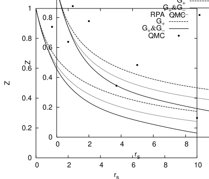
Figure 12: Renormalization constant $Z$ as a function of $r_{s}$ for $0\leq r_{s}\leq 10$. The QMC data have been taken from Ref. conti, .

In Fig. 12 we show our numerical results for the renormalization constant $Z$ in comparison with the QMC data of Ref. conti, . The theory underestimates the value of $Z$ over the whole range of densities explored. Notice that short-range charge-density fluctuations tend to stabilize the normal Fermi liquid, while the simultaneous inclusion of charge- and spin-density fluctuations works in the opposite way.

For the sake of completeness we have collected in Table I a summary of our numerical results for $m^{*}$ and $Z$ at a few values of $r_{s}$. In the next Section we will discuss our results for the QP effective mass in the light of recent experimental results and draw our main conclusions.

V Comparison with experimental results and conclusions

A full analysis of the published data for the effective mass of carriers in Si-MOSFET’s shashkin ; pudalov_prl would require a more complete theoretical study, mainly to account for the two-valley nature of the material. We will focus here instead on the experimental results of Ref. private_zhu, as kindly provided to us by Dr. Zhu prior to publication. At present the data refer to the range $2\lesssim r_{s}\lesssim 6$, so that we cannot judge the performance of the theory in the weak-coupling regime. A quantitative comparison between theory and experiment would also require a refined treatment of a series of effects such as those due to disorder and to finite temperature. We restrict our analysis to the effect of finite sample thickness, by discussing how a softened Coulomb potential modifies $m^{*}$ against the strictly $2D$ results discussed in Sect. IV.2 and shown in Fig. 10. The expectation is that the QP effective mass will be noticeably smaller when a softened Coulomb interaction is at work.

We have thus recalculated $m^{*}$ after renormalizing the bare Coulomb potential by means of a form factor to take into account the finite width of the EG in the GaAs/AlGaAs heterojunction-insulated gate field-effect transistor used in Refs. zhu_2003, and private_zhu, . The appropriate renormalized potential is given by $V_{\bf q}=v_{\bf q}F(qd)/{\bar{\kappa}}$, where

$$F(x)=\left(1+\frac{\kappa_{\rm ins}}{\kappa_{\rm sc}}\right)\frac{8+9x+3x^{2}}{8(1+x)^{3}}+\left(1-\frac{\kappa_{\rm ins}}{\kappa_{\rm sc}}\right)\frac{1}{2(1+x)^{6}}\,,$$ (49)

with $d=[\hbar^{2}\kappa_{\rm sc}/(48\pi m_{z}e^{2}n^{*})]^{1/3}$ representing an effective width of the $2D$ EG ando . Here $\kappa_{\rm ins}=10.9$ and $\kappa_{\rm sc}=12.9$ are the dielectric constants of the insulator and of the space charge layer, ${\bar{\kappa}}$ is their average, $m$ is the band mass in the confinement direction, and $n^{*}=n_{\rm depl}+11n_{\rm\scriptscriptstyle 2D}/32$, the depletion layer charge density $n_{\rm depl}$ being zero in the experiments of Ref. private_zhu, . The results that we obtain with the softened potential are shown in Fig. 13. A caveat to keep in mind is that we have used the same local-field factors as for a zero-thickness $2D$ EG in the lack of a better choice. Thus the results labelled by “$G_{+}$” and “$G_{+}\&G_{-}$” in Fig. 13 contain the effect of finite thickness only through the renormalization of the Coulomb potential. We believe that the explicit dependence of the local fields on the finite width of the $2D$ EG should not change the results of Fig. 13 in a substantial manner.

Comparing the results of Fig. 13 with those in Ref. private_zhu, we can draw the following conclusions: (i) the “$G_{+}$” results, at both the OSA and the Dyson-equation level, do not have the proper functional shape to account for the experimental data; (ii) the RPA and “$G_{+}\&G_{-}$” results are rather similar; and (iii) the “$G_{+}\&G_{-}$” results, which treat charge and spin fluctuations on the same footing, show the best performance against the experimental data. In fact, without the use of any fitting parameters, the “$G_{+}\&G_{-}$” results within the OSA compare in a very reasonable manner with the data. The Dyson-equation results, show instead a relatively small and slowly increasing mass enhancement over the whole range of densities, as discussed for the strictly $2D$ case in Sect. IV.2.

In summary, we have revisited the problem of the microscopic calculation of the quasiparticle self-energy and many-body effective mass enhancement in a $2D$ EG. We have performed a systematic study based on the many-body local-fields theory, taking advantage of the results of the most recent Diffusion Monte Carlo calculations of the static charge and spin response of the EG expressed through static local-field factors. We have carried out extensive calculations of both the real and the imaginary part of the quasiparticle self-energy. We have also presented results for the effective mass enhancement and for the renormalization constant over a wide range of coupling strength. In this respect we have critically examined the merits of the on-shell approximation versus the Dyson-equation calculation. Depending on the local-field factors, the OSA predicts a divergence of the effective mass at strong coupling and a solution of the Dyson equation is necessary in order to obtain a well behaved effective mass. The comparison with the experimental data of Ref. private_zhu, shows that the simultaneous inclusion of charge- and spin-density fluctuations beyond the Random Phase Approximation is crucial in accounting for exchange and short-range correlations, and can lead to substantial corrections at low carrier densities. A possible role of dynamic correlations, entering through the frequency dependence of the local-field factors, remains to be examined.

Appendix A. Details on the explicit calculation of the real part of the CH contribution

Using Eq. (7) we find that the real part of the CH term evaluated at $\omega=\xi_{\bf k}/\hbar$ is given by

$$\left.\Re e\Sigma_{\rm\scriptstyle CH}({\bf k},\omega)\right|_{\omega=\xi_{\bf k}/\hbar}=-\int\frac{d^{2}{\bf q}}{(2\pi)^{2}}\,v_{\bf q}{\mathcal{P}}\int_{0}^{+\infty}\,\frac{d\Omega}{\pi}\,\frac{\Im m[\varepsilon^{-1}({\bf q},\Omega)]}{\xi_{\bf k}/\hbar-\xi_{{\bf k}+{\bf q}}/\hbar-\Omega}\,.$$ (50)

The angular integration can be performed analytically, with the result

$$\int_{0}^{2\pi}\frac{d\theta}{\xi_{\bf k}/\hbar-\xi_{{\bf k}+{\bf q}}/\hbar-\Omega}=\frac{2\pi\,\Theta(\Omega-\Omega_{\rm min}(k))}{\sqrt{[\Omega+\hbar q^{2}/(2m)]^{2}-\hbar^{2}k^{2}q^{2}/m^{2}}}$$ (51)

where $\Omega_{\rm min}(k)=-\hbar q^{2}/(2m)+\hbar kq/m$. In carrying out the frequency integration care must be taken to include the contribution from the plasmon pole $\Omega_{\rm pl}$. Using the expression for the imaginary part of the charge-charge susceptibility near $\Omega_{\rm pl}$,

$$\Im m\chi_{\rm\scriptstyle C}({\bf q},\Omega)=\pi\,v^{-1}_{\rm C}({\bf q})\left.\Re e\chi_{0}({\bf q},\Omega)\right|_{\Omega=\Omega_{\rm pl}}\left[\left.\frac{\partial\Re e\chi_{0}({\bf q},\Omega)}{\partial\Omega}\right|_{\Omega=\Omega_{\rm pl}}\right]^{-1}\delta(\Omega-\Omega_{\rm pl})\,,$$ (52)

we find that the real part of the CH term is given by

$$\left.\Re e\Sigma_{\rm\scriptstyle CH}({\bf k},\omega)\right|_{\omega=\xi_{\bf k}/\hbar}=$$ (53)

$$- \int_{0}^{q_{\rm c}}\frac{qdq}{2\pi}\,\frac{v_{\rm C}({\bf q})\left.\Re e\chi_{0}({\bf q},\Omega)\right|_{\Omega=\Omega_{\rm pl}}}{\sqrt{[\Omega_{\rm pl}+\hbar q^{2}/(2m)]^{2}-\hbar^{2}k^{2}q^{2}/m^{2}}}\,\left[\left.\frac{\partial\Re e\chi_{0}({\bf q},\Omega)}{\partial\Omega}\right|_{\Omega=\Omega_{\rm pl}}\right]^{-1}\Theta(\Omega_{\rm pl}-\Omega_{\rm min}(k))$$

$$- \int_{0}^{+\infty}\frac{qdq}{2\pi}\,{\mathcal{P}}\int_{{\rm max}[0,\Omega_{\rm min}(k),\Omega_{\rm low}]}^{\Omega_{\rm up}}\,\frac{d\Omega}{\pi}\,\frac{v^{2}_{\rm C}({\bf q})\Im m\chi_{\rm\scriptstyle C}({\bf q},\Omega)+3v^{2}_{\rm S}({\bf q})\,\Im m\chi_{\rm\scriptstyle S}({\bf q},\Omega)}{\sqrt{[\Omega+\hbar q^{2}/(2m)]^{2}-\hbar^{2}k^{2}q^{2}/m^{2}}}\,.$$

Here $q_{\rm c}$ marks the onset of Landau damping and $\Omega_{{\rm up}({\rm low})}=\hbar q^{2}/(2m)\pm\hbar qk_{F}/m$ are the upper and lower edges of the electron-hole continuum.

The range of the momentum integration deserves special attention. In the first term in Eq. (53), due to the step function the range of $q$-integration is determined by the intersections between $\Omega_{\rm min}(k)$ and $\Omega_{\rm pl}$ (see Fig. 14). In Sect. IV.1 we have introduced the $r_{s}$-dependent wave number $k_{p}$: this is the wave number $k$ at which $\Omega_{\rm min}(k)$ is tangent to $\Omega_{\rm pl}$. There are two cases: (i) for $k<k_{p}$ there are no intersections and thus the range of $q$-integration goes from $0$ to $q_{c}$; and (ii) for $k\geq k_{p}$ there can be either one ($q_{1}$) or two intersections $(q_{1,2})$, so that the range of integration is $[0,q_{1}]$ or $[0,q_{1}]\cup[q_{2},q_{c}]$, respectively. It is the crossover from condition (i) to (ii) that leads to the plasmon dip in $\left.\Re e\Sigma_{\rm\scriptstyle CH}({\bf k},\omega)\right|_{\omega=\xi_{\bf k}/\hbar}$.

In the second term in Eq. (53) the range of $q$-integration runs up to $q=+\infty$ and this gives rise to the logarithmic divergence mentioned in Ref. footnote, . As already discussed in Sect. II, what matters are self-energy differences, which are free of singularities. Numerically we deal only with the finite quantity $\left.\Re e\Sigma_{\rm\scriptstyle CH}({\bf k},\omega)\right|_{\omega=\xi_{\bf k}/\hbar}-\Sigma_{\rm\scriptstyle CH}(k_{F},0)$.

Appendix B. “Line+residue” decomposition

In this Appendix we discuss a mathematically equivalent decomposition of the QP self-energy, first introduced by Quinn and Ferrell quinn , which has been often employed in the literature mahan . This amounts to writing

$$\Sigma_{\rm\scriptstyle ret}({\bf k},\omega)=\Sigma_{\rm X}({\bf k})+\Sigma_{\rm\scriptstyle line}({\bf k},\omega)+\Sigma_{\rm\scriptstyle res}({\bf k},\omega)\,.$$ (54)

Here the first term is the Hartree-Fock self-energy stern_1973

$$\Sigma_{\rm X}({\bf k})=\left\{\begin{array}[]{l}-2e^{2}k_{F}\,{\rm E}(\bar{k}^{2})/\pi\,\hskip 142.26378pt\mbox{$(\bar{k}\leq 1)$}\\ -2e^{2}k_{F}\,\bar{k}\,[{\rm E}(1/\bar{k}^{2})-(1-1/\bar{k}^{2})\,{\rm K}(1/\bar{k}^{2})]/\pi\,\hskip 4.26773pt\mbox{$(\bar{k}>1)$}\end{array}\right.$$ (55)

where $\bar{k}=k/k_{F}$ and ${\rm K}(x)$, ${\rm E}(x)$ are complete elliptical integrals of the first and second kind, respectively. The second term in Eq. (54), which is purely real, is given by

$$\Sigma_{\rm\scriptstyle line}({\bf k},\omega)=-\int\frac{d^{2}{\bf q}}{(2\pi)^{2}}v_{\bf q}\int_{-\infty}^{\infty}\frac{d\Omega}{2\pi}\left[\frac{1}{\varepsilon({\bf q},i\Omega)}-1\right]\,\frac{1}{\omega+i\Omega-\xi_{{\bf k}+{\bf q}}/\hbar}\,.$$ (56)

Finally, the third term is the so-called “residue” contribution,

$$\Sigma_{\rm\scriptstyle res}({\bf k},\omega)=\int\frac{d^{2}{\bf q}}{(2\pi)^{2}}v_{\bf q}\left[\frac{1}{\varepsilon({\bf q},\omega-\xi_{{\bf k}+{\bf q}}/\hbar)}-1\right]\,\left[\Theta(\omega-\xi_{{\bf k}+{\bf q}}/\hbar)-\Theta(-\xi_{{\bf k}+{\bf q}}/\hbar)\right]\,.$$ (57)

Within this decomposition it is the “line” contribution which needs to be regularized for a ultraviolet divergence.

As a check of our numerical results obtained by means of the SX-CH decompositions, we have recalculated the QP self-energy, effective mass, and renormalization constant by this alternative route. This turned out to require a substantially harder numerical effort. For completeness we summarize in Figs. 15 and 16 our results for the “line” and “residue” terms.

Figure 6: The real part of the SX contribution to the retarded self-energy (in units of Ryd) evaluated at $\omega=\xi_{\bf k}/\hbar$, as a function of $k/k_{F}$ for $r_{s}=1$ (top panel) and $5$ (bottom panel).

Figure 7: The real part of the CH contribution to the retarded self-energy (in units of Ryd) evaluated at $\omega=\xi_{\bf k}/\hbar$, as a function of $k/k_{F}$ for $r_{s}=1$ (top panel) and $5$ (bottom panel).

Figure 8: The real part of the retarded self-energy (in units of Ryd) evaluated at $\omega=\xi_{\bf k}/\hbar$, as a function of $k/k_{F}$ for $r_{s}=1$ and $5$. $\mu_{\rm QMC}$ is the chemical potential from the QMC ground-state energy.

Figure 9: The absolute value of the imaginary part of the retarded self-energy (in units of Ryd) evaluated at $\omega=\xi_{\bf k}/\hbar$, as a function of $k/k_{F}$ for $r_{s}=1$ (top panel) and $5$ (bottom panel).

Figure 10: Effective mass enhancement as a function of $r_{s}$ for $0\leq r_{s}\leq 10$. The inset shows an enlargement of the results for $r_{s}\leq 1$. The lines show the results from Eq. (46), while the symbols (except for the dots) are from Eq. (48). The QMC data (dots) are from Ref. kwon_1994, .

Figure 11: Illustrating the divergence of the effective mass within the OSA. The three curves starting from unity at $r_{s}=0$ refer to the quantity $1+(m/\hbar^{2}k_{F})\partial_{k}\Re e\Sigma^{\rm R}_{\rm\scriptstyle ret}(k_{F},0)$, and the other three curves to $\hbar^{-1}|\partial_{\omega}\Re e\Sigma^{\rm R}_{\rm\scriptstyle ret}(k_{F},0)|$. The intersection of two lines with the same line-style in the two sets of curves corresponds to a zero in the denominator of Eq. (48) and thus to a divergence in $m^{*}_{\rm OSA}$. The inset shows this divergence occurring within the RPA at $r_{s}\simeq 15.5$.

Figure 13: Effective mass enhancement for a quasi-$2D$ EG confined in a GaAs/AlGaAs triangular quantum well of the type used in Refs. zhu_2003, and private_zhu, . The notation is as in Fig. 10.

Figure 14: Illustrating the integration range relevant to Eq. (53), with $\Omega$ in units of $\varepsilon_{F}/\hbar$. The shaded area represents the electron-hole continuum. $\Omega_{\rm min}(q)$ is shown for three values of $k$ (dashed curves): from top to bottom, $k=3.0k_{F},k_{p}$, and $0.8k_{F}$ with $k_{p}\simeq 2.32k_{F}$. The plasmon dispersion relation $\Omega_{\rm pl}(q)$ (dotted curve) is also shown.

Figure 15: The exchange plus regularized “line” contribution to the retarded self-energy (in units of Ryd) evaluated at $\omega=\xi_{\bf k}/\hbar$, as a function of $k/k_{F}$ for $r_{s}=1$ and $5$.

Figure 16: The real part of the “residue” contribution to the retarded self-energy (in units of Ryd) evaluated at $\omega=\xi_{\bf k}/\hbar$, as a function of $k/k_{F}$ for $r_{s}=1$ (top panel) and $5$ (bottom panel).

Table 1: QP effective mass and renormalization constant of a paramagnetic $2D$ EG. The arrows refer to the divergence in the OSA as explained in the main text.

$r_{s}$	Various calculations	$m^{*}_{\rm D}/m$	$m^{*}_{\rm OSA}/m$	$Z$
1	RPA	1.022	1.033	0.670
	$G_{+}$	0.972	0.961	0.710
	$G_{+}\&G_{-}$	1.026	1.040	0.658
2	RPA	1.082	1.168	0.526
	$G_{+}$	1.004	1.007	0.585
	$G_{+}\&G_{-}$	1.144	1.349	0.486
3	RPA	1.121	1.322	0.444
	$G_{+}$	1.030	1.061	0.510
	$G_{+}\&G_{-}$	1.247	2.026	0.391
5	RPA	1.167	1.696	0.349
	$G_{+}$	1.066	1.172	0.419
	$G_{+}\&G_{-}$	1.410	$\nearrow$	0.289
10	RPA	1.215	3.650	0.244
	$G_{+}$	1.100	1.415	0.311
	$G_{+}\&G_{-}$	1.834	$\nearrow$	0.166

References

- (1) D.M. Ceperley, Nature 397, 386 (1999).
- (2) K. S. Singwi and M.P. Tosi, in Solid State Physics 36, ed. H. Ehrenreich, F. Seitz and D. Turnbull (Academic, New York, 1981), p. 177.
- (3) N.H. March, Electron Correlation in the Solid State (Imperial College Press, London, 1999).
- (4) E.P. Wigner, Phys. Rev. 46, 1002 (1934).
- (5) D.M. Ceperley and B.J. Alder, Phys. Rev. Lett. 45, 566 (1980); B.J. Alder, D.M. Ceperley, and E.L. Pollock, Int. J. Quant. Chem. 16, 49 (1982).
- (6) B. Tanatar and D.M. Ceperley, Phys. Rev. B 39, 5005 (1989).
- (7) S. Moroni, D.M. Ceperley, and G. Senatore, Phys. Rev. Lett. 69, 1837 (1992).
- (8) Y. Kwon, D.M. Ceperley, and R.M. Martin, Phys. Rev. B 50, 1684 (1994).
- (9) S. Moroni, D.M. Ceperley and G. Senatore, Phys. Rev. Lett. 75, 689 (1995).
- (10) F. Rapisarda and G. Senatore, Austr. J. Phys. 49, 161 (1996).
- (11) G. Ortiz, M. Harris, and P. Ballone, Phys. Rev. Lett. 82, 5317 (1999).
- (12) G. Senatore, S. Moroni, and D.M. Ceperley, in Quantum Monte Carlo Methods in Physics and Chemistry, edited by M.P. Nightingale and C.J. Umrigar (Kluwer, Dordrecht, 1999).
- (13) D. Varsano, S. Moroni, and G. Senatore, Europhys. Lett. 53, 348 (2001).
- (14) F.H. Zong, C. Lin, and D.M. Ceperley, Phys. Rev. E 66, 036703 (2002).
- (15) C. Attaccalite, S. Moroni, P. Gori-Giorgi, and G. Bachelet, Phys. Rev. Lett. 88, 256601 (2002).
- (16) L.D. Landau, Sov. Phys. JEPT, 3, 920 (1957).
- (17) J.J. Quinn and R.A. Ferrell, Phys. Rev. 112, 812 (1958).
- (18) T.M. Rice, Ann. Phys. (NY) 31, 100 (1965).
- (19) J. Hubbard, Proc. Roy. Soc. A 240, 739 (1957) and 243, 336 (1957).
- (20) C.S. Ting, T.K. Lee, and J.J. Quinn, Phys. Rev. Lett. 34, 870 (1975); see also T.K. Lee, C.S. Ting, and J.J. Quinn, Solid State Commun. 16, 1309 (1975).
- (21) G. Vignale and K.S. Singwi, Phys. Rev. B 32, 2156 (1985).
- (22) X. Zhu and A.W. Overhauser, Phys. Rev. B 33, 925 (1986).
- (23) S. Yarlagadda and G.F. Giuliani, Solid State Commun. 69, 677 (1989).
- (24) C.A. Kukkonen and A.W. Overhauser, Phys. Rev. B 20, 550 (1979).
- (25) D.R. Hamann and A.W. Overhauser, Phys. Rev. 143, 183 (1966).
- (26) S. Rahman and G. Vignale, Phys. Rev. B 30, 6951 (1984).
- (27) G.E. Santoro and G.F. Giuliani, Phys. Rev. B 39, 12818 (1989); S. Yarlagadda and G.F. Giuliani, ibid. 40, 5432 (1989).
- (28) T.K. Ng and K.S. Singwi, Phys. Rev. B 34, 7738 and 7743 (1986).
- (29) S. Yarlagadda and G.F. Giuliani, Phys. Rev. B 49, 7887 (1994) and 61, 12556 (2000).
- (30) S. Yarlagadda and G. F. Giuliani, Phys. Rev. B 49, 14188 (1994).
- (31) B. Davoudi, M. Polini, G.F. Giuliani, and M.P. Tosi, Phys. Rev. B 64, 153101 and 233110 (2001).
- (32) T. Ando, A.B. Fowler, and F. Stern, Rev. Mod. Phys. 54, 437 (1982).
- (33) A.A. Abrikosov, Fundamentals of the Theory of Metals (North Holland, Amsterdam, 1988); E.M. Lifshitz and L.P. Pitaevskii, Physical Kinetics (Nauka, Moscow, 1979).
- (34) J.L. Smith and P.J. Stiles, Phys. Rev. Lett. 29, 102 (1972).
- (35) G. Abstreiter, J.P. Koothaus, J.F. Koch, and G. Dorda, Phys. Rev. B 14, 2480 (1976).
- (36) F.F. Fang and P.J. Stiles, Phys. Rev. 174, 823 (1968).
- (37) T. Neugebauer, K. von Klitzing, G. Landwehr, and G. Dorda, Solid State Commun. 17, 295 (1975).
- (38) For a review on the MIT see e.g. E. Abrahams, S.V. Kravchenko, and M.P. Sarachik, Rev. Mod. Phys. 73, 251 (2001); B.L. Altshuler, D.L. Maslov, and V.M. Pudalov, Physica E 9, 209 (2001).
- (39) V.T. Dolgopolov, G.V. Kravchenko, A.A. Shashkin, and S.V. Kravchenko, JEPT Lett. 55, 733 (1992); D. Simonian, S.V. Kravchenko, M.P. Sarachik, and V.M. Pudalov, Phys. Rev. Lett. 79, 2304 (1997); V.M. Pudalov, G. Brunthaler, A. Prinz, and G. Bauer, JEPT Lett. 65, 932 (1997).
- (40) T. Okamoto, K. Hosoya, S. Kawaji, and A. Yagi, Phys. Rev. Lett. 82, 3875 (1999).
- (41) S.A. Vitkalov, H. Zheng, K.M. Mertes, M.P. Sarachik, and T.M. Klapwijk, Phys. Rev. Lett. 87, 086401 (2001).
- (42) A.A. Shashkin, S.V. Kravchenko, V.T. Dolgopolov, and T.M. Klapwijk, Phys. Rev. Lett. 87, 086801 (2001) and Phys. Rev. B 66, 073303 (2002).
- (43) V.M. Pudalov, M.E. Gershenson, H. Kojima, N. Butch, E.M. Dizhur, G. Brunthaler, A. Prinz, and G. Bauer, Phys. Rev. Lett. 88, 196404 (2002); see also V.M. Pudalov, M.E. Gershenson, and H. Kojima, cond-mat/0110160.
- (44) E. Tutuc, S. Melinte, and M. Shayegan, Phys. Rev. Lett. 88, 036805 (2002).
- (45) H. Noh, M.P. Lilly, D.C. Tsui, J.A. Simmons, E.H. Hwang, S. Das Sarma, L.N. Pfeiffer, and K.W. West, Phys. Rev. B 68, 165308 (2003).
- (46) J. Zhu, H.L. Stormer, L.N. Pfeiffer, K.W. Baldwin, and K.W. West, Phys. Rev. Lett. 90, 056805 (2003).
- (47) K. Vakili, Y.P. Shkolnikov, E. Tutuc, E.P. De Poortere, and M. Shayegan, cond-mat/0403191.
- (48) I.M. Lifshitz and A.M. Kosevich, Sov. Phys. JEPT 2, 636 (1956); J.M. Luttinger, Phys. Rev. 121, 1251 (1961); Yu.A. Bychkov and L.P. Gor’kov, Sov. Phys. JEPT 14, 1132 (1962).
- (49) K. Miyake and C.M. Varma, Solid State Commun. 85, 335 (1993); S. Curnoe and P.C.E. Stamp, Phys. Rev. Lett. 80, 3312 (1998).
- (50) G.W. Martin, D.L. Maslov, and M.Yu. Reizer, Phys. Rev. B 68, 241309 (2003).
- (51) J. Zhu et al., private communication.
- (52) F. Stern, Phys. Rev. Lett. 18, 546 (1967).
- (53) F. Stern, Phys. Rev. Lett. 30, 278 (1973).
- (54) H.M. Böhm, S. Conti, and M.P. Tosi, J. Phys.: Condens. Matter 8, 781 (1996); S. Conti, R. Nifosì, and M.P. Tosi, ibid. 9, L475 (1997); R. Nifosì, S. Conti, and M.P. Tosi, Phys. Rev. B 58, 12758 (1998); G. Vignale and W. Kohn, in Electronic Density Functional Theory, Recent Progress and New Directions, edited by J. Dobson, G. Vignale, and M.P. Das (Plenum, New York, 1998) p. 199; Z. Qian and G. Vignale, Phys. Rev. B 65, 235121 (2002) and 68, 195113 (2003).
- (55) P. Noziéres, Theory of Interacting Fermi Systems (Benjamin, New York, 1964).
- (56) L. Hedin, Phys. Rev. 139, A796 (1965).
- (57) G.D. Mahan and B.E. Sernelius, Phys. Rev. Lett. 62, 2718 (1989).
- (58) A. Holas, in Strongly Coupled Plasma Physics, eds. F.J. Rogers and H.E. DeWitt, (Plenum, New York, 1986), p. 463; G.E. Santoro and G.F. Giuliani, Phys. Rev. B 37, 4813 (1988); G. Vignale, Phys. Rev. B 38, 6445 (1988).
- (59) The leading term in the large- behavior of the static local-field factors in Eq. (42) induces a logarithmic ultraviolet divergence in the real part of , as can be demonstrated through a power-counting argument. Such a divergence is not surprising, because the theory that we are using applies only in a shell of momenta close to the Fermi momentum (see Sect. II.2), and it cancels out in the QP excitation energy since this quantity depends only on self-energy differences. Obviously, to determine the chemical potential one has to make recourse to a different approach: for instance, can be obtained from parametrizations of the QMC ground-state energy rapisarda ; attaccalite or calculated by refined theories of the ground-state energy (see e.g. R. Asgari, B. Davoudi, and M.P. Tosi, Solid State Commun. (in press) for the EG).
- (60) Y. Isawa and H. Yasuhara, Solid State Commun. 46, 807 (1983); S. Nagano, K.S. Singwi, and S. Ohnishi, Phys. Rev. B 29, 1209 (1984) and 31, 3166 (1985); R. Asgari, M. Polini, B. Davoudi, and M.P. Tosi, Solid State Commun. 125, 139 (2003).
- (61) G.F. Giuliani and J.J. Quinn, Phys. Rev. B 26, 4421 (1982).
- (62) R. Asgari, B. Davoudi, and B. Tanatar, Solid State Commun. 130, 13 (2004).
- (63) S. Conti, Ph. D. Thesis, Scuola Normale Superiore (Pisa, 1997).
- (64) G.D. Mahan, Many-particle Physics (Plenum, New York, 1990), Chapts. 3 and 5.