Spectrum of an open disordered quasi-two-dimensional electron system:
strong orbital effect of the weak in-plane magnetic field

Abstract

The effect of an in-plane magnetic field upon open quasi-two-dimensional electron and hole systems is investigated in terms of the carrier ground-state spectrum. The magnetic field, classified as weak from the viewpoint of correlation between size parameters of classical electron motion and the gate potential spatial profile is shown to efficiently cut off extended modes from the spectrum and to change singularly the mode density of states (MDOS). The reduction in the number of current-carrying modes, right up to zero in magnetic fields of moderate strength, can be viewed as the cause of magnetic-field-driven metal-to-insulator transition widely observed in two-dimensional systems. Both the mode number reduction and the MDOS singularity appear to be most pronounced in the mode states dephasing associated with their scattering by quenched-disorder potential. This sort of dephasing is proven to dominate the dephasing which involves solely the magnetic field whatever level of the disorder.

I Introduction

The apparent metallic state widely observed in two-dimensional (2D) systems of Si MOSFET type as well as in GaAs/AlGaAs heterostructures bib:AbKrSar01 ; bib:KrSar04 obviously contradicts the well-known one-parameter scaling theory bib:AALR79 and as yet has not received generally accepted theoretical explanation. The existence of such a state is mostly believed to result from Coulomb interaction of carriers, which is rather strong in the systems of low electron and hole density. Estimations of this interaction indeed can cause the surmise that just this interaction should lead to quite strong dephasing effect upon electrons which otherwise would be localized due to scattering by the disorder potential, thus residing in coherent states. However, at the present time the lack of a comprehensive theory for Coulomb interaction in solids precludes from making certain conclusions about its predominant role in forming the metallic ground state of 2D electron systems. In particular, a considerable challenge in this connection is presented by commonplace observations of the dephasing time saturation in different systems, including 2D ones, at temperatures very close to zero (see, e. g., Ref. bib:LB02, and numerous references therein).

Besides the unexpected conduction state of quench-disordered 2D systems, the metal-insulator transition (MIT) is normally observed there, which currently has not been proven unambiguously to be determined exclusively by the level of the disorder. No less puzzling is also the abnormally large response of 2D electron and hole systems to the relatively weak in-plane magnetic field, bib:DKSK92 which is known to significantly suppress the metallic behaviour of the carriers and even to drive the system into the insulating regime. bib:SKSP97 ; bib:MZVSK01 ; bib:SKK01 ; bib:GMRPW02

In so far as the electrons confined to move in a narrow near-surface potential well are weakly coupled to the in-plane magnetic field through their orbital degree of freedom, it is widely believed that such a field promotes localization of carriers, and thus the MIT, mainly due to strong spin-related effects. bib:SHPLRRSG98 ; bib:OHKY99 ; bib:Metal99 The relatively rare papers where orbital coupling was analyzed by taking into account the finite width of potential wells forming real two-dimensional systems are not rated by now as fully convincing. Specifically, the relatively simple model suggested in Ref. bib:DSHw00, do not exhibit sufficiently abrupt transition between metallic and dielectric regimes, whereas in Ref. bib:MFA02, only corrections caused by weak localization of carriers are studied, which can hardly serve as the conclusive proof for the physical mechanism of the observed effects.

Previously in Refs. bib:Tar00, ,bib:Tar03, , one-particle theory capable of explaining the metallic ground state as well as MIT in disordered 2D systems not subjected to magnetic field was developed starting from basic positions essentially different from those of scaling theories. Specifically, the conductance of a strictly 2D bib:Tar00 and a quasi-2D bib:Tar03 system was calculated in terms of quantum states pertinent to a perfect finite-size open system of waveguide geometry. In this approach, the metallic value of the conductance is bound up with the primary existence of coherent extended waveguide modes rather than one-particle electronic states originally localized by the disorder. Energy levels of these collective mode states can be widened by quenched disorder provided that scattering is ensured between extended modes having different longitudinal energies. This type of scattering can be viewed (mathematically) as inelastic, although it is physically provided by a static random potential. In the suggested approach, all extended modes other than the particular one, if any, can be regarded as the dephasing bath. With gradual strengthening of the disorder, the conductance transforms from its ballistic value in a perfect system, which equals the number of extended modes times the conductance quantum, to the diffusive value coincident with standard Drude conductance if the system possesses the number of extended modes noticeably greater than unity.

In the present work, we apply the mode approach of Refs. bib:Tar00, ; bib:Tar03, to examine the influence of the in-plane magnetic field upon spectrum of the electrons restricted to move in a planar, yet three-dimensional, open quantum well. It will be shown that at large values of the transverse aspect ratio of such an electron waveguide even a rather weak magnetic field can significantly affect the electron spectrum. This appears in considerable magnetic-field responsivity of the number of extended modes, the latter being normally identified as conducting channels, as well as in MDOS sensitivity to the magnetic field. The former factor is well known to control the value of the ballistic conductance of the confined current carriers whereas the latter (MDOS) governs substantially the mode states dephasing associated with scattering of the electrons by the disorder potential. Interestingly, mode entanglement solely due to the magnetic field, with no disorder whatsoever, leads to electron mass renormalization and does not affect the width of the energy levels of the collective electron states.

II The model

Two-dimensional electron and hole systems in practical applications can be modelled, in view of their open property in the direction of current flow, as planar quantum waveguides whose transverse structure is governed by lateral (depletion) potential. The exact form of the confining potential well is of minor importance for its principal application which reduces to the restriction of electron transport in the direction normal to the interfacial area and, consequently, to the “transverse” quantization of the electron spectrum. In this study, we assume the open quasi-two-dimensional (Q2D) system of carriers having the form of three-dimensional “electron waveguide” of rectangular cross-section, which occupies the coordinate region

$$x\in(-L/2,L/2)\ ,$$

$$y\in[-W/2,W/2]\ ,$$ (1)

$$z\in[-H/2,H/2]\ ,$$

as shown in Figure 1. The length $L$, the width $W$ as well as the

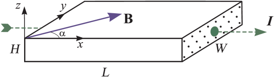
Figure 1: The geometry of Q2D electron waveguide subject to in-plane magnetic field $\mathbf{B}$.

height $H$ of the model system will be regarded as arbitrary except that the thickness $H$ will be assumed to serve as a small length parameter which will be specified below. The electron system will be thought of as open at the ends $x=\pm L/2$ and closed by infinite-wall potentials at all lateral boundaries. The magnetic field $\mathbf{B}$ is taken to point parallel to $x$-$y$ plane at arbitrary angle with respect to $x$-axes.

Since main transport coefficients, in particular the conductance, are expressed in terms of one-particle propagators of carriers, we will analyze the equation for the retarded Green function of Fermi particles with energy $\varepsilon_{F}=k_{F}^{2}$. In the Fermi-liquid approximation it has the form

$$\left[\left(\nabla-\frac{2\pi i}{\Phi_{0}}\mathbf{A}(\mathbf{r})\right)^{2}+k_{F}^{2}+i0-V(\mathbf{r})\right]G(\mathbf{r},\mathbf{r}^{\prime})\\ =\delta(\mathbf{r}-\mathbf{r}^{\prime})\ ,$$ (2)

where $\Phi_{0}=hc/e$ is the magnetic flux quantum, $\mathbf{A}(\mathbf{r})$ is the vector potential of the external magnetic field, $V(\mathbf{r})$ is the scalar random potential due to, say, impurities or rough boundaries of the confining potential well. We adopt hereinafter the system of units with $\hbar=2m=1$, $m$ denoting the electron effective mass.

With the magnetic field gauged so as $\mathbf{A}(\mathbf{r})=(B_{y}z,-B_{x}z,0)$, the equation (2) takes the form

$$\Bigg{[}\nabla^{2}+k_{F}^{2}+i0-V(\mathbf{r})-\frac{4\pi i}{\Phi_{0}}\left(B_{y}z\frac{\partial}{\partial x}-B_{x}z\frac{\partial}{\partial y}\right)\\ -\left(\frac{2\pi}{\Phi_{0}}\right)^{2}\mathbf{B}^{2}z^{2}\Bigg{]}G(\mathbf{r},\mathbf{r}^{\prime})=\delta(\mathbf{r}-\mathbf{r}^{\prime})\ .$$ (3)

At this stage it is expedient to go over from the initially three-dimensional problem to a set of strictly one-dimensional problems, individual for each of the modes. Towards this end, as a first step one should carry out Fourier transformation of equation (3) over the transverse radius-vector $\mathbf{r}_{\perp}=(y,z)$. The appropriate set of eigenfunctions has the form

$$\bm{|}\mathbf{r}_{\perp};\bm{\mu}\bm{\rangle}=\frac{2}{\sqrt{WH}}\sin\left[\left(\frac{y}{W}+\frac{1}{2}\right)\pi n\right]\\ \times\sin\left[\left(\frac{z}{H}+\frac{1}{2}\right)\pi m\right]\ ,$$ (4)

where $\bm{\mu}=(n,m)$, with $n,m\in\mathbb{N}$, is the vector mode index conjugate to the coordinate vector $\mathbf{r}_{\perp}$. With functions (4), equation (3) is readily transformed to the set of coupled equations for mode Fourier components of the function $G(\mathbf{r},\mathbf{r}^{\prime})$, viz.

$$\left[\frac{\partial^{2}}{\partial x^{2}}+k^{2}_{\bm{\mu}}+i0-{\mathcal{V}}_{\bm{\mu}}(x)\right]G_{\bm{\mu}\bm{\mu}^{\prime}}(x,x^{\prime})\\ -\sum_{\bm{\nu}\neq\bm{\mu}}\hat{{\mathcal{U}}}_{\bm{\mu}\bm{\nu}}(x)G_{\bm{\nu}\bm{\mu}^{\prime}}(x,x^{\prime})=\delta_{\bm{\mu}\bm{\mu}^{\prime}}\delta(x-x^{\prime})\ .$$ (5)

Here,

$$k^{2}_{\bm{\mu}}=k^{2}_{F}-\left(\frac{\pi n}{W}\right)^{2}-\left(\frac{\pi m}{H}\right)^{2}$$ (6)

is the unperturbed mode energy,

$${\mathcal{V}}_{\bm{\mu}}(x)=V_{\bm{\mu}\bm{\mu}}(x)+\frac{H^{2}}{12l_{B}^{4}}\left(1-\frac{6}{\pi^{2}m^{2}}\right)$$ (7)

is the diagonal-in-mode-indices matrix element of the total potential which includes the impurity part $V(\mathbf{r})$ and both of the magnetic terms in square brackets of equation (3), $l_{B}=\sqrt{\Phi_{0}/2\pi|\mathbf{B}|}$ is the magnetic length. The term $V_{\bm{\mu}\bm{\mu}}(x)$ in Eq. (7) is the diagonal element of the mode matrix $\|V_{\bm{\mu}\bm{\nu}}\|$ whose components are evaluated as

$$V_{\bm{\mu}\bm{\nu}}(x)=\int_{S}\textit{d}\,\mathbf{r}_{\perp}\bm{\langle}\mathbf{r}_{\perp};\bm{\mu}\bm{|}V(\mathbf{r})\bm{|}\mathbf{r}_{\perp};\bm{\nu}\bm{\rangle}\ ,$$ (8)

integration is over cross-section $S$ of the quantum well. Off-diagonal mode matrix elements $\hat{{\mathcal{U}}}_{\bm{\mu}\bm{\nu}}(x)$ in Eq. (5) also include both the disorder and the magnetic-field originated potentials, viz.

$$\hat{{\mathcal{U}}}_{\bm{\mu}\bm{\nu}}(x)=V_{\bm{\mu}\bm{\nu}}(x)+2iH\left(\frac{S_{\bm{\mu}\bm{\nu}}^{(x)}}{l_{x}^{2}W}-\frac{S_{\bm{\mu}\bm{\nu}}^{(y)}}{l_{y}^{2}}\frac{\partial}{\partial x}\right)+C_{\bm{\mu}\bm{\nu}}\frac{H^{2}}{l_{B}^{4}}\ .$$ (9)

In Eq. (9), $\ l_{i}\$ is the partial magnetic length given by $l_{i}^{2}=\nolinebreak\Phi_{0}/2\pi|B_{i}|$, numerical coefficients, which are specifical for the geometry of the quantum well, have the form

$$\begin{aligned} S_{\bm{\mu}\bm{\nu}}^{(x)}=&\varsigma_{x}\frac{4nn_{1}}{n^{2}-n_{1}^{2}}\sin^{2}\left[\frac{\pi}{2}(n-n_{1})\right]\big{(}1-\delta_{mm_{1}}\big{)}\\ &\times\frac{8mm_{1}}{\pi^{2}(m^{2}-m_{1}^{2})^{2}}\sin^{2}\left[\frac{\pi}{2}(m-m_{1})\right]\ ,\end{aligned}$$ (10a)

$$\begin{aligned} S_{\bm{\mu}\bm{\nu}}^{(y)}=&\varsigma_{y}\delta_{nn_{1}}\big{(}1-\delta_{mm_{1}}\big{)}\\ &\times\frac{8mm_{1}}{\pi^{2}(m^{2}-m_{1}^{2})^{2}}\sin^{2}\left[\frac{\pi}{2}(m-m_{1})\right]\ ,\end{aligned}$$ (10b)

$$\begin{aligned} C_{\bm{\mu}\bm{\nu}}=&\delta_{nn_{1}}\big{(}1-\delta_{mm_{1}}\big{)}\\ &\times\frac{8mm_{1}}{\pi^{2}(m^{2}-m_{1}^{2})^{2}}\cos^{2}\left[\frac{\pi}{2}(m-m_{1})\right]\ ,\end{aligned}$$ (10c)

with $\varsigma_{i}=B_{i}/|B_{i}|=\mathrm{\,sgn\,}B_{i}$. In expressions (10), mode indices are designated such that $\bm{\mu}=(n,m)$ and $\bm{\nu}=\nolinebreak(n_{1},m_{1})$.

The potentials ${\mathcal{V}}_{\bm{\mu}}(x)$ and $\hat{{\mathcal{U}}}_{\bm{\mu}\bm{\nu}}(x)$ in Eq. (5) may be thought of as responsible for coherent intra-mode and incoherent inter-mode scattering, respectively. We thus adopt in this work the approach where interactions of the electron system with both the impurities and the magnetic field are exploited on equal footing, that is they are treated as the problems of scattering by additive static potentials which are basically different in correlation properties only.

III Reduction to one-dimensional dynamic problems

A set of equations (5), though describing mode propagation in one spatial dimension, cannot certainly be regarded as a really one-dimensional dynamical problem by virtue of strong correlation of different modes via inter-mode potentials (9). Formally, this manifests itself in co-existence in (5) of purely intra-mode propagators, i. e. the Green functions having identical mode indices, and inter-mode propagators $G_{\bm{\nu}\bm{\mu}}(x,x^{\prime})$ with $\bm{\nu}\neq\bm{\mu}$.

One can obviate these complications using the method suggested in Refs. bib:Tar00, ; bib:Tar03, . In the above papers, non-diagonal elements of the mode matrix $\|G_{\bm{\mu}\bm{\mu}^{\prime}}\|$ were proven to be expressed, by means of some linear operation, through the respective diagonal elements only. Substitution of thus represented inter-mode propagators into Eq. (5) results in the following set of strictly one-dimensional equations for intra-mode propagators $G_{\bm{\mu}\bm{\mu}}(x,x^{\prime})$,

$$\left[\frac{\partial^{2}}{\partial x^{2}}+k^{2}_{\bm{\mu}}+i0-{\mathcal{V}}_{\bm{\mu}}(x)-\hat{\mathcal{T}}_{\bm{\mu}}\right]G_{\bm{\mu}\bm{\mu}}(x,x^{\prime})=\delta(x-x^{\prime})\ ,$$

$$\quad\text{for}\ \forall\bm{\mu}\ .$$ (11)

Here, $\hat{\mathcal{T}}_{\bm{\mu}}$ is the operator (integral) potential, well-known as the $T$-matrix in the quantum theory of scattering,bib:Newton68 ; bib:Taylor72 which acts in the $x$-coordinate space $\mathbb{X}$. It has the form

$$\hat{\mathcal{T}}_{\bm{\mu}}=\bm{P}_{\bm{\mu}}\hat{\mathcal{U}}(\openone-\hat{\mathsf{R}})^{-1}\hat{\mathsf{R}}\bm{P}_{\bm{\mu}}\ ,$$ (12)

where $\hat{\mathcal{U}}$ and $\hat{\mathsf{R}}$ are the operators acting in the mixed mode-coordinate space ${\mathsf{\overline{M}}_{\bm{\mu}}}$ constructed as a direct product of the space $\mathbb{X}$ and the truncated mode space which incorporates the whole set of mode indices except the unique mode index $\bm{\mu}$. The operator $\hat{\mathcal{U}}$ is specified in ${\mathsf{\overline{M}}_{\bm{\mu}}}$ by its matrix elements

$$\bm{\langle}x,\bm{\nu}\bm{|}\hat{\mathcal{U}}\bm{|}x^{\prime},\bm{\nu^{\prime}}\bm{\rangle}={\mathcal{U}}_{\bm{\nu}\bm{\nu^{\prime}}}(x)\delta(x-x^{\prime})\ ,$$ (13)

matrix elements of the operator $\hat{\mathsf{R}}$ have the form

$$\bm{\langle}x,\bm{\nu}\bm{|}\hat{\mathsf{R}}\bm{|}x^{\prime},\bm{\nu^{\prime}}\bm{\rangle}=G^{(V)}_{\bm{\nu}}(x,x^{\prime})\hat{{\mathcal{U}}}_{\bm{\nu}\bm{\nu^{\prime}}}(x^{\prime})\ .$$ (14)

The function $G^{(V)}_{\bm{\nu}}(x,x^{\prime})$ in (14) will be thought of as the trial mode Green function which satisfies the equation resulting from Eq. (5) provided that all inter-mode potentials are put identically equal to zero,

$$\left[\frac{\partial^{2}}{\partial x^{2}}+k^{2}_{\bm{\mu}}+i0-{\mathcal{V}}_{\bm{\mu}}(x)\right]G^{(V)}_{\bm{\mu}}(x,x^{\prime})=\delta(x-x^{\prime})\ .$$ (15)

The operator $\bm{P}_{\bm{\mu}}$ in (12) is the projection operator whose action reduces to assigning the given value $\bm{\mu}$ to the nearest mode index of an arbitrary operator standing next to it (either to the left or right), without affecting the product in the $\mathbb{X}$ space.

With intra-mode Green functions found from the set of equations (11), all inter-mode propagators are expressed via the operator relation

$$\hat{G}_{\bm{\nu}\bm{\mu}}=\bm{P}_{\bm{\nu}}(\openone-\hat{\mathsf{R}})^{-1}\hat{\mathsf{R}}\bm{P}_{\bm{\mu}}\hat{G}_{\bm{\mu}\bm{\mu}}\ ,$$ (16)

$\hat{G}_{\bm{\nu}\bm{\mu}}$ and $\hat{G}_{\bm{\mu}\bm{\mu}}$ being thought of as matrices in $\mathbb{X}$-space. The initially three-dimensional problem thus reduces to the set of separate 1D equations (11), each representing the closed problem provided that trial Green functions are independently found from equation (15).

To analyze the mode states spectrum, i. e. the spectrum of differential operator in Eq. (11), it is worthwhile to renormalize mode energies in Eqs. (11) and (15) by extracting from the initial mode energy (6) the non-random “magnetic” part of the intra-mode potential ${\mathcal{V}}_{\bm{\mu}}(x)$, thus defining the new “unperturbed” mode energy

$$\varkappa_{\bm{\mu}}^{2}=k^{2}_{\bm{\mu}}-\frac{H^{2}}{12l_{B}^{4}}\left(1-\frac{6}{\pi^{2}m^{2}}\right)\ .$$ (17)

In such a way one is led to solve, in place of equations (11) and (15), a couple of different, though equivalent, equations, namely

$$\begin{aligned} \left[\frac{\partial^{2}}{\partial x^{2}}+\varkappa^{2}_{\bm{\mu}}+i0-V_{\bm{\mu}\bm{\mu}}(x)-\hat{\mathcal{T}}_{\bm{\mu}}\right]G&{}_{\bm{\mu}\bm{\mu}}(x,x^{\prime})\\ &=\delta(x-x^{\prime})\end{aligned}$$ (18a)

and

$$\left[\frac{\partial^{2}}{\partial x^{2}}+\varkappa^{2}_{\bm{\mu}}+i0-V_{\bm{\mu}\bm{\mu}}(x)\right]G^{(V)}_{\bm{\mu}}(x,x^{\prime})=\delta(x-x^{\prime})\ ,$$ (18b)

which must be supplied with correct boundary conditions at open ends of the system, to be discussed in the next section.

IV Spectrum of the mode states

To examine differential operator (18a), which is of principal import for our purpose, one should first solve Eq. (18b) for the truly one-dimensional trial Green function. In the absence of magnetic field, this problem was resolved in Ref. bib:Tar00, where arbitrary statistical moments of the function $G^{(V)}_{\bm{\mu}}(x,x^{\prime})$ were found in the case of open system subject to weak disorder potential by applying the averaging technique appropriate for causal-type random functionals. The condition for weak impurity scattering (WIS), which we assume to hold in this study as well, can be cast to the form of the inequality pair

$$k^{-1}_{F},\,r_{c}\ll\ell\ ,$$ (19)

were $r_{c}$ is the correlation radius of the random potential, $\ell$ is the electron mean free path relating to it.

In the case of non-zero magnetic field the solution to Eq. (18b) is much more involved than that accomplished in Ref. bib:Tar00, . This will be thoroughly examined in a separate publication, while here we outline the solution along with criteria of its applicability.

Given the magnetic potentials, to adequately take into account the open property of one-dimensional system governed by equation (18b) one should explore this equation on the extended $x$-axis rather than on disordered and subject to magnetic field interval $\mathcal{L}=\nolinebreak(-L/2,L/2)$. Being considered on the whole axis, equation (18b) describes the motion of a quantum particle created with energy $k^{2}_{\bm{\mu}}$ at point $x^{\prime}$ and then propagating in two-component scalar potential with bounded support. The regular component of this combined potential is due to the magnetic field. It has the form $V^{(reg)}(x)=\nolinebreak\theta(L/2-\nolinebreak|x|)\frac{H^{2}}{12l_{B}^{4}}\left(1-\frac{6}{\pi^{2}m^{2}}\right)$, whereas the random component, which is of impurity origin, is covered by the function $V^{(ran)}(x)=\theta(L/2-\nolinebreak|x|)V_{\bm{\mu}\bm{\mu}}(x)$.

To perform configurational averaging over the random part of the potential it is worthwhile to express the trial Green function in terms of wave functions of causal type rather than functions that meet the initially stated boundary-value (BV) problem. This may be achieved by employing the formula (for the sake of clarity we omit mode index $\bm{\mu}$)

$$G^{(V)}(x,x^{\prime})=\frac{1}{\mathcal{W}}\big{[}\psi_{+} (x)\psi_{-}(x^{\prime})\theta(x-x^{\prime})$$

$$+\psi_{+}(x^{\prime})\psi_{-}(x)\theta(x^{\prime}-x)\big{]}\ ,$$ (20)

where $\psi_{\pm}(x)$ are two different solutions of homogeneous equation (15) with boundary conditions specified for each of them at only one end of the system, viz. $x\to\pm\infty$, depending on the sign index, $\mathcal{W}$ is the Wronskian of those solutions. With this representation, the trial propagator itself meets, as it must, the initial BV problem.

The openness of the finite-size system under consideration implies that far from the source coordinate $x^{\prime}$, specifically at $x\to\pm\infty$, Green function $G^{(V)}(x,x^{\prime})$ must have the form of outgoing free waves. In view of boundedness of the support of the potentials, at large values of $|x|$ functions $\psi_{\pm}(x)$ have to be taken as

$$\psi_{\pm}(x)=c_{\pm}\exp\big{[}\pm ik(x-L/2)\big{]}\ .$$ (21)

Inside the magnetically biased interval $\mathcal{L}$, in order to properly take into account the electron backscattering from the potential $V^{(ran)}(x)$, it is worthwhile to seek wave functions $\psi_{\pm}(x)$ in the form

$$\psi_{\pm}(x)=\pi_{\pm}(x)\mathrm{e}^{i\varkappa(\pm x-L/2)}-i\gamma_{\pm}(x)\mathrm{e}^{-i\varkappa(\pm x-L/2)}\ ,$$ (22)

with $\varkappa^{2}$ specified in (17). Under WIS conditions (19), envelope functions $\pi_{\pm}(x)$ and $\gamma_{\pm}(x)$ in (22) can be regarded as smooth factors in comparison with near-standing fast exponentials, which leads to the following coupled dynamic equations,

$$\pm\pi^{\prime}_{\pm}(x)+i\eta(x)\pi_{\pm}(x)+\zeta^{*}_{\pm}(x)\gamma_{\pm}(x)=0\ ,$$ (23a)

$$\pm\gamma^{\prime}_{\pm}(x)-i\eta(x)\gamma_{\pm}(x)+\zeta_{\pm}(x)\pi_{\pm}(x)=0\ .$$ (23b)

Random functions $\eta(x)$ and $\zeta_{\pm}(x)$ in Eqs. (23) are constructed as normalized packets of spatial harmonics of the impurity potential  $V(x)\equiv V_{\bm{\mu}\bm{\mu}}(x)$, which have the form

$$\eta(x)=\frac{1}{2\varkappa}\int_{x-l}^{x+l}\frac{\mathrm{d}t}{2l}V(t)\ ,$$ (24a)

$$\zeta_{\pm}(x)=\frac{1}{2\varkappa}\int_{x-l}^{x+l}\frac{\mathrm{d}t}{2l}V(t)\exp[2i\varkappa(\pm x-L/2)]\ .$$ (24b)

Spatial averaging in (24) is carried out over the interval $2l$ of arbitrary length intermediate between small lengths $\varkappa^{-1}$ and $r_{c}$, on the one hand, and the large scattering length (to be determined self-consistently), on the other. In view of these limitations, the “potentials” $\eta(x)$ and $\zeta_{\pm}(x)$ provide forward and backward scattering of harmonics $\pm\varkappa$, respectively.

By joining the solutions (22) and (21) at the end points of the interval $\mathcal{L}$ we arrive at the exact boundary conditions for the envelopes $\pi_{\pm}(x)$ and $\gamma_{\pm}(x)$, viz.

$$\pi_{\pm}(\pm L/2)= \mathrm{const}\ ,$$ (25a)

$$\gamma_{\pm}(\pm L/2)= \mathcal{R}^{(B)}\pi_{\pm}(\pm L/2)\ .$$ (25b)

The quantity

$$\mathcal{R}^{(B)}=-i\frac{k-\varkappa}{k+\varkappa}\ ,$$ (26)

as it follows from (22), is the amplitude reflection coefficient from the boundary between magnetically biased and unbiased regions. This reflection will be hereinafter referred to as “magnetic scattering” associated with the above introduced potential $V^{(reg)}(x)$.

Below in this paper, scattering associated with both of the potentials, $V^{(ran)}(x)$ and $V^{(reg)}(x)$, will be regarded as weak. The weakness of the impurity scattering implies the inequalities (19) whereas the magnetic scattering will be thought of as weak provided that the requirement is met $|\mathcal{R}^{(B)}|\ll 1$. From (25b) and (17) one can make sure that in terms of appropriate physical parameters the condition for weak magnetic scattering (WMS) may be expressed as the inequality

$$\left(\frac{H}{R_{c}}\right)^{2}\ll 1\ ,$$ (27)

where $R_{c}=k_{F}l_{B}^{2}$ is the maximal classical cyclotron radius of the electron orbit. It is just from the viewpoint of this constraint that we will regard the in-plane magnetic field to be weak.

As far as the impurity scattering is concerned, to do the averaging over realizations of the potential $V(\mathbf{r})$ this random function will be thought of to possess the following correlation properties,

$$\big{<}V(\mathbf{r})\big{>} =0\ ,$$ (28a)

$$\big{<}V(\mathbf{r})V(\mathbf{r}^{\prime})\big{>} =\mathcal{QW}(x-x^{\prime})\delta(\mathbf{r}_{\perp}-\mathbf{r}^{\prime}_{\perp})\ ,$$ (28b)

angular brackets denote configurational averaging. Under WIS conditions (19), the equalities (28) are sufficient to adequately accomplish the averaging for rather wide class of the random potential statistics, since in this case function $V(\mathbf{r})$ may be regarded as approximately Gaussian distributed.bib:LGP82

By applying the averaging technique outlined in the Appendix the average trial Green function is obtained in the following form, which is valid provided WIS and WMS conditions hold simultaneously,

$$\left<G^{(V)}_{\bm{\mu}}(x,x^{\prime})\right>\approx\frac{-i}{2\varkappa_{\bm{\mu}}}\exp\left\{\left[i\varkappa_{\bm{\mu}}-\frac{1}{2}\left(\frac{1}{L_{f}^{(V)}(\bm{\mu})}+\frac{1}{L_{b}^{(V)}(\bm{\mu})}\right)\right]|x-x^{\prime}|\right\}\ .$$ (29)

Here,

$$L_{f}^{(V)}(\bm{\mu})=\left(\frac{4}{3}\right)^{2}\frac{S}{\mathcal{Q}}\varkappa^{2}$$ (30a)

and

$$L_{b}^{(V)}(\bm{\mu})=\frac{L_{f}^{(V)}(\bm{\mu})}{\widetilde{\mathcal{W}}(2\varkappa_{\bm{\mu}})}$$ (30b)

are the extinction lengths related to forward ($f$) and backward ($b$) scattering by the potential $V_{\bm{\mu}\bm{\mu}}(x)$, $\widetilde{\mathcal{W}}(q)$ is the Fourier transform of function $\mathcal{W}(x)$ from (28b). With the result (29), the average square norm of the operator $\hat{\mathsf{R}}$ from (12) can be represented as a sum of “impurity” and “magnetic” terms, viz. $\big{<}\|\hat{\mathsf{R}}\|^{2}\big{>}\approx\big{<}\|\hat{\mathsf{R}}^{(imp)}\|^{2}\big{>}+\big{<}\|\hat{\mathsf{R}}^{(B)}\|^{2}\big{>}$, which are estimated as

$$\big{<}\|\hat{\mathsf{R}}^{(imp)}\|^{2}\big{>}\sim\frac{1}{k_{F}\ell}\ll 1\ ,$$ (31a)

$$\big{<}\|\hat{\mathsf{R}}^{(B)}\|^{2}\big{>}\sim\left(\frac{H}{R_{c}}\right)^{2}\ll 1\ .$$ (31b)

Inequalities (31) permit simplification of the operator potential $\hat{\mathcal{T}}_{\bm{\mu}}$ since the inverse operator in (12) can be approximately replaced with the unit operator. The inter-mode potential thus reduces to the relatively simple form,

$$\hat{\mathcal{T}}_{\bm{\mu}}\approx\bm{P}_{\bm{\mu}}\hat{\mathcal{U}}\hat{\mathcal{G}}^{(V)}\hat{\mathcal{U}}\bm{P}_{\bm{\mu}}\ ,$$ (32)

where $\hat{\mathcal{G}}^{(V)}$ stands for the operator in ${\mathsf{\overline{M}}_{\bm{\mu}}}$ which is specified by the matrix elements of the following form,

$$\bm{\langle}x,\bm{\nu}\bm{|}\hat{\mathcal{G}}^{(V)}\bm{|}x^{\prime},\bm{\nu}^{\prime}\bm{\rangle}=G^{(V)}_{\bm{\nu}}(x,x^{\prime})\delta_{\bm{\nu}\bm{\nu}^{\prime}}\ .$$ (33)

Unlike quasi-local intra-mode potential $V_{\bm{\mu}\bm{\mu}}(x)$, the operator potential (32) possesses, even in the absence of magnetic field, the nonzero mean value. Therefore, to apply further a perturbation theory it is reasonable to represent this operator as a sum of averaged and fluctuating parts, i. e. $\hat{\mathcal{T}}_{\bm{\mu}}=\big{<}\hat{\mathcal{T}}_{\bm{\mu}}\big{>}+\nolinebreak\Delta\hat{\mathcal{T}}_{\bm{\mu}}$. With regard to Eq. (9), the mean operator $\big{<}\hat{\mathcal{T}}_{\bm{\mu}}\big{>}$ can be splitted (though quite conventionally) into the local “impurity” and essentially non-local “magnetic” terms. The action of short-correlated impurity part of this operator reduces to multiplication of the mode propagator by the complex self-energy factor,bib:Tar00 ; bib:Tar03

$$\Big{[}\big{<}\hat{\mathcal{T}}^{(imp)}_{\bm{\mu}}\big{>}G_{\bm{\mu}\bm{\mu}}\Big{]}(x,x^{\prime})=-\varSigma^{(imp)}_{\bm{\mu}}G_{\bm{\mu}\bm{\mu}}(x,x^{\prime})\ ,$$ (34)

where $\varSigma^{(imp)}_{\bm{\mu}}=\Delta\varkappa_{\bm{\mu}}^{2}+i/\tau_{\bm{\mu}}^{(\varphi)}$ and the notations are used

$$\Delta\varkappa_{\bm{\mu}}^{2} =\frac{\mathcal{Q}}{S}\sum_{\bm{\nu}\neq\bm{\mu}}\mathcal{P}\int_{-\infty}^{\infty}\frac{\mathrm{d}q}{2\pi}\;\frac{\widetilde{\mathcal{W}}(q+\varkappa_{\bm{\mu}})}{q^{2}-\varkappa_{\bm{\nu}}^{2}}\ ,$$ (35a)

$$\frac{1}{\tau_{\bm{\mu}}^{(\varphi)}} =\frac{\mathcal{Q}}{4S}\overline{\sum_{\bm{\nu}\neq\bm{\mu}}}\frac{1}{\varkappa_{\bm{\nu}}}\left[\widetilde{\mathcal{W}}(\varkappa_{\bm{\mu}}-\varkappa_{\bm{\nu}})+\widetilde{\mathcal{W}}(\varkappa_{\bm{\mu}}+\varkappa_{\bm{\nu}})\right]\ .$$ (35b)

Symbol $\mathcal{P}$ in (35a) stands for the integral principal value, the bar over the summation index in (35b) signifies that the summation is carried out over extended modes only. The conditional character of the term “impurity self energy” with reference to $\varSigma^{(imp)}_{\bm{\mu}}$ is related to the mere fact that this factor is actually determined by both the impurity potential, whose correlator is proportional to the factor of $\mathcal{Q}$, and the magnetic field, which renormalizes the wavenumbers $\varkappa_{\bm{\mu},\bm{\nu}}$ and also adjusts the number of extended modes, see next subsection.

The action of the expressly non-local “magnetic” part of the operator $\big{<}\hat{\mathcal{T}}_{\bm{\mu}}\big{>}$ is specified by the formula

$$\big{[}\big{<}\hat{\mathcal{T}}_{\bm{\mu}}^{(B)}\big{>}G_{\bm{\mu}\bm{\mu}}\big{]}(x,x^{\prime}) = \sum_{\bm{\nu}\neq\bm{\mu}}\left[2iH\left(\frac{S_{\bm{\mu}\bm{\nu}}^{(x)}}{Wl_{x}^{2}}-\frac{S_{\bm{\mu}\bm{\nu}}^{(y)}}{l_{y}^{2}}\frac{\partial}{\partial x}\right)+C_{\bm{\mu}\bm{\nu}}\frac{H^{2}}{l_{B}^{4}}\right]$$ (36)

$$\times\int_{L}\textit{d}x_{1}\left<G^{(V)}_{\bm{\nu}}(x,x_{1})\right>\left[2iH\left(\frac{S_{\bm{\bm{\nu}\mu}}^{(x)}}{Wl_{x}^{2}}-\frac{S_{\bm{\nu}\bm{\mu}}^{(y)}}{l_{y}^{2}}\frac{\partial}{\partial x_{1}}\right)+C_{\bm{\nu}\bm{\mu}}\frac{H^{2}}{l_{B}^{4}}\right]G_{\bm{\mu}\bm{\mu}}(x_{1},x^{\prime})\ ,$$

wherefrom the “magnetic” self-energy, which is applicable under WS conditions, is immediately deduced

$$\varSigma^{(B)}_{\bm{\mu}}=-4H^{2}\sum_{\bm{\nu}\neq\bm{\mu}}\frac{\left(\frac{S_{\bm{\mu}\bm{\nu}}^{(x)}}{Wl_{x}^{2}}-i\varkappa_{\bm{\mu}}\frac{S_{\bm{\mu}\bm{\nu}}^{(y)}}{l_{y}^{2}}\right)\left(\frac{S_{\bm{\nu}\bm{\mu}}^{(x)}}{Wl_{x}^{2}}-i\varkappa_{\bm{\mu}}\frac{S_{\bm{\nu}\bm{\mu}}^{(y)}}{l_{y}^{2}}\right)}{\varkappa_{\bm{\mu}}^{2}-\varkappa_{\bm{\nu}}^{2}-i\varkappa_{\bm{\nu}}\left(\frac{1}{L_{f}^{(V)}(\bm{\nu})}+\frac{1}{L_{b}^{(V)}(\bm{\nu})}\right)}\ .$$ (37)

IV.1 Mode content of the open quantum system

Both the impurity and the magnetic self-energies are complex-valued quantities, whose real parts renormalize mode energies whereas the imaginary parts determine the uncertainty of energy levels. The requirement for mode energies to be positive defined specifies the number of extended modes in the quantum system, which is normally referred to as the number of conducting channels, $N_{c}$. Computation of exact number of these modes, though clear in principle, is an intricate problem in general. For the system under consideration the number $N_{c}$ can be most easily found in the particular case of the magnetic field oriented lengthwise with respect to the current direction, i. e. for $\mathbf{B}\parallel Ox$. In this case mode energy renormalization due to the inter-mode magnetic scattering, which is covered by the magnetic self-energy (37), is small as compared with the intra-mode magnetic correction present in the mode energy (17). Taking account of this fact, one can calculate the number of extended modes as

$$N_{c}=\sum_{m=1}^{N_{c}^{(z)}}N_{c}^{(y)}(m)\ ,\vspace{-.3cm}$$ (38a)

where

$$N_{c}^{(z)}=\mathrm{int}\left[\frac{k_{F}H}{\pi}\sqrt{1-\frac{H^{2}}{12R_{c}^{2}}}\right]\vspace{-.1cm}$$ (38b)

is the number of quantization levels in $$z$$-direction, whose energies lie beneath the Fermi energy, and

$$N_{c}^{(y)}(m)=\mathrm{int}\left[\frac{k_{F}W}{\pi}\sqrt{1-\left(\frac{\pi m}{k_{F}H}\right)^{2}-\frac{H^{2}}{12R_{c}^{2}}\left(1-\frac{6}{\pi^{2}m^{2}}\right)}\right]$$ (38c)

is the number of $y$-directional quantization levels pertinent to the $m$-th level of $z$-quantization. Symbol $\mathrm{int[\ldots]}$ in (38b) and (38c) denotes the integer part of the number enclosed in square brackets.

The sum (38a) can be readily evaluated in the case where the number of extended modes relating to both of the transverse axes of the quantum waveguide is large as compared to unity. By replacing the sum with the integral one readily gets

$$N_{c}\approx\frac{k_{F}^{2}S}{4\pi}\left(1-\frac{H^{2}}{12R_{c}^{2}}\right)\ ,$$ (39)

wherefrom it is evident that application of the in-plane magnetic field can significantly reduce the number of extended modes, even though inequality (27) holds true. This reduction is definitely the geometrical effect which is due to the curving of the electron orbits in the magnetic field, and thus it can be only taken into consideration within the model of a finite-width quantum well that forms a 2D system.

In Fig. 2, the numerical results for the number of effective conducting channels as a function of the inverse magnetic field scaled

1em

Figure 2: The magnetic-field dependence of the number of effective conducting channels. The parameter $\nu$ is the Landau filling factor, $\nu=(k_{F}l_{B})^{2}$.

as the Landau filling factor $\nu=\nolinebreak(k_{F}l_{B})^{2}=\nolinebreak k_{F}R_{c}$ are presented. The collapse of the number of current-carrying modes with a growth in the magnetic field is apparent, regardless of the quantum waveguide thickness $H$, the width $W$ is assumed constant. The in-plane rotation of the magnetic field smoothly changes the presented picture because the real part of self-energy (37) can at most reach the same (on the order of magnitude) value as the intra-mode magnetic addend in (17).rem1

In Fig. 3, the relation between the number of channels and the effective thickness of the quantum waveguide is presented, which actually demonstrates the dependence of $N_{c}$ on the depletion voltage adjusting the width of the near-surface potential well. In the extremely low magnetic field (black curve) the number of channels increases nearly linear with growing $H$, in accordance with standard geometrical consideration applicable to systems of waveguide configuration, and also with the conventional Ohm’s law which is undoubtedly valid for bulk conductors. With the growing magnetic field, the

1em

Figure 3: The number of conducting channels vs the width of the near-surface potential well at different values of the Landau filling factor. The shaded area below the dashed curve covers the parameter region where the criterion (27) is violated.

conventional geometric increase in the number of channels gets slower, gradually indicating the trend for lowering the number of conducting modes. This unusual dependence of the mode content of the electron waveguide on its effective thickness is due to non-monotonic dependence on $H$ of the mode energy (17).

Obviously, on a further increase of the magnetic field the tendency towards lowering the number of conducting channels must be stabilized owing to terms $\propto l_{B}^{-4}$ in square brackets in r.h.s. of Eq. (36). However, this can happen only in the domain of relatively strong magnetic fields, where the WMS condition is violated and the approximate expression (32) for the inter-mode potential is no longer applicable. In such magnetic fields, the bulk quantum Hall effect is expected to come in the foreground, which is beyond the scope of this paper.

IV.2 Dephasing of the mode states: the magnetic-field driven disorder

Besides the impact on the number of extended quantum modes whose transverse energies are beneath the Fermi level, the in-plane magnetic field can significantly affect the coherent properties of the conducting channels. This field controls the imaginary parts of both the impurity-governed self-energy (35) and the magnetic self-energy (37). Both of these self-energies arise due to the inter-mode scattering. One should bear in mind, however, that $\varSigma^{(imp)}_{\bm{\mu}}$ is basically determined by scattering from the impurity potential whereas the magnetic self-energy, $\varSigma^{(B)}_{\bm{\mu}}$, originates in the main from mode mixing due to the orbital effect of in-plane magnetic field.

It is important to note that intermixing of channels which is controlled solely by the magnetic field cannot result in significant dephasing of mode states. By comparing the imaginary part of self-energy (37) and the level width (35b) one can determine that the ratio of “purely magnetic” and “impurity-governed” dephasing rates is evaluated as

$$\frac{\Im\varSigma^{(B)}_{\bm{\mu}}}{\Im\varSigma^{(imp)}_{\bm{\mu}}}\sim\left[\frac{H}{R_{c}k_{F}W}\left(\frac{B_{x}}{B}\right)^{2}+\frac{H}{R_{c}}\left(\frac{B_{y}}{B}\right)^{2}\right]^{2}\ll 1\ .$$ (40)

This implies that under WMS condition the magnetic-field originated dephasing is negligible, whatever strength of the disorder. The conclusion is thus unavoidable that strong inter-mode mixing resulting from the magnetic field cannot give rise to significantly widening the mode levels unless there exists some random potential due to, say, impurities or the roughness of quantum well boundaries, which can mediate the dephasing effect of the magnetic field. The specific role of the magnetic field, as far as the mode entanglement is concerned, reduces to the change in collective parameters of the electron motion, such as the mode content of the confined system and the mode density of states, and in such an indirect way to modification of scattering parameters pertinent to random generators of inter-mode transitions (i. e., the impurity scattering cross-section, the polar pattern of electron reflection from rough boundaries, etc.).

The influence of the magnetic field upon transport parameters manifests itself directly through the mode dephasing rate. Analytically, the estimate of this quantity can be most easily deduced from Eq. (35b) in the case where the number of quantization levels related to both of the transverse directions is large as compared to unity and the sum in Eq. (35b) can be replaced with the integral. The dephasing rate for the particular mode $\bm{\mu}$ in this case reads

$$\frac{1}{\tau_{\bm{\mu}}^{(\varphi)}(B)}\approx\frac{1}{\tau_{\bm{\mu}}^{(\varphi)}(0)}\sqrt{1-\frac{H^{2}}{12R_{c}^{2}}}\ ,$$ (41)

where $1/\tau_{\bm{\mu}}^{(\varphi)}(0)=k_{F}\mathcal{Q}/4\pi$ is the $\bm{\mu}$-th mode level width attributed to scattering due to the disorder potential only, with no external magnetic field.bib:Tar03 The value of this zero-field level width equals exactly half the inverse mean free time calculated within the framework of classical kinetic theory. Note that in the domain of weak magnetic fields corresponding to inequality (27) the dephasing rate (41) decreases nearly quadratically in the magnetic field and has universal value, the same for each of the extended modes.bib:Tar03

The result (41), which is actually semiclassical, is of limited applicability. Upon varying the magnetic field the number of extended modes changes stepwise. Therefore the majority of physical quantities are bound to exhibit the oscillatory behaviour, which is closely related to well-known van Hove singularities in MDOS. In Fig. 4, the dephasing rates obtained numerically from Eq. (35b) for two specific modes of

1em

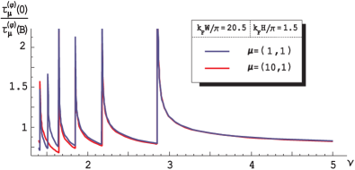
Figure 4: The dephasing rate (35b) for two particular modes vs inverse magnetic field.

the electron waveguide are shown as functions of the inverse magnetic field. Square-root singularities manifestly develop on both of the curves. One can also notice that scattering frequencies for different modes start to noticeably deviate from one another only in the range of relatively strong magnetic fields, where the number of extended modes assumes the value comparable with unity.

Besides the magnetic-field singularities depicted in Fig. 4, in Fig. 5 the dephasing rate of the particular mode vs size parameters of the quantum waveguide is presented for two distinct values of $|\mathbf{B}|$. Here, MDOS oscillations caused by abrupt changes in the number of conducting channels also make themselves very evident.

1em

Figure 5: The dephasing rate vs the quantum waveguide thickness at different strengths of in-plane magnetic field. The broken fraction of the lower curve falls into the range of parameters where WMS condition (27) is violated.

We are led to conclude that by means of the orbital coupling to the electrons in a Q2D conducting system the in-plane magnetic field can take an effect which in some sense is analogous to that of electrostatic confinement potential. At the same time, in contrast to the magnetic-field-controlled singularities of the dephasing rate, which are depicted in Fig. 4, oscillations of truly geometrical origin are noticeably more complicated. The distinction is caused by substantially different response of the effective mode energy (17) to the magnetic field, on the one hand, and to size parameters of the confined electron system, on the other. However, it should be noted that in both of the graphs, 4 and 5, the reduction of the dephasing by quenched disorder is clearly visible as the magnetic field grows. This fact can serve as the indication of increasing coherence of electron transport in quench-disordered Q2D systems if they are subjected to external magnetic field.

V Conclusion

In this study we have demonstrated that the observed giant positive magnetoresistance of 2D electron and hole systems subject to parallel magnetic field can be reasonably explained in the framework of Fermi liquid theory being applied to structures created by confining potential wells of finite rather than zero width. The magnetic field coupling to the carrier orbital motion which is due to finite thickness of quasi-two-dimensional layers, even though rather weak from semi-classical point of view, has been proven to influence quite essentially the collective electron spectrum. The reduction in the number of extended modes with a growth of the magnetic field, as seen from Fig. 2, is very significant, continuing right up to zero in moderately strong fields, whereas individual electron trajectories in the plane normal to the magnetic field can go far beyond the effective thickness of the gated carrier system. The mode truncation effect of the in-plane magnetic field is the more noticeable the larger is the aspect ratio of the confining potential well forming the electron waveguide.

Since the number of extended modes, according to the Landauer theory, specifies the conductance of a bounded system, the results presented in Figs. 2 and 3 can be directly related to the experiment. In fact, they may be regarded as showing the conductance dependence on the corresponding parameters in the case of a perfect confining potential well. As the perfect we mean a waveguide-type structure in which any mechanism of collective scattering of properly defined carrier modes does not exist. This actually implies that no scattering fields other than those involved in the unperturbed quasi-particle state formation in a particular system are taken into account. Specifically, the collective states pertinent to the problem considered in this study are specified by the confining potential profile. In the absence of the disorder potential the collective electron motion should be regarded as ballistic, even though individual carriers do experience strong (specular) scattering at side boundaries of the potential well.

If some random potential is involved, e. g., impurities or the roughness of quantum well boundaries, it should lead to stochastic rather than regular scattering of the primordial quasi-particles. It seems advantageous to separate this type of scattering into two kinds, namely, intra- and inter-mode scattering. The former type of scattering provides renormalization of transport parameters and also gives rise to Anderson localization of carrier states in the direction of current. The latter type, inelastic in form from the viewpoint of mode theory, leads to stochastic spreading of mode energy levels, or, in other words, to spatial dephasing of mode states. At first glance, it may appear that inter-mode scattering caused exclusively by the magnetic field is bound to produce the dephasing effect analogous to that introduced by the quenched disorder. However, the estimate (40) is obviously contradicting to this expectation. According to the evaluation, in the absence of random potential, which ensures probabilistic property of mode energy levels, no imaginary part must be contained in the mode self-energy, in spite of substantial inter-mode mixing due to the magnetic field.

Physically, this fact seems to be quite natural. Indeed, if one chooses to model lateral confinement of a Q2D carrier system by the quadratic rather than the rectangular potential, eigen-functions of the transverse Hamiltonian could be obviously selected so as to completely avoid the mode coupling due to the magnetic field. The additional random potential, though static, would be in this case the only cause of the mode levels widening. At the same time, the quadratic confinement possesses the same symmetry of the confined system as the rectangular well does. Therefore, it would be difficult to substantiate the drastic difference of the results obtained within the framework of these two models if one is guided by general considerations only.

Fortunately, the result (40) reveals the lack (in the asymptotic sense) of the magnetic-field-originated dephasing of the natural carrier spectrum. Certainly, the magnetic field does take part in the mode level spreading, yet mostly through the dependence on this field of the number of extended modes and of the mode density of states. This parameters essentially determine the impurity-originated dephasing rate (35b), which can thus be viewed as being produced by the magnetic-field-dependent disorder. The idea of the “magnetic-field-driven disorder” was previously suggested in Ref. bib:PBPB01, , so the result (35b) can be viewed as substantiating the rationality of such an interpretation. Clearly, in order to make a detailed comparison with experimental observations it is necessary to derive required formulas for the magnetocondactance. This work will be postponed for the next publication.

*

Appendix A Disorder averaging of the trial Green function

After substitution of functions (22) into (20), the trial Green function inside magnetically biased interval $\mathcal{L}$ can be represented as a sum of four packets of spatial harmonics, viz.

$$G^{(V)}(x,x^{\prime})=\mathcal{G}_{1}(x,x^{\prime})\mathrm{e}^{i\varkappa(x-x^{\prime})}+\mathcal{G}_{2}(x,x^{\prime})\mathrm{e}^{-i\varkappa(x-x^{\prime})}+\mathcal{G}_{3}(x,x^{\prime})\mathrm{e}^{i\varkappa(x+x^{\prime})}+\mathcal{G}_{4}(x,x^{\prime})\mathrm{e}^{-i\varkappa(x+x^{\prime})}\ .$$ (42)

Here, smooth envelope functions are given as

$$\mathcal{G}_{1}(x,x^{\prime})=\frac{-i}{2\varkappa}\mathcal{A}(x)\left[\Theta_{+}\frac{\pi_{-}(x^{\prime})}{\pi_{-}(x)}-\Theta_{-}\frac{\gamma_{+}(x^{\prime})}{\pi_{+}(x)}\Gamma_{-}(x)\mathrm{e}^{2i\varkappa L}\right]\ ,$$ (43a)

$$\mathcal{G}_{2}(x,x^{\prime})=\frac{-i}{2\varkappa}\mathcal{A}(x)\left[\Theta_{-}\frac{\pi_{+}(x^{\prime})}{\pi_{+}(x)}-\Theta_{+}\Gamma_{+}(x)\frac{\gamma_{-}(x^{\prime})}{\pi_{-}(x)}\mathrm{e}^{2i\varkappa L}\right]\ ,$$ (43b)

$$\mathcal{G}_{3}(x,x^{\prime})=\frac{-1}{2\varkappa}\mathcal{A}(x)\mathrm{e}^{i\varkappa L}\left[\Theta_{+}\frac{\gamma_{-}(x^{\prime})}{\pi_{-}(x)}+\Theta_{-}\frac{\pi_{+}(x^{\prime})}{\pi_{+}(x)}\Gamma_{-}(x)\right]\ ,$$ (43c)

$$\mathcal{G}_{4}(x,x^{\prime})=\frac{-1}{2\varkappa}\mathcal{A}(x)\mathrm{e}^{i\varkappa L}\left[\Theta_{-}\frac{\gamma_{+}(x^{\prime})}{\pi_{+}(x)}+\Theta_{+}\Gamma_{+}(x)\frac{\pi_{-}(x^{\prime})}{\pi_{-}(x)}\right]\ ,$$ (43d)

where the notations are used

$$\mathcal{A}(x)=\left[1+\Gamma_{+}(x)\Gamma_{-}(x)\mathrm{e}^{2i\varkappa L}\right]^{-1}\ ,$$ (44a)

$$\Gamma_{\pm}(x)=\gamma_{\pm}(x)/\pi_{\pm}(x)\ ,$$ (44b)

$$\Theta_{\pm}=\theta[\pm(x-x^{\prime})]\ .$$ (44c)

As regards the functions $\Gamma_{\pm}(x)$, their physical meaning is readily deduced from Eq. (22). They represent reflection factors of spatial harmonics $\pm\varkappa$ incident at the point $x$ onto the layers with end coordinates $x$ and $\pm L/2$, respectively. This factors meet the Riccati-type dynamic equations,

$$\pm\frac{\mathrm{d}\Gamma_{\pm}(x)}{\mathrm{d}x}=2i\eta(x)\Gamma_{\pm}(x)-\zeta_{\pm}(x)+\zeta_{\pm}^{*}(x)\Gamma_{\pm}^{2}(x)\ ,$$ (45)

with boundary conditions stemming from (25),

$$\Gamma_{\pm}(\pm L/2)=\mathcal{R}^{(B)}\ .$$ (46)

The averaging technique for the functionals of random fields (24) was elaborated in Refs. bib:Tar00, ; bib:MakTar01, ; bib:FreiTar01, . Here we only briefly indicate the main peculiarities of dealing with functionals of such a sort and present the result of the function (42) averaging.

Having regard to correlation relations (28) it was proven bib:Tar00 ; bib:MakTar01 ; bib:FreiTar01 that binary correlation functions of the effective random fields (24) under WIS conditions can be cast to the form

$$\big{<}\eta(x)\eta(x^{\prime})\big{>}=\frac{1}{L_{f}^{(V)}}F_{l}(x-x^{\prime})\ ,$$ (47a)

$$\big{<}\zeta_{\pm}(x)\zeta_{\pm}^{*}(x^{\prime})\big{>}=\frac{1}{L_{b}^{(V)}}F_{l}(x-x^{\prime})\ ,$$ (47b)

where $L_{f}$ and $L_{b}$ are the forward and the backward scattering lengths given in (30) for the particular mode $\bm{\mu}$. The function $F_{l}(x)$ has the form

$$F_{l}(x)=\int_{-\infty}^{\infty}\frac{\mathrm{d}q}{2\pi}\mathrm{e}^{iqx}\frac{\sin^{2}(ql)}{(ql)^{2}}=\frac{1}{2l}\left(1-\frac{|x|}{2l}\right)\theta(2l-|x|)$$ (48)

and plays the role of under-limiting $\delta$-function when averaging smooth factors similar to the envelopes (43). Before averaging the function (42) it makes sense to go over from functions $\gamma_{\pm}(x)$, $\pi_{\pm}(x)$ and $\zeta_{\pm}(x)$ to phase-renormalized functions

$$\widetilde{\gamma}_{\pm}(x) =\gamma_{\pm}(x)\exp\left[\pm i\int_{x}^{\pm L/2}\mathrm{d}x_{1}\eta(x_{1})\right]\ ,$$ (49a)

$$\widetilde{\pi}_{\pm}(x) =\pi_{\pm}(x)\exp\left[\mp i\int_{x}^{\pm L/2}\mathrm{d}x_{1}\eta(x_{1})\right]\ ,$$ (49b)

$$\widetilde{\zeta}_{\pm}(x) =\zeta_{\pm}(x)\exp\left[\pm 2i\int_{x}^{\pm L/2}\mathrm{d}x_{1}\eta(x_{1})\right]\ ,$$ (49c)

which enables one to remove the forward-scattering random field $\eta(x)$ from all dynamic equations and to separate it out in the form of exponential factors. In particular, note then that correlation relation (47b) remains unchanged after renormalization (49c).

One can easily reveal that in view of short-range correlation of random functions (24) and due to the causal nature of functionals being averaged, the averaging of functionals with different sign indices in (43) can be done separately. By averaging the equation

$$\pm\frac{\mathrm{d}\widetilde{\Gamma}_{\pm}(x)}{\mathrm{d}x}=-\widetilde{\zeta}_{\pm}(x)+\widetilde{\zeta}_{\pm}^{*}(x)\widetilde{\Gamma}_{\pm}^{2}(x)$$ (50)

using the Furutsu-Novikov formula for gaussian random process bib:Klyats86 we obtain

$$\langle\widetilde{\Gamma}_{\pm}(x)\rangle=\mathcal{R}^{(B)}\exp\left[-\frac{1}{L_{b}}\left(\frac{L}{2}\mp x\right)\right]\ .$$ (51)

In view of smallness of the reflection coefficient $\mathcal{R}^{(B)}$ this allows one, when averaging (42), to retain in (43) only the terms which do not contain factors $\widetilde{\Gamma}_{\pm}(x)$ and $\widetilde{\gamma}_{\pm}(x)$.

In order to average the ratio $\widetilde{\pi}_{\pm}(x^{\prime})/\widetilde{\pi}_{\pm}(x)$, which is present in the principal terms of (43), it is worthwhile to consider its Fourier transform over $x^{\prime}$ which, in view of the presence of $\Theta$-functions in (43), takes the form

$$\Phi^{(\pm)}(x,q)=\pm\int_{x}^{\pm L/2}\mathrm{d}x_{1}\frac{\widetilde{\pi}_{\pm}(x_{1})}{\widetilde{\pi}_{\pm}(x)}\exp\left[-iq(x-x_{1})+i\varkappa|x-x_{1}|\pm i\int_{x_{1}}^{x}\mathrm{d}x_{2}\eta(x_{2})\right]\ ,$$ (52)

where forward-scattering random field $\eta(x)$ is already singled out. The averaging over this field yields

$$\Big{<}\exp\left[\pm i\int_{x_{1}}^{x}\mathrm{d}x_{2}\eta(x_{2})\right]\Big{>}_{\eta}=\exp\left(-\frac{|x-x_{1}|}{2L_{f}}\right)\ ,$$ (53)

and the function (52), averaged beforehand over $\eta(x)$, is found to obey the equation

$$\mp\frac{\mathrm{d}\big{<}\widetilde{\Phi}^{(\pm)}(x,q)\big{>}_{\eta}}{\mathrm{d}x}=1-\left(\frac{1}{2L_{f}}-i\varkappa\mp iq\right)\big{<}\widetilde{\Phi}^{(\pm)}(x,q)\big{>}_{\eta}-\widetilde{\zeta}_{\pm}^{*}(x)\widetilde{\Gamma}_{\pm}(x)\big{<}\widetilde{\Phi}^{(\pm)}(x,q)\big{>}_{\eta}\ ,$$ (54)

which is to be solved along with Eq. (50). By averaging (54) over the effective back-scattering field $\widetilde{\zeta}_{\pm}(x)$ we arrive at the dynamic equations

$$\mp\frac{\mathrm{d}\big{<}\widetilde{\Phi}^{(\pm)}(x,q)\big{>}}{\mathrm{d}x}=1-\left[\frac{1}{2}\left(\frac{1}{L_{f}}+\frac{1}{L_{b}}\right)-i\varkappa\mp iq\right]\big{<}\widetilde{\Phi}^{(\pm)}(x,q)\big{>}\$$ (55)

with obvious “initial” conditions $\big{<}\widetilde{\Phi}^{(\pm)}(\pm L/2,q)\big{>}=0$. The solution to Eq. (55) has the form

$$\big{<}\widetilde{\Phi}^{(\pm)}(x,q)\big{>}=\left[\frac{1}{2}\left(\frac{1}{L_{f}}+\frac{1}{L_{b}}\right)-i\varkappa\mp iq\right]^{-1}\Bigg{[}1-\exp\left\{-\left[\frac{1}{2}\left(\frac{1}{L_{f}}+\frac{1}{L_{b}}\right)-i\varkappa\mp iq\right]\left(\frac{L}{2}\mp x\right)\right\}\Bigg{]}\ ,$$ (56)

finally yielding

$$\big{<}\mathcal{G}_{1}(x,x^{\prime})\big{>}\mathrm{e}^{i\varkappa(x-x^{\prime})}+\big{<}\mathcal{G}_{2}(x,x^{\prime})\big{>}\mathrm{e}^{-i\varkappa(x-x^{\prime})}\approx\frac{-i}{2\varkappa}\exp\left\{\left[\mathrm{i}\varkappa-\frac{1}{2}\left(\frac{1}{L_{f}}+\frac{1}{L_{b}}\right)\right]|x-x^{\prime}|\right\}\ .$$ (57)

The envelopes (43c) and (43d) can be averaged in the same manner. Because both of them are proportional to reflection coefficient $\gamma_{\pm}(x)$, they prove to be relatively small in the parameter (27) and can thus be omitted, leaving the result(57) as the main approximation for the impurity-averaged trial Green function.

References

- (1) E. Abrahams, S. V. Kravchenko, and M. P. Sarachik, Rev. Mod. Phys. 73, 251 (2001).
- (2) S. V. Kravchenko and M. P. Sarachik, Rep. Prog. Phys. 67, 1 (2004).
- (3) E. Abrahams, P. W. Anderson, D. C. Licciardello, and T. V. Ramakrishnan, Phys. Rev. Lett. 42, 673 (1979).
- (4) J. J. Lin and J. P. Bird, J. Phys.: Condens. Matter 14, R501 (2002).
- (5) V. T. Dolgopolov, G. V. Kravchenko, A. A. Shashkin and S. V. Kravchenko, JETP Lett. 55, 733 (1992).
- (6) D. Simonian, S. V. Kravchenko, M. P. Sarachik and V. M. Pudalov, Phys. Rev. Lett. 79, 2304 (1997).
- (7) K. M. Mertes, H. Zheng, S. A. Vitkalov, P. Sarachik and T. M. Klapwijk, Phys. Rev. B63, 041101(R) (2001).
- (8) A. A. Shashkin, S. V. Kravchenko and T. M. Klapwijk, Phys. Rev. Lett. 87, 266402 (2001).
- (9) X. P. A. Gao, A. P. Mills, A. P. Ramirez, L. N. Pfeiffer and K. W. West, Phys. Rev. Lett. 89 016801 (2002).
- (10) M. Y. Simmons, A. R. Hamilton, M. Pepper, E. H. Linfield, P. D. Rose, D. A. Ritchie, A. K. Savchenko and T. G. Griffiths, Phys. Rev. Lett. 80, 1292 (1998).
- (11) T. Okamoto, K. Hosoya, S. Kawaji and A. Yagi, Phys. Rev. Lett. 82, 3875 (1999).
- (12) K. M. Mertes et al., Phys. Rev. B60, R5093 (1999).
- (13) S. Das Sarma and E. H. Hwang, Phys. Rev. Lett. 84, 5596 (2000).
- (14) J. S. Meyer, V. I. Fal’ko, and B. L. Altshuler, in: NATO Science Series II, Vol. 72, edited by I. V. Lerner, B. L. Altshuler, V. I. Fal’ko, T. Giamarchi (Kluwer Academic Publishers, Dordrecht, 2002), pp. 117–164 (cond-mat/0206024).
- (15) Yu. V. Tarasov, Waves Random Media 10, 395 (2000).
- (16) Yu. V. Tarasov, Low. Temp. Phys. 29, 45 (2003).
- (17) R. Newton. Scattering Theory of Waves and Particles (McGraw-Hill, New York, 1968).
- (18) J. R. Taylor. Scattering Theory. The Quantum Theory on Nonrelativistic Collisions (Wiley, New York, 1972).
- (19) I. M. Lifshits, S. A. Gredeskul, and L. A. Pastur, Introduction to the Theory of Disordered Systems (Wiley, New York, 1988).
- (20) In Ref. bib:PBPB02, , experimental results consistent with this observation were obtained.
- (21) V. M. Pudalov, G. Brunthaler, A. Prinz, G. Bauer, Phys. Rev. Lett. 88, 076401 (2002).
- (22) N. M. Makarov and Yu. V. Tarasov, Phys. Rev. B64, 235306 (2001).
- (23) V. D. Freilikher and Yu. V. Tarasov, Phys. Rev. E64, 056620 (2001).
- (24) V. I. Klyatskin, The Invariant Imbedding Method in a Theory of Wave Propagation (Nauka, Moscow, 1986).
- (25) V. M. Pudalov, G. Brunthaler, A. Prinz, G. Bauer, cond-mat/0103087.