Lifetime of a quasiparticle in an electron liquid

Abstract

We calculate the inelastic lifetime of an electron quasiparticle due to Coulomb interactions in an electron liquid at low (or zero) temperature in two and three spatial dimensions. The contribution of “exchange” processes is calculated analytically and is shown to be non-negligible even in the high-density limit in two dimensions. Exchange effects must therefore be taken into account in a quantitative comparison between theory and experiment. The derivation in the two-dimensional case is presented in detail in order to clarify the origin of the disagreements that exist among the results of previous calculations, even the ones that only took into account “direct” processes.

I Introduction

The calculation of the inelastic scattering lifetime of an excited quasiparticle in an electron liquid, due to Coulomb interactions, is a fundamental problem in quantum many-body theory. According to the Landau theory of Fermi liquids pines the inverse lifetime of an electron quasiparticle of energy $\xi_{p}$ (relative to the Fermi energy $E_{F}$) at temperature $T$ in a three-dimensional (3D) electron liquid should scale as

$$\frac{\hbar}{\tau_{e}}\propto\left\{\begin{array}[]{l}\left(\frac{\xi_{p}}{E_{F}}\right)^{2}~{}~{}~{}~{}~{}~{}k_{B}T\ll\xi_{p}\ll E_{F}\\ \left(\frac{k_{B}T}{E_{F}}\right)^{2}~{}~{}~{}~{}\xi_{p}\ll k_{B}T\ll E_{F}~{},\end{array}~{}~{}~{}~{}~{}~{}~{}~{}~{}~{}~{}~{}~{}(3D)\right.$$ (1)

where $k_{B}$ is the Boltzmann constant. In a two-dimensional (2D) electron liquid the above dependencies are modified as follows giuliani :

$$\frac{\hbar}{\tau_{e}}\propto\left\{\begin{array}[]{l}\left(\frac{\xi_{p}}{E_{F}}\right)^{2}\ln\frac{E_{F}}{\xi_{p}}~{}~{}~{}~{}~{}~{}~{}k_{B}T\ll\xi_{p}\ll E_{F}\\ \left(\frac{k_{B}T}{E_{F}}\right)^{2}\ln\frac{E_{F}}{k_{B}T}~{}~{}~{}~{}\xi_{p}\ll k_{B}T\ll E_{F}~{}.\end{array}~{}~{}~{}~{}~{}~{}(2D)\right.$$ (2)

Besides its obvious importance for the foundations of the Landau theory of Fermi liquids pines , the inelastic lifetime also plays a key role in our understanding of certain transport phenomena, such as weak localization in disordered metals. In this case, the distance an electron diffuses during its inelastic lifetime provides the natural upper cutoff for the scaling of the conductance, and thus determines the low-temperature behavior of the latter choi ; yacoby ; kawaji .

During the past decade some newly developed experimental techniques, combined with the ability to produce high-purity 2D electron liquids in semiconductor quantum wells have enabled experimentalists to attempt for the first time a direct determination of the intrinsic quasiparticle lifetime, i.e., the lifetime that arises purely from Coulomb interactions in a low-temperature, clean electron liquid berk ; murphy ; slutzky . In Refs. murphy ; slutzky , for example, the quasiparticle lifetime was extracted directly from the width of the electronic spectral function obtained from a measurement of the tunneling conductance between two quantum wells. In the case of large wells separation, like the ones ($175\AA\sim 340\AA$) studied in Ref. slutzky , the couplings between electrons in different well are weak and can be ignored. For such weakly-coupled wells, the lifetime is principally due to interactions among electrons in 2D, while the contribution of the impurities is relatively small.

In spite of these wonderful advances, a quantitative comparison between theory and experiment remains very difficult. There are several reasons for this to be so. First of all, the 2D samples studied in the experiments are not yet sufficiently “ideal”, namely disorder and finite width effects still play a non-negligible role: as a result, the measured lifetimes are typically found to be considerably shorter than the theoretically calculated ones. Secondly, the electronic density in these systems falls in a range in which the traditional high-density/weak-coupling approximations pines ; quinn ; ritchie ; kleinman ; penn , are not really justified. Finally, there is still confusing disagreement among various theoretical results in 2D chaplik ; hodges ; giuliani ; fukuyama ; jungwirth ; fasol ; zheng ; menashe ; reizer , even in the random phase approximation (RPA).

This paper is devoted to a critical analysis of the last question, i.e., specifically, we calculate analytically the constants of proportionality in the relations (1) and (2) in the weak coupling regime, and try to clear up the differences that exist among the results of different published calculations. One particular aspect of the confusion is the widespread belief that the Fermi golden rule calculation of the lifetime, based on the RPA screened interaction, is exact in the high density/weak coupling limit. In fact, this is only true in 3D, but not in 2D. To our knowledge, this fact was first recognized by Reizer and Wilkins reizer , who introduced what they called “non golden rule processes”, i.e., exchange processes in which the quasiparticle is replaced in the final state by one of the particles of the liquid. In point of truth, these processes are still described by the Fermi golden rule, provided one recognizes that the initial and final states are Slater determinants, rather than single plane wave states. In three dimensions, such exchange contributions to the lifetime were calculated (numerically) in Refs. kleinman ; penn , but they are easily shown to become irrelevant in the high-density limit. In 2D, by contrast, the exchange contribution remains of the same order as the direct contribution even in the high density limit. Reizer and Wilkins found the exchange contribution to reduce to $\frac{1}{2}$ of the direct one (with the opposite sign) in the high-density limit, while we find it here to be only $\frac{1}{4}$ of the direct contribution in the same limit. More generally, we give an analytical evaluation of both the “direct” and the “exchange” contributions vs density, for boh $k_{B}T\ll\xi_{p}$ and $\xi_{p}\ll k_{B}T$.

The rest of this paper is organized as follows. In Sect. II, we provide the general formulas for $\frac{\hbar}{\tau_{e}}$ including exchange processes. We then devote Sect. III to the analytical calculation of $\frac{\hbar}{\tau_{e}}$ in 3D; and Sect. IV to the same calculation in 2D. The 2D calculation is presented in greater detail in order to explain the origin of the disagreements among the results of previous calculations. We explain the reason for the much stronger impact of exchange on the lifetime in 2D than in 3D at high density. Section V presents a comparison between the present theory and the experimental data of Ref. (murphy ) and summarizes the “state of the art”.

II General formulas

We consider an excited quasiparticle with momentum ${\bf p}$ and spin $\sigma$. Its inverse inelastic lifetime due to the electron-electron interaction is a sum of two terms, corresponding to the contributions from the “direct” and “exchange” processes, respectively,

$$\frac{1}{\tau_{e}(\xi_{p},T)}=\frac{1}{\tau_{\sigma}^{(D)}}+\frac{1}{\tau_{\sigma}^{(EX)}},$$ (3)

where $\xi_{p}\equiv\frac{p^{2}}{2m}-\mu$ is the free-particle energy measured from the chemical potential $\mu$. We use ‘D’ to denote the “direct” term, and ‘EX’ the “exchange” term.

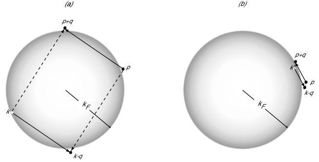
Figure 1: (a) A typical scattering process between electrons of the same spin orientation near the Fermi surface has contributions from both a “direct” (solid line) and an “exchange” (dotted line) term; (b) A special class of low momentum transfer processes gives the leading-order contribution to the scattering amplitude in 2D at high density.

Making use of the Fermi golden rule, we get pines ,

$$\frac{1}{\tau_{\sigma}^{(D)}}=2\pi \sum_{{\bf k},{\bf q}}\sum_{\sigma^{\prime}}W^{2}({\bf q}){\bar{n}}_{{\bf p}+{\bf q}\sigma}n_{\bf k\sigma^{\prime}}{\bar{n}}_{{\bf k}-{\bf q}\sigma^{\prime}}$$ (4)

$$\times\delta(\xi_{p}+\xi_{{\bf k}\sigma^{\prime}}-\xi_{{\bf k}-{\bf q}\sigma^{\prime}}-\xi_{{\bf p}+{\bf q}\sigma}),$$

and

$$\frac{1}{\tau_{\sigma}^{(EX)}}= -2\pi\sum_{{\bf k},{\bf q}}W({\bf p}-{\bf k}+{\bf q})W({\bf q}){\bar{n}}_{{\bf p}+{\bf q}\sigma}{\bar{n}}_{{\bf k}-{\bf q}\sigma}n_{{\bf k}\sigma}$$ (5)

$$\times\delta(\xi_{p}+\xi_{{\bf k}\sigma}-\xi_{{\bf k}-{\bf q}\sigma}-\xi_{{\bf p}+{\bf q}\sigma}),$$

where $W({\bf q})$ is the effective interaction between two quasiparticles, $n_{{\bf k}\sigma}=\frac{1}{e^{\beta\xi_{\bf k}}+1}$ the Fermi-Dirac distribution function at temperature $\beta=\frac{1}{k_{B}T}$, and we have set $\hbar=1$. The $\delta$-functions ensure the conservation of the energy in the collisions. Obviously, from Eqs. (4) and (5), one can see that the contribution from the “exchange” process tends to cancel that from the “direct” process.

As can be seen from Eq. (4), there are two types of collisions contributing to the “direct” term, the collisions with same-spin electrons ($\sigma^{\prime}=\sigma$), and those with opposite-spin electrons ($\sigma^{\prime}=-\sigma$). We denote the former $1/\tau_{\sigma\sigma}$, and the latter $1/\tau_{\sigma{\bar{\sigma}}}$, where ${\bar{\sigma}}=-\sigma$. It can be easily shown that

$$\frac{1}{\tau_{\sigma\sigma}^{(D)}}\geq-\frac{1}{\tau_{\sigma}^{(EX)}}.$$ (6)

In the paramagnetic state, one evidently has

$$\frac{1}{\tau_{\sigma\sigma}^{(D)}}=\frac{1}{\tau_{\sigma\bar{\sigma}}^{(D)}}.$$ (7)

Therefore,

$$\frac{1}{2\tau_{\sigma}^{(D)}}\geq-\frac{1}{\tau_{\sigma}^{(EX)}}.$$ (8)

The effective interaction $W({\bf q})$ between quasiparticles is short-ranged compared to the bare Coulomb potential due to the screening effects from the remaining electrons. Such screening effects are normally characterized by a screening wave vector $k_{s}$. Following this practice we approximate

$$W({\bf q})=\left\{\begin{array}[]{l}\frac{4\pi e^{2}}{q^{2}+k_{s}^{2}}~{}~{}~{}~{}~{}(3D){}\\ \frac{2\pi e^{2}}{q+k_{s}}~{}~{}~{}~{}~{}~{}(2D)~{},\end{array}\right.$$ (9)

where

$$k_{s}=\left\{\begin{array}[]{l}\sqrt{\frac{4k_{F}}{\pi a_{0}}}~{}~{}~{}~{}~{}(3D)\\ ~{}~{}~{}\frac{2}{a_{0}}~{}~{}~{}~{}~{}~{}~{}(2D)~{},\end{array}\right.$$ (10)

and $k_{F}$ and $a_{0}$ are the Fermi wave vector and the Bohr radius, respectively. At very low density, the screening wave vector becomes much larger than the Fermi wave vector. It can be shown that, in this limit,

$$\frac{1}{\tau_{\sigma\sigma}^{(D)}}=-\frac{1}{\tau_{\sigma}^{(EX)}},$$ (11)

or, in other words, by using Eq. (7),

$$\frac{1}{2\tau_{\sigma}^{(D)}}=-\frac{1}{\tau_{\sigma}^{(EX)}}.$$ (12)

Eq. (8) and the low density limit result of Eq. (12) are exact results, which, to the best of our knowledge, were not explicitly established before.

In what follows we will only consider the case of the paramagnetic electron liquid, which allows us to trivially dispose of the spin indices. Furthermore, by making the change of variable ${\bf k}\to{\bf k}+{\bf q}$ in the momentum summation in Eq. (5), and correspondingly, ${\bf k}\to-{\bf k}$ in Eq. (4), we rewrite Eqs. (4) and (5) as

$$\frac{1}{\tau^{(D)}}=2\pi \sum_{{\bf k},{\bf q}}\sum_{\sigma^{\prime}}W^{2}({\bf q}){\bar{n}}_{{\bf p}+{\bf q}}n_{\bf k}{\bar{n}}_{{\bf k}+{\bf q}}$$ (13)

$$\times\delta(\xi_{p}+\xi_{\bf k}-\xi_{{\bf k}+{\bf q}}-\xi_{{\bf p}+{\bf q}}),$$

and

$$\frac{1}{\tau^{(EX)}}= -2\pi\sum_{{\bf k},{\bf q}}W({\bf p}-{\bf k})W({\bf q}){\bar{n}}_{{\bf p}+{\bf q}}{\bar{n}}_{\bf k}n_{{\bf k}+{\bf q}}$$ (14)

$$\times\delta(\xi_{p}+\xi_{{\bf k}+{\bf q}}-\xi_{\bf k}-\xi_{{\bf p}+{\bf q}}).$$

By using the identity,

$$\frac{\Im m\chi_{0}(q,\omega)}{1-e^{-\beta\omega}}=-2\pi\sum_{\bf k}n_{\bf k}{\bar{n}}_{{\bf k}+{\bf q}}\delta(\omega+\xi_{\bf k}-\xi_{{\bf k}+{\bf q}}),$$ (15)

where $\chi_{0}(q,\omega)$ is the Lindhard function (i.e., the density-density response function of the non interacting electron gas), we rewrite $1/\tau^{(D)}$ in Eq. (13) as

$$\frac{1}{\tau^{(D)}} =-2\int_{-\infty}^{\infty}d\omega\frac{1}{[1+e^{\beta(\omega-\xi_{p})}][1-e^{-\beta\omega}]}$$ (16)

$$\times\sum_{\bf q}W^{2}({\bf q})\delta(\omega-\xi_{p}+\xi_{{\bf p}+{\bf q}})Im\chi_{0}(q,\omega).$$

In obtaining Eq. (16), we have also used the fact that

$${\bar{n}}_{{\bf p}+{\bf q}}\delta(\omega-\xi_{p}+\xi_{{\bf p}+{\bf q}})=\frac{1}{1+e^{\beta(\omega-\xi_{p})}}\delta(\omega-\xi_{p}+\xi_{{\bf p}+{\bf q}}).$$

Similarly, one has

$$\frac{1}{\tau^{(EX)}} =-2\pi\int_{-\infty}^{\infty}d\omega\frac{1}{1+e^{\beta(\omega-\xi_{p})}}\sum_{{\bf k},{\bf q}}W({\bf q}){\bar{n}}_{\bf k}n_{{\bf q}+{\bf k}}$$

$$\times\delta(\omega-\xi_{\bf k}+\xi_{{\bf q}+{\bf k}})\delta(\omega-\xi_{p}+\xi_{{\bf q}+{\bf p}})W({\bf p}-{\bf k}).$$

The fact that $1/\tau^{(D)}$ and $1/\tau^{(EX)}$ depend only of the magnitude of ${\bf p}$ allows us to average over the unit vector of ${\bf\hat{p}}=\frac{{\bf p}}{p}$ on the right hand side of Eqs. (16) and (II). To this end, we define

$$\Omega_{\pm}(q)\equiv\pm\frac{pq}{m}-\frac{q^{2}}{2m},$$ (19)

and use the fact that

$$\frac{1}{2^{d-1}\pi}\int d{\bf\hat{p}} \delta(\omega-\xi_{p}+\xi_{{\bf q}+{\bf p}})=\Theta(p,q)$$ (20)

$$\times\theta(\Omega_{+}(q)-\omega)\theta(\omega-\Omega_{-}(q))~{},$$

where $\theta(x)=1$ for $x>0$, and $\theta(x)=0$ for $x\leq 0$, and

$$\Theta(p,q)=\left\{\begin{array}[]{l}\frac{m}{2pq}~{},~{}~{}~{}~{}~{}~{}~{}~{}~{}~{}~{}~{}~{}~{}~{}~{}~{}~{}~{}~{}~{}(3D)\\ \frac{2m}{\pi\sqrt{4p^{2}q^{2}-(2m\omega+q^{2})^{2}}}~{},~{}~{}~{}(2D)~{}.\end{array}\right.$$ (21)

Therefore $1/\tau^{(D)}$ can be rewritten as

$$\frac{1}{\tau^{(D)}} = -2\int_{-\infty}^{\infty}d\omega\frac{1}{[1+e^{\beta(\omega-\xi_{p})}][1-e^{-\beta\omega}]}$$ (22)

$$\times \sum_{\bf q}W^{2}(q)\Im m\chi_{0}(q,\omega)\Theta(p,q)\theta(\Omega_{+}(q)-\omega)\theta(\omega-\Omega_{-}(q))~{}.$$

We note that this equation is not restricted to the regime of $k_{B}T\ll E_{F}$, but holds for arbitrary temperature.

In this paper, we are only interested in the case that $k_{B}T\ll E_{F}$, and therefore the Fermi energy $E_{F}$ is always well defined and $E_{F}\simeq\mu$. To perform the average over ${\bf\hat{p}}$ in Eq. (II), we use the fact that, for $k_{B}T,\xi_{p}\ll E_{F}$, the contribution to $1/\tau^{(EX)}$ only arises from the region in which $\xi_{\bf k},|\omega|\ll E_{F}$. Furthermore, the first $\delta$-function in Eq. (II) fixes the angle between ${\bf k}$ and ${\bf q}$ to be such as to satisfy the condition $\xi_{\bf k}-\xi_{{\bf q}+{\bf k}}=\omega\approx 0$. With this in mind, one obtains

$$\frac{1}{2^{d-1}\pi} \int d{\bf\hat{p}}\delta(\omega-\xi_{p}+\xi_{{\bf q}+{\bf p}})W({\bf p}-{\bf k})$$ (23)

$$=\Phi(p,q)\theta(\Omega_{+}(q)-\omega)\theta(\omega-\Omega_{-}(q)),$$

where

$$\Phi(p,q)=\left\{\begin{array}[]{l}\frac{m}{2pqk_{s}}\frac{4\pi e^{2}}{\sqrt{k_{s}^{2}+4k_{F}^{2}-q^{2}}}~{},~{}~{}~{}~{}~{}~{}~{}~{}~{}~{}~{}~{}~{}~{}~{}~{}~{}~{}~{}~{}~{}~{}~{}~{}~{}~{}~{}~{}(3D)\\ \frac{me^{2}}{\sqrt{p^{2}q^{2}-(m\omega+q^{2}/2)^{2}}}\left[\frac{1}{k_{s}}+\frac{1}{\sqrt{4k_{F}^{2}-q^{2}}+k_{s}}\right]~{},~{}~{}(2D)~{}.\end{array}\right.$$ (24)

A detailed derivation of this key result is presented in the Appendix. Thus finally

$$\frac{1}{\tau^{(EX)}} = \int_{-\infty}^{\infty}d\omega\frac{1}{[1+e^{\beta(\omega-\xi_{p})}][1-e^{-\beta\omega}]}$$ (25)

$$\times \sum_{\bf q}W(q)\Im m\chi_{0}(q,\omega)\Phi(p,q)\theta(\Omega_{+}(q)-\omega)\theta(\omega-\Omega_{-}(q)).$$

III The inverse lifetime in 3D

The theory of the electron inelastic lifetime in 3D is rather well established quinn ; ritchie at zero temperature. However, no analytical expression including the exchange has been presented so far, even though Kleinman kleinman , and later Penn penn , have reported numerical calculations of the exchange contribution. This deficiency is remedied in the present section. Our calculation is done at nonzero temperature, with zero temperature as a special case.

In 3D, Eq. (22) becomes

$$\frac{1}{\tau^{(D)}} = -\frac{m}{2(2\pi)^{3}p}\int_{-\infty}^{\infty}d\omega\frac{2}{[1+e^{\beta(\omega-\xi_{p})}][1-e^{-\beta\omega}]}$$ (26)

$$\times \int d{\bf q}W^{2}(q)\frac{1}{q}\Im m\chi_{0}(q,\omega)\theta(\Omega_{+}(q)-\omega)\theta(\omega-\Omega_{-}(q)).$$

We are interested in the case that $k_{B}T,\xi_{p}\ll E_{F}$. Therefore we only need consider the region of $\omega\ll E_{F}$, in which,

$$Im\chi_{0}(q,\omega)=-\frac{m^{2}\omega}{2\pi q}\theta(2k_{F}-q).$$ (27)

Substituting Eq. (27) into (26) leads to

$$\frac{1}{\tau^{(D)}}=\frac{m^{3}}{(2\pi)^{3}p} \int_{-\infty}^{\infty}d\omega\frac{2\omega}{[1+e^{\beta(\omega-\xi_{p})}][1-e^{-\beta\omega}]}$$ (28)

$$\times\int_{0}^{2k_{F}}dqW^{2}(q).$$

The integrations over $q$ and $\omega$ can be carried through, and one obtains

$$\frac{1}{\tau^{(D)}}=\frac{m^{3}e^{4}}{\pi pk_{s}^{3}}\frac{\pi^{2}k_{B}^{2}T^{2}+\xi_{p}^{2}}{1+e^{-\beta\xi_{p}}}\biggl{[}\frac{\lambda}{\lambda^{2}+1}+\tan^{-1}\lambda\biggr{]},$$ (29)

where $\lambda=\frac{2k_{F}}{k_{s}}$.

Next we move to evaluate the contribution from the exchange process. In 3D, Eq. (25) becomes

$$\frac{1}{\tau^{(EX)}} = \frac{\pi e^{2}m}{(2\pi)^{3}pk_{s}}\int_{-\infty}^{\infty}d\omega\frac{2}{1+e^{\beta(\omega-\xi_{p})}][1-e^{-\beta\omega}]}$$ (30)

$$\times \int d{\bf q}W(q)\frac{\Im m\chi_{0}(q,\omega)}{q\sqrt{k_{s}^{2}+4k_{F}^{2}-q^{2}}}\theta(\Omega_{+}(q)-\omega)\theta(\omega-\Omega_{-}(q)).$$

By using Eq. (27), one has

$$\frac{1}{\tau^{(EX)}}=- \frac{m^{3}e^{2}}{(2\pi)^{2}pk_{s}}\int_{-\infty}^{\infty}d\omega\frac{2\omega}{[1+e^{\beta(\omega-\xi_{p})}][1-e^{-\beta\omega}]}$$ (31)

$$\times\int_{0}^{2k_{F}}dqW(q)\frac{1}{\sqrt{k_{s}^{2}+4k_{F}^{2}-q^{2}}}.$$

After carrying out the integrations, one obtains the final result,

$$\frac{1}{\tau^{(EX)}} =-\frac{m^{3}e^{4}}{\pi pk_{s}^{3}}\frac{\pi^{2}k_{B}^{2}T^{2}+\xi_{p}^{2}}{1+e^{-\beta\xi_{p}}}$$ (32)

$$\times\frac{1}{\sqrt{\lambda^{2}+2}}\biggl{[}\frac{\pi}{2}-\tan^{-1}\biggl{(}\frac{1}{\lambda}\sqrt{\frac{1}{\lambda^{2}+2}}\biggr{)}\biggr{]}.$$

We plot the ratio of $1/\tau^{(EX)}$ to $1/\tau^{(D)}$ vs the Wigner-Seitz radius $r_{s}$ in Fig. 2. Notice that at very high density, $|1/\tau^{(EX)}|\ll|1/\tau^{(D)}|$, and the direct-process-only theory is then relatively good. On the other hand, at low density, $1/\tau^{(EX)}=-1/2\tau^{(D)}$, which agrees with the general conclusion of Eq. (12). The contribution from exchange processes therefore cannot be ignored in most density range.

Figure 2: The ratio of $1/\tau^{(EX)}$ over $1/\tau^{(D)}$ via $r_{s}$ in 3D.

In the limiting case of small excitation energy, $\xi_{p}\ll k_{B}T\ll E_{F}$, Eq. (29) reduces to

$$\frac{1}{\tau^{(D)}}=\frac{\pi m^{3}e^{4}}{2pk_{s}^{3}}k_{B}^{2}T^{2}\biggl{[}\frac{\lambda}{\lambda^{2}+1}+\tan^{-1}\lambda\biggr{]}.$$ (33)

In the opposite of very low temperature, $k_{B}T\ll\xi_{p}\ll E_{F}$, one has

$$\frac{1}{\tau^{(D)}}=\frac{m^{3}e^{4}}{\pi pk_{s}^{3}}\xi_{p}^{2}\biggl{[}\frac{\lambda}{\lambda^{2}+1}+\tan^{-1}\lambda\biggr{]}.$$ (34)

In the high density limit, $\lambda\to\infty$, Eq. (34) becomes

$$\frac{1}{\tau^{(D)}}=\frac{m^{3}e^{4}}{2pk_{s}^{3}}\xi_{p}^{2},$$ (35)

a result obtained earlier by Quinn and Ferrell quinn .

IV The inverse lifetime in 2D

As mentioned in the introduction, there is still some disagreement among the results of previous calculations of $1/\tau_{e}$ in 2D. The main purpose of this section is to exactly evaluate the prefactors of $1/\tau^{(D)}$ and $1/\tau^{(EX)}$ in 2D, and at the same time attempt to clarify the origin of those disagreements. We present our derivations in the two different regimes of $k_{B}T\ll\xi_{p}\ll E_{F}$ and $\xi_{p}\ll k_{B}T\ll E_{F}$ separately. For greater clarity, we also show our derivations for the “direct” and “exchange” contributions in separate subsections.

IV.1 $k_{B}T\ll\xi_{p}$: Direct process

In 2D, for $k_{B}T\ll\xi_{p}\ll E_{F}$, Eq. (22) becomes

$$\frac{1}{\tau^{(D)}}= -\frac{2m}{\pi^{2}}\int_{0}^{\xi_{p}}d\omega\biggl{[}\int_{-k_{F}+\sqrt{k_{F}^{2}+2m\omega}}^{k_{F}-\sqrt{k_{F}^{2}-2m\omega}}dq$$ (36)

$$+\int_{k_{F}-\sqrt{k_{F}^{2}-2m\omega}}^{k_{F}+\sqrt{k_{F}^{2}-2m\omega}}dq+\int_{k_{F}+\sqrt{k_{F}^{2}-2m\omega}}^{k_{F}+\sqrt{k_{F}^{2}+2m\omega}}dq\biggr{]}$$

$$\times qW^{2}(q)\frac{\Im m\chi_{0}(q,\omega)}{\sqrt{4p^{2}q^{2}-(2m\omega+q^{2})^{2}}}.$$

The three regions of integration, at a given value of $\omega$ are shown in Fig. 3.

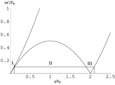
Figure 3: The three regions of integration over $q$, at given $\omega$, in Eq. (36) are labelled as I, II and III respectively. Only region II contributes to the leading order in 2D.

It can be shown (Damico ) that the first and the third terms in the square bracket make contributions of the order of $O(\xi_{p}^{2})$, but not to the leading order of $O(\xi_{p}^{2}\ln\xi_{p})$, which arises only from the second term. Hereafter we therefore focus only on the calculation of the second term.

The small $\omega$ expression for $\Im m\chi_{0}(q,\omega)$ in 2D is

$$\Im m\chi_{0}(q,\omega)=-\frac{2m^{2}\omega}{\pi q\sqrt{4k_{F}^{2}-q^{2}}}.$$ (37)

Therefore we obtain

$$\frac{1}{\tau^{(D)}}=\frac{4m^{3}}{\pi^{3}}\int_{0}^{\xi_{p}}\omega d\omega Q_{1}(\omega),$$ (38)

where

$$Q_{1}(\omega)=\int_{k_{F}-\sqrt{k_{F}^{2}-2m\omega}}^{k_{F}+\sqrt{k_{F}^{2}-2m\omega}}dqW^{2}(q)\frac{1}{q(4k_{F}^{2}-q^{2})},$$ (39)

or, to the leading order,

$$Q_{1}(\omega)=\int_{m\omega/k_{F}}^{2k_{F}-m\omega/k_{F}}dqW^{2}(q)\frac{1}{q(4k_{F}^{2}-q^{2})}.$$ (40)

Evidently, the integration in Eq. (40) has a logarithmic divergence at both the upper and lower limits. To the leading order, $Q_{1}(\omega)$ can be evaluated as

$$Q_{1}(\omega)=-\frac{1}{8k_{F}^{2}}[2W^{2}(0)+W^{2}(2k_{F})]\ln\frac{m\omega}{k_{F}^{2}}~{}.$$ (41)

Substituting Eq. (41) into (38), and performing the integration over $\omega$, we finally arrive at

$$\frac{1}{\tau^{(D)}}=\frac{\xi_{p}^{2}}{4\pi E_{F}}\left[\bar{W}^{2}(0)+\frac{1}{2}\bar{W}^{2}(2k_{F})\right]\ln\frac{2E_{F}}{\xi_{p}}~{},$$ (42)

where we have defined the dimensionless quantity

$$\bar{W}(q)\equiv\frac{m}{\pi}W(q)~{}.$$ (43)

The quantity in the square brackets of Eq. (42) can be expressed in terms of the Wigner-Seitz radius $r_{s}$ as follows:

$$\bar{W}^{2}(0)+\frac{1}{2}\bar{W}^{2}(2k_{F})=1+\frac{1}{2}\left(\frac{r_{s}}{r_{s}+\sqrt{2}}\right)^{2}~{}.$$ (44)

The fact that Eq. (40) also has a logarithmic contribution from the upper limit of integration at $q\simeq 2k_{F}$ was missed in almost all previous analytical calculations. This is one of the main reasons leading to errors in the numerical prefactor of the lifetime. The second term in the square brackets of Eq. (42) is absent in the works of Refs. (giuliani ; zheng ; reizer ), while it is over-appreciated in the work of Jungwirth and MacDonald jungwirth , where the factor $\frac{1}{2}$ in front of $\bar{W}^{2}(2k_{F})$ is replaced by $1$. All these formulas are, of course, equivalent in the high-density limit ($r_{s}\to 0$).

Except for the work by Reizer and Wilkins reizer , all the calculations cited above in 2D explicitly consider only the direct process, without taking account of the exchange process, which we deal with in the next subsection.

IV.2 $k_{B}T\ll\xi_{p}$: Exchange process

In 2D, for $k_{B}T\ll\xi_{p}\ll E_{F}$, Eq. (25) becomes

$$\frac{1}{\tau^{(EX)}}= \frac{2m}{(2\pi)^{2}}\int_{0}^{\xi_{p}}d\omega\biggl{[}\int_{-k_{F}+\sqrt{k_{F}^{2}+2m\omega}}^{k_{F}-\sqrt{k_{F}^{2}-2m\omega}}dq$$ (45)

$$+\int_{k_{F}-\sqrt{k_{F}^{2}-2m\omega}}^{k_{F}+\sqrt{k_{F}^{2}-2m\omega}}dq+\int_{k_{F}+\sqrt{k_{F}^{2}-2m\omega}}^{k_{F}+\sqrt{k_{F}^{2}+2m\omega}}dq\biggr{]}$$

$$\times qW(q)[W(0)+W(\sqrt{4k_{F}^{2}-q^{2}})]$$

$$\times\frac{\Im m\chi_{0}(q,\omega)}{\sqrt{4p^{2}q^{2}-(q^{2}+2m\omega)^{2}}}.$$

Again only the second term in the square bracket contributes to the leading order. Thus,

$$\frac{1}{\tau^{(EX)}}=-\frac{4m^{3}}{\pi(2\pi)^{2}}\int_{0}^{\xi_{p}}d\omega\omega Q_{2}(\omega),$$ (46)

where

$$Q_{2}(\omega)= \int_{k_{F}-\sqrt{k_{F}^{2}-2m\omega}}^{k_{F}+\sqrt{k_{F}^{2}-2m\omega}}dq\frac{1}{q(4k_{F}^{2}-q^{2})}$$ (47)

$$\times W(q)[W(0)+W(\sqrt{4k_{F}^{2}-q^{2}})].$$

To the leading order,

$$Q_{2}(\omega)=-\frac{1}{4k_{F}^{2}}W(0)[W(0)+2W(2k_{F})]\ln\frac{m\omega}{k_{F}^{2}}.$$ (48)

Substituting Eq. (48) into Eq. (46) and performing the integration over $\omega$, we arrive at

$$\frac{\hbar}{\tau^{(EX)}}=\frac{\xi_{p}^{2}}{16\pi E_{F}}\bar{W}(0)[\bar{W}(0)+2\bar{W}(2k_{F})]\ln\frac{\xi_{p}}{2E_{F}}.$$ (49)

In Fig. 4, we show the ratio of $1/\tau^{(EX)}$ to $1/\tau^{(D)}$ vs $r_{s}$. The remarkable fact is that, at variance with the 3D case, this ratio does not vanish for $r_{s}\to 0$. The reason for this difference can be understood as follows. In 3D a typical scattering process near the Fermi surface, such as the one shown in Fig. 1(a), involves two particles that are well separated (by a wave vector of the order of $2k_{F}$) in momentum space. The direct scattering amplitude for such a process is maximum when the momentum transfer $q$ is much smaller than $k_{F}$, and is thus typically proportional to $W(0)$. The exchange scattering amplitude, on the other hand, is of the order of $W(2k_{F})$ for all values of $q$: hence the ratio of $1/\tau^{(EX)}$ to $1/\tau^{(D)}$ goes as $\frac{W(0)W(2k_{F})}{W(0)^{2}}$, which vanishes for $r_{s}\to 0$. The reason why this argument fails in 2D is that the logarithmic contribution to the inverse lifetime in the high density limit does not arise from typical scattering processes, but rather, from special ones in which the two colliding particles are very close in momentum space (see Fig. 1(b)): hence the direct and the scattering amplitude are comparable, and give similar contributions to the inverse lifetime. A careful analysis of the integrals involved shows that in the high density limit, the exchange contribution cancels $\frac{1}{4}$ of the direct contribution to the inverse lifetime. This result is at variance with that of Ref. reizer , according to which the exchange contribution cancels $\frac{1}{2}$ of the direct one. We find that the relation $1/\tau^{(EX)}=-1/2\tau^{(D)}$ holds only in the low density limit (see Eq. (12) and Fig. 4), where the weak coupling theory is not reliable.

Combining direct and exchange contributions in a single formula we finally find that

$$\frac{1}{\tau_{e}}=\frac{\xi_{p}^{2}}{4\pi E_{F}}\left[\frac{3}{4}\bar{W}(0)^{2}+\frac{1}{2}\bar{W}(2k_{F})^{2}-\frac{1}{2}\bar{W}(0)\bar{W}(2k_{F})\right]\ln\frac{2E_{F}}{\xi_{p}}~{},$$ (50)

where the quantity in the square brackets is given by

$$\frac{3}{4}-\frac{r_{s}}{\sqrt{2}(r_{s}+\sqrt{2})^{2}}~{}.$$ (51)

Thus in the high density limit the total inverse lifetime differs by a factor $\frac{3}{4}$ from the result of the direct-scattering-only calculation, and by a factor $\frac{3}{2}$ from the result of Ref. (reizer ).

Figure 4: The ratio of $1/\tau^{(EX)}$ over $1/\tau^{(D)}$ via $r_{s}$ in 2D.

IV.3 $\xi_{p}\ll k_{B}T$: Direct process

For $\xi_{p}\ll k_{B}T\ll E_{F}$, Eq. (22) becomes

$$\frac{1}{\tau^{(D)}}=-\frac{m}{\pi^{2}} \biggl{[}\int_{-\infty}^{0}d\omega\int_{-q_{-}(\omega)}^{q_{+}(\omega)}dq$$ (52)

$$+\int_{0}^{\mu+\xi_{p}}d\omega\int_{q_{-}(\omega)}^{q_{+}(\omega)}dq\biggl{]}$$

$$\times\frac{1}{sh\beta\omega}\frac{qW^{2}(q)\Im m\chi_{0}(q,\omega)}{\sqrt{4p^{2}q^{2}-(2m\omega+q^{2})^{2}}},$$

where $q_{\pm}(\omega)$ are the solutions of the equation $\Omega_{+}(q)=\omega$,

$$q_{\pm}(\omega)=[p\pm\sqrt{p^{2}-2m\omega}].$$ (53)

Again, only the regime of $\omega\ll E_{F}$ contributes to $1/\tau_{p}^{(D)}$ to the accuracy of the leading order. Thus, by using Eq. (37), one has

$$\frac{1}{\tau^{(D)}}= \frac{2m^{3}}{\pi^{3}}\int_{-\infty}^{\infty}d\omega\frac{\omega}{sh\beta\omega}\biggl{[}\int_{-k_{F}+\sqrt{k_{F}^{2}+2m|\omega|}}^{k_{F}-\sqrt{k_{F}^{2}-2m|\omega|}}dq$$ (54)

$$+\int_{k_{F}-\sqrt{k_{F}^{2}-2m|\omega|}}^{k_{F}+\sqrt{k_{F}^{2}-2m|\omega|}}dq+\int_{k_{F}+\sqrt{k_{F}^{2}-2m|\omega|}}^{k_{F}+\sqrt{k_{F}^{2}+2m|\omega|}}dq\biggr{]}$$

$$\times W^{2}(q)\frac{1}{\sqrt{4p^{2}q^{2}-(2m\omega+q^{2})^{2}}}$$

$$\times\frac{1}{\sqrt{4k_{F}^{2}-q^{2}}}.$$

Once again only the second term in the bracket makes contribution to the leading order, and we find

$$\frac{1}{\tau^{(D)}}= \frac{2m^{3}}{\pi^{3}}\int_{-\infty}^{\infty}d\omega\frac{\omega}{sh\beta\omega}Q_{1}(\omega),$$ (55)

where $Q_{1}(\omega)$ is defined in Eq. (40) and evaluated in Eq. (41). Therefore

$$\frac{1}{\tau^{(D)}}= -\frac{m^{3}}{4\pi^{3}k_{F}^{2}}[2W^{2}(0)+W^{2}(2k_{F})]$$ (56)

$$\times\int_{-\infty}^{\infty}d\omega\frac{\omega}{sh\beta\omega}\ln\frac{m\omega}{k_{F}^{2}},$$

which can be further evaluated leading to

$$\frac{\hbar}{\tau^{(D)}}=\frac{\left(\pi k_{B}T\right)^{2}}{8\pi E_{F}}\left[\bar{W}^{2}(0)+\frac{1}{2}\bar{W}^{2}(2k_{F})\right]\ln\frac{2E_{F}}{k_{B}T}.$$ (57)

As in the low-temperature case, the second term in the square brackets of this equation was missed in almost all the previous theories except the one by Jungwirth and MacDonald jungwirth , which, however, overestimates it by a factor $2$. Without the second term in the square bracket Eq. (57) would agree with the expression obtained by Zheng and Das Sarma zheng and by Reizer and Wilkins reizer , but it would be four times smaller than the result of Fukuyama and Abrahams fukuyama , and $\frac{\pi^{2}}{4}$ times larger than the result of Giuliani and Quinn giuliani .

IV.4 $\xi_{p}\ll k_{B}T$: Exchange process

In 2D, for $k_{B}T\gg\xi_{p}$, Eq. (25) becomes

$$\frac{1}{\tau^{(EX)}}= \frac{m}{4\pi^{2}}\biggl{[}\int_{-\infty}^{0}d\omega\int_{-q_{-}(\omega)}^{q_{+}(\omega)}dq$$ (58)

$$+\int_{0}^{\mu+\xi_{p}}d\omega\int_{q_{-}(\omega)}^{q_{+}(\omega)}dq\biggl{]}$$

$$\times\frac{1}{sh\beta\omega}\frac{\Im m\chi_{0}(q,\omega)}{\sqrt{4p^{2}q^{2}-(2m\omega+q^{2})^{2}}}$$

$$\times W(q)q[W(0)+W(\sqrt{4k_{F}^{2}-q^{2}})].$$

Proceeding as in the previous section we rewrite this as

$$\frac{1}{\tau^{(EX)}}=-\frac{m^{3}}{2\pi^{3}}\int_{-\infty}^{\infty}d\omega\frac{\omega}{sh\beta\omega}Q_{2}(\omega),$$ (59)

where $Q_{2}(\omega)$ is defined in Eq. (47) and evaluated in Eq. (48). Therefore

$$\frac{1}{\tau^{(EX)}}= \frac{m^{3}}{8\pi^{3}k_{F}^{2}}W(0)[W(0)+2W(2k_{F})]$$ (60)

$$\times\int_{-\infty}^{\infty}d\omega\frac{\omega}{sh\beta\omega}\ln\frac{m\omega}{k_{F}^{2}}~{},$$

which can be, to the leading order, further simplified to

$$\frac{1}{\tau^{(EX)}}=\frac{\left(\pi k_{B}T\right)^{2}}{32\pi E_{F}}\bar{W}(0)[\bar{W}(0)+2\bar{W}(2k_{F})]\ln\frac{k_{B}T}{2E_{F}}~{}.$$ (61)

The ratio of $1/\tau^{(EX)}$ to $1/\tau^{(D)}$ is therefore found to be the same as that in the case of $k_{B}T\ll\xi_{p}$, which has been plotted in Fig. 4.

Combination of $1/\tau^{(D)}$ in Eq. (57) and $1/\tau^{(EX)}$ in Eq. (61) thus yields

$$\frac{1}{\tau_{e}}=-\frac{\left(\pi k_{B}T\right)^{2}}{32\pi E_{F}}[3\bar{W}^{2}(0)+2\bar{W}^{2}(2k_{F})-2\bar{W}(0)\bar{W}(2k_{F})]\ln\frac{k_{B}T}{2E_{F}}~{}.$$ (62)

Notice the difference between the above result and the one obtained in Ref. reizer .

V Comparison with Experimental results in 2D

Consider two identical 2D electron liquids in closely spaced quantum wells between which a small potential difference $V$ is maintained. We expect a small tunneling current between the layers. However, as Fig. 5 shows, no tunneling is possible in the absence of impurities and electron interactions. This is because under those unrealistic assumptions both the energy and the momentum of the electron must be conserved during tunneling, and there are simply no states satisfying these conditions.

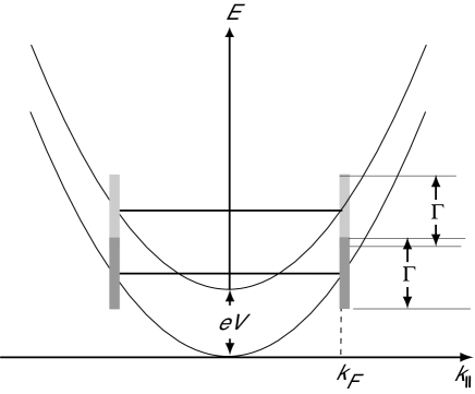
Figure 5: Momentum- and energy-conserving tunneling between two identical free-electron bands separated by a potential difference $eV$ is possible only if the spectral width of the single particle states in each band (indicated by the shaded regions) is at least as large as $eV$.

The situation changes profoundly if electron-electron interactions are allowed. Now momentum is still conserved (if impurity scattering and surface roughness are negligible) but the energy of the electron quasiparticle is no longer a well defined quantity, due to the possibility of inelastic scattering processes involving other electrons in each quantum well. As a result, tunneling becomes possible in a region of voltages $-\Gamma<V<\Gamma$ where $\Gamma$ is the width at half-maximum of the plane-wave spectral function in a well murphy , i.e.,

$$A(E,\xi_{p})=\frac{1}{2\pi}\frac{\Gamma(\xi_{p},T)}{(E-\xi_{p})^{2}+[\Gamma(\xi_{p},T)/2]^{2}}~{}.$$ (63)

From the well-known relation $A(E,\xi_{p})=-\frac{1}{\pi}\Im mG_{ret}(E,\xi_{p})$, where $G_{ret}(E,\xi_{p})$ is the retarded Green’s function, one can show that the spectral width $\Gamma$ is just the inverse of the lifetime of a plane wave state, which is the sum of the lifetimes of electron and hole quasiparticles in the following manner:(jungwirth ; mahan

$$\Gamma(\xi_{p},T)=\frac{1}{\tau_{e}(\xi_{p},T)}+\frac{1}{\tau_{h}(\xi_{p},T)}.$$ (64)

The principle of detailed balance demands

$$\frac{n(\xi_{p},T)}{\tau_{e}}=\frac{1-n(\xi_{p},T)}{\tau_{h}}~{},$$ (65)

where $n(\xi_{p},T)$ is the thermal occupation number at temperature $T$. If we assume $\xi_{p}\ll k_{B}T$ and approximate $\Gamma(\xi_{p},T)$ by $\Gamma(\xi_{p}=0,T)$, we see from the above equations that the half-width at half-maximum of the tunneling conductance peak is expressed in terms of the electron quasiparticle lifetime as follows:

$$\Gamma=\frac{2}{\tau_{e}(0,T)}~{}.$$ (66)

We can now attempt a comparison between the experimental values of $\Gamma$ from Ref. (murphy ) and the theoretical values of $\frac{2}{\tau_{e}(0,T)}$. This is shown in Fig. 6. It must be kept in mind that, in order to perform a meaningful comparison, one must first subtract from the experimental data a (presumably) temperature-independent constant due to residual disorder. The value of this constant is determined by the condition that $\Gamma$ tend to zero for $T\to 0$. Even after this subtraction we see that the theoretical curve lies well below the experimental data. Furthermore, the shortcomings in Refs. jungwirth ; zheng as revealed in this paper imply that the “excellent agreement” with experiment claimed in those papers is overly optimistic, as pointed out earlier by Reizer and Wilkins reizer .

Figure 6: Electron relaxation rate $\Gamma$ in 2D. Experimental data are from Ref. murphy , calculated ones are from Eq. (62). Here $T_{F}=E_{F}/k_{B}$.

We note that all derivations presented in this paper are to the accuracy of the leading logarithmic term. Calculations including higher order terms might bring in a better agreement with the experimental data. However, it seems too optimistic to believe that the huge difference (roughly a factor $4$) between theory and experiment is totally due to such higher order contributions. The size of the discrepancy suggests that there might be other factors playing a role, like the finite width of the quasi-two-dimensional system, electron-impurity scattering, electron-phonon scattering, and surface roughness. While the inclusion of these effects may help to produce better agreement with experiments, it remains a great challenge for experimentalists to device the conditions that will eventually allow them to probe the truly intrinsic behavior of the electron liquid.

VI Acknowledgements

We gratefully acknowledge support by NSF grants DMR-0074959 and DMR-0313681. We especially thank Gabriele Giuliani for many valuable discussions.

VII Appendix

In this appendix, we give the details of the derivation of Eq. (23). To this end, we denote the left hand side of Eq. (23) as $A_{3}$ and $A_{2}$ for 3D and 2D cases, respectively. In 3D, $A_{3}$ can be rewritten as

$$A_{3}=e^{2}\int_{0}^{\pi}d\theta^{\prime}\sin\theta^{\prime}\int_{0}^{2\pi}d\phi^{\prime}\delta\left(\omega+\frac{pq\cos\theta^{\prime}}{m}+\frac{q^{2}}{2m}\right)$$

$$\frac{1}{p^{2}+k^{2}+k_{s}^{2}-2pk[\cos\theta\cos\theta^{\prime}+\sin\theta\sin\theta^{\prime}\cos(\phi-\phi^{\prime})]}$$

where $(\theta,\phi)$ and $(\theta^{\prime},\phi^{\prime})$ are the spherical angles of ${\bf k}$ and ${\bf p}$, respectively, relative to ${\bf q}$. Carrying through the $\phi^{\prime}$ integration, one obtains

$$A_{3}=2\pi e^{2}\int_{-1}^{1}dx\delta\left(\omega+\frac{pqx}{m}+\frac{q^{2}}{2m}\right)$$

$$\frac{1}{\sqrt{(p^{2}+k^{2}+k_{s}^{2}+2pk\cos\theta x)^{2}-4(pk\sin\theta)^{2}(1-x^{2})}}$$

The integral in the above equation is trivial due to the $\delta$ function, and it leads to

$$A_{3}=\frac{2\pi me^{2}\theta(\Omega_{+}(q)-\omega)\theta(\omega-\Omega_{-}(q))}{pq\sqrt{[p^{2}+k^{2}+k_{s}^{2}-{\bf k}\cdot{\bf q}]^{2}-[k^{2}-({\bf k}\cdot{\bf\hat{q}})^{2}][4p^{2}-q^{2}]}}$$

where we have used the fact that $2m\omega\ll k_{s}^{2}$ Putting in this expression the approximate equalities $k\sim p\sim k_{F}$ and ${\bf k}\cdot{\bf q}\sim-\frac{q^{2}}{2}$ (which follows from the condition $\xi_{\bf k}-\xi_{{\bf q}+{\bf k}}=\omega\simeq 0$ due to the first $\delta$-function in Eq. (II)) one easily arrives at Eq. (23) in the 3D case.

In 2D, $A_{2}$ can be explicitly written as

$$A_{2}=e^{2}\int_{0}^{2\pi}d\phi^{\prime}\delta(\omega+pq\cos\phi^{\prime}/m+q^{2}/2m)$$

$$\frac{1}{\sqrt{p^{2}+k^{2}-2pk\cos(\phi-\phi^{\prime})}+k_{s}}$$ (70)

or,

$$A_{2}=e^{2}\int_{0}^{\pi}d\phi^{\prime}\delta(\omega+pq/m\cos\phi^{\prime}+q^{2}/2m)$$

$$\biggl{[}\frac{1}{\sqrt{p^{2}+k^{2}-2pk\cos(\phi-\phi^{\prime})}+k_{s}}$$

$$+\frac{1}{\sqrt{p^{2}+k^{2}-2pk\cos(\phi+\phi^{\prime})}+k_{s}}\biggr{]}$$ (71)

Carrying out the integration over $\phi^{\prime}$ yields,

$$A_{2}=\frac{me^{2}\theta(\Omega_{+}(q)-\omega)\theta(\omega-\Omega_{-}(q))}{\sqrt{p^{2}q^{2}-(m\omega+q^{2}/2)^{2}}}$$

$$\left(\frac{1}{\sqrt{p^{2}+k^{2}+{\bf k}\cdot{\bf q}-\sqrt{[k^{2}-({\bf k}\cdot{\bf\hat{q}})^{2}][4p^{2}-q^{2}]}}+k_{s}}\right.$$

$$\left.+\frac{1}{\sqrt{p^{2}+k^{2}+{\bf k}\cdot{\bf q}+\sqrt{[k^{2}-({\bf k}\cdot{\bf\hat{q}})^{2}][4p^{2}-q^{2}]}}+k_{s}}\right)$$

Substituting, as in the 3D case, the approximate equalities, $k\sim p\sim k_{F}$ and ${\bf k}\cdot{\bf q}\sim-\frac{q^{2}}{2}$ one finally arrives at Eq. (23) in 2D.

References

- (1) D. Pines and P. Nozières, The Theory of Quantum Liquids (Benjamin, New York, 1996), Vol. 1.
- (2) G. F. Giuliani and J. J. Quinn, Phys. Rev. B 26, 4421 (1982).
- (3) K. K. Choi, D. C. Tsui, and K. Alavi, Phys. Rev. B 36, 7751 (1987).
- (4) A. Yacoby, U. Sivan, C. P. Umbach, and J. M. Hong, Phys. Rev. Lett. 66, 1938 (1991).
- (5) Y. Kawaji, S. Yamada, and H. Nakano, Appl. Phys. Lett. 56, 2123 (1990).
- (6) Y. Berk, A. Kamenev, A. Palevski, L. N. Pfeiffer, and K. W. West, Phys. Rev. B 51, 2604 (1995).
- (7) S. Q. Murphy, J. P. Eisenstein, L. N. Pfeiffer, and K. W. West, Phys. Rev. B 52, 14825 (1995).
- (8) M. Slutzky, O. Entin-Wohlman, Y. Berk, A. Palevski, and H. Shtrikman, Phys. Rev. B 53, 4065 (1996).
- (9) J. J. Quinn and R. A. Ferrell, Phys. Rev. 112, 812 (1958).
- (10) R. H. Ritchie and J. C. Ashley, J. Phys. Chem. Solids, 26, 1689 (1965).
- (11) L. Kleinman, Phys. Rev. B 3, 2982 (1971).
- (12) D. R. Penn, Phys. Rev. B 22, 2677 (1980).
- (13) H. Fukuyama and E. Abrahams, Phys. Rev. B 27, 5976 (1983).
- (14) A. V. Chaplik, Zh. Exsp. Teor. Fiz. 60, 1845 (1971) [Sov. Phys. JETP, 33, 997 (1971)]
- (15) C. Hodges, H. Smith, and J. W. Wilkins, Phys. Rev. B 4, 302 (1971).
- (16) G. Fasol, Appl. Phys. Lett. 59, 2430 (1991).
- (17) T. Jungwirth and A. H. MacDonald, Phys. Rev. B 53, 7403 (1996).
- (18) L. Zheng and S. Das Sarma, Phys. Rev. B 53, 9964 (1996).
- (19) D. Menashe and B. Laikhtman, Phys. Rev. B 54, 11561 (1996).
- (20) M. Reizer and J. W. Wilkins, Phys. Rev. B 55 R7363 (1997).
- (21) G. D. Mahan, Many-Particle Physics (Plenum, New York, 1981).
- (22) I. D’Amico and G. Vignale, Phys. Rev. B 68, 045307 (2003).