Charge transport in a quantum electromechanical system

Abstract

We describe a quantum electromechanical system(QEMS) comprising a single quantum dot harmonically bound between two electrodes and facilitating a tunneling current between them. An example of such a system is a fullerene molecule between two metal electrodes [Park et al. Nature, 407, 57 (2000)]. The description is based on a quantum master equation for the density operator of the electronic and vibrational degrees of freedom and thus incorporates the dynamics of both diagonal (population) and off diagonal (coherence) terms. We derive coupled equations of motion for the electron occupation number of the dot and the vibrational degrees of freedom, including damping of the vibration and thermo-mechanical noise. This dynamical description is related to observable features of the system including the stationary current as a function of bias voltage.

I Introduction

A quantum electromechanical system (QEMS) is a submicron electromechanical device fabricated through state-of-the-art nanofabricationroukes . Typically, such devices comprise a mechanical oscillator (a singly or doubly clamped cantilever) with surface wires patterned through shadow mask metal evaporation. The wires can be used to drive the mechanical system by carrying an AC current in an external static magnetic field. Surface wires can also be used as motion transducers through induced EMFs as the substrate oscillates in the external magnetic field. Alternatively the mechanical resonators can form an active part of a single electron transducer, such as one plate of a capacitively coupled single electron transistorknobel-clleland ; Schwab04 . These devices have been proposed as sensitive weak force probes with the potential to achieve single spin detectionspin-detection ; Brun03 . However they are of considerable interest in their own right as nano-fabricated mechanical resonators capable of exhibiting quantum noise features, such as squeezing and entanglement quantum-effects .

In order to observe quantum noise in a QEMS device we must recognize that these devices are open quantum systems and explicitly describe the interactions between the device and a number of thermal reservoirs. This is the primary objective of this paper. There are several factors that determine whether a system operates in the quantum or classical regime. When the system consists only of an oscillator coupled to a bath the oscillator quantum of energy should be greater than the thermo-mechanical excitation of the system; $\hbar\omega_{o}\geq k_{B}T$ where $\omega_{o}$ is the resonant frequency of the QEMS oscillator and $T$ is the temperature of the thermal mechanical bath in equilibrium with the oscillator. At a temperature of 10 milliKelvin, this implies an oscillator frequency of the order of GHz or greater. Recently Huang et al. reported the operation of a GHz mechanical oscillatorHuang . A very different approach to achieving a high mechanical frequency was the fullerene molecular system of Park et al.Park , and it is this system which we take as the prototype for our theoretical description. Previous work on the micro-mechanical degrees of freedom coupled to mesoscopic conductors Mozyrsky-Martin ; Smirnov ; Mozyrsky-Martin-Hastings ; Armour , indicate that transport of carriers between source and drain can act as a damping reservoir, even in the absence of an other explicit mechanism for mechanical damping into a thermal reservoir. This is also predicted by the theory we present for a particular bias condition. As is well known, dissipation can restore semiclassical behavior. Transport induced damping can also achieve this result.

The model we describe, Fig. 1, consists of a single quantum dot coupled via tunnel junctions to two reservoirs, the source and the drain. We will assume that the coulomb blockade permits only one quasi-bound single electron state on the dot which participates in the tunneling between the source and the drain. We will ignore spin, as the source and drain are not spin polarized, and there is no external magnetic field. A gate voltage controls the energy of this quasi-bound state with respect to the Fermi energy in the source. The quantum dot can oscillate around an equilibrium position mid way between the source and the drain contacts due to weak restoring forces. When an electron tunnels onto the dot an electrostatic force is exerted on the dot shifting its equilibrium position. In essence this is a quantum dot single electron transistor. In the experiment of Park et al.Park , the quantum dot was a single fullerene molecule weakly bound by van der Walls interactions between the molecule and the electrodes. The dependence of the conductance on gate voltage was found to exhibit features attributed to transitions between the quantized vibrational levels of the mechanical oscillations of the molecule.

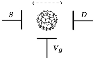
Figure 1: Schematic representation of tunneling between a source and a drain through a quantum dot. The dot is harmonically bound and vibrational motion can be excited as electrons tunnel through the system.

Boese and SchoellerBoese have recently given a theoretical description of the conductance features of this system. A more detailed analysis using similar techniques was given by Aji et al.Aji . Our objective is to extend these models to provide a full master equation description of the irreversible dynamics, including quantum correlation between the mechanical and electronic degrees of freedom. We wish to go beyond a rate equation description so as to be able to include coherent quantum effects which arise, for example, when the mechanical degree of freedom is subject to coherent driving.

II The model

We will assume that the center of mass of the dot is bound in a harmonic potential with resonant frequency $\omega_{o}$. This vibrational degree of freedom is then described by a displacement operator $\hat{x}$ which can be written in terms of annihilation and creation operators $a,a^{\dagger}$ as

$$\hat{x}=\sqrt{\frac{\hbar}{2m\omega_{o}}}(a+a^{\dagger}).$$ (1)

The electronic single quasi-bound state on the dot is described by Fermi annihilation and creation operators $c,c^{\dagger}$, which satisfy the anti commutation relation $cc^{\dagger}+c^{\dagger}c=1$.

The Hamiltonian of the system can then be written as,

$$H=\hbar\omega_{I}(V_{g})c^{\dagger}c+U_{c}\hat{n}^{2}$$ (7)

$$+\hskip 2.84544pt\hbar\omega_{o}a^{\dagger}a$$

$$+\hskip 2.84544pt\hbar\sum_{k}\omega_{Sk}a_{k}^{\dagger}a_{k}+\hbar\sum_{k}\omega_{Dk}b_{k}^{\dagger}b_{k}$$

$$-\chi(a^{\dagger}+a)\hat{n}$$

$$+\sum_{k}T_{Sk}(a_{k}c^{\dagger}+ca_{k}^{\dagger})+\sum_{k}T_{Dk}(b_{k}c^{\dagger}+cb_{k}^{\dagger})$$

$$+\sum_{p}\hbar\omega_{p}d_{p}^{\dagger}d_{p}+g_{p}(a^{\dagger}d_{p}+ad_{p}^{\dagger}),$$

where $\hat{n}=c^{\dagger}c$ is the excess electron number operator on the dot.

The first term of the Hamiltonian describes the free energy for the island. A particular gate voltage $V_{g}$, with a corresponding $\hbar\omega_{I}=15meV$, for the island is chosen for calculation. $U_{c}$ is the Coulomb charge energy which is the energy that is required to add an electron when there is already one electron occupying the island. We will assume this energy is large enough so that no more than one electron occupies the island at any time. This is a Coulomb Blockade effect. The charging energy of the fullerene molecule transistor has been observed by Park et al. to be larger than 270 meV which is two orders of magnitude larger than the vibrational quantum of energy $\hbar\omega_{o}$. The free Hamiltonian for the oscillator is described in term (7). The Park et al. experiment gives the value $\hbar\omega_{o}=5$ meV, corresponding to a THz oscillator. The electrostatic energy of electrons in the source and drain reservoirs is written as term (7). Term (7) is the coupling between the oscillator and charge while term (7) represents the source-island tunnel coupling and the drain-island tunnel coupling. The last term, (7), describes the coupling between the oscillator and the thermo-mechanical bath responsible for damping and thermal noise in the mechanical system in the rotating wave approximationGardiner-Zoller . This is an additional source of damping to that which can arise due to the transport process itself (see below). We include it in order to bound the motion under certain bias conditions. A possible physical origin of this source of dissipation will be discussed after the derivation of the master equation.

We have neglected the position dependence of the tunneling rate onto and off the island. This is equivalent to assuming that the distance, $d$, between the electrodes and the equilibrium position of the uncharged quantum dot, is much larger than the rms position fluctuations in the ground state of the oscillator. There are important situations where this approximation cannot be made, for example in the so called ‘charge shuttle’ systems shuttle-rev .

A primary difficulty in analyzing the quantum dynamics of this open system is the presence of different time scales associated with the oscillator, the tunneling events and the coupling between the oscillator and electronic degrees of degree due to the electrostatic potential, term (4). The standard approach would be to move to an interaction picture for the oscillator and the electronic degrees of freedom. However this would make the electrostatic coupling energy time dependent, and rapidly oscillating. Were we to approximate this with the secular terms stemming from a Dyson expansion of the Hamiltonian, the resulting effective coupling between the oscillator and the electron occupation of the dot simply shifts the free energy of the dot and no excitation of the mechanical motion can occur.

To avoid this problem we eliminate the coupling term of the oscillator and charge by doing a canonical transformation with unitary representation $U=e^{s}$ where,

$$s=-\lambda(a^{\dagger}-a)\hat{n}$$ (8)

with

$$\lambda=\frac{\chi}{\hbar\omega_{o}}\;.$$ (9)

This unitary transformation gives a conditional displacement of the oscillator conditional on the electronic occupation the dot. One might call this a displacement picture.

This derivation follows the approach of Mahan mahan . The motivation behind this is as follows. The electrostatic interaction, term (4), displaces the equilibrium position of the oscillator so that the average value of the oscillator amplitude in the ground state becomes

$$\langle a\rangle=\lambda,$$ (10)

We can shift this back to the origin by a phase-space displacement

$$\bar{a}\equiv e^{s}ae^{-s}=a+\lambda\hat{n}.$$ (11)

This unitary transformation gives a conditional displacement of the oscillator, conditional on the electronic occupation of the dot. Applying $U$ to the Fermi operator $c$ gives

$$\bar{c}=ce^{\lambda(a^{\dagger}-a)}.$$ (12)

The Schrödinger equation for the displaced state, $\bar{\rho}=e^{s}\rho e^{-s}$, then takes the form

$$\frac{d\bar{\rho}}{dt}=-\frac{i}{\hbar}[\bar{H},\bar{\rho}],$$ (13)

where the transformed Hamiltonian is

$$\bar{H}=\hbar\omega_{o}a^{\dagger}a+\hbar\omega_{I}(V_{g})c^{\dagger}c+\sum_{k}\hbar\omega_{Sk}a_{k}^{\dagger}a_{k}+\sum_{k}\hbar\omega_{Dk}b_{k}^{\dagger}b_{k}+(U_{c}+\frac{\chi^{2}}{\hbar\omega_{o}})\hat{n}^{2}$$

$$+\sum_{k}T_{Sk}\left(a_{k}c^{\dagger}e^{\lambda(a^{\dagger}-a)}+ca_{k}^{\dagger}e^{-\lambda(a^{\dagger}-a)}\right)$$

$$+\sum_{k}T_{Dk}\left(b_{k}c^{\dagger}e^{\lambda(a^{\dagger}-a)}+cb_{k}^{\dagger}e^{-\lambda(a^{\dagger}-a)}\right)\;.$$ (14)

We will now work exclusively in this displacement picture.

To derive a master equation for the dot, we first transform to an interaction picture in the usual way to give the Hamiltonian

$$H_{I} = \sum T_{Sk}(a_{k}c^{\dagger}e^{i(\omega_{I}-\eta-\omega_{Sk})t}e^{-\lambda(a^{\dagger}e^{i\omega_{o}t}-ae^{-i\omega_{o}t})}$$ (15)

$$\hskip 36.135pt+ca_{k}^{\dagger}e^{-i(\omega_{I}-\eta-\omega_{Sk})t}e^{\lambda(a^{\dagger}e^{i\omega_{o}t}-ae^{-i\omega_{o}t})})$$

$$+\sum T_{Dk}(b_{k}c^{\dagger}e^{i(\omega_{I}-\eta-\omega_{Dk})t}e^{-\lambda(a^{\dagger}e^{i\omega_{o}t}-ae^{-i\omega_{o}t})}$$

$$\hskip 36.135pt+cb_{k}^{\dagger}e^{-i(\omega_{I}-\eta-\omega_{Dk})t}e^{\lambda(a^{\dagger}e^{i\omega_{o}t}-ae^{-i\omega_{o}t})}),$$

where $\eta={\chi^{2}}/({\hbar\omega_{o}})=\chi\lambda$.

At this point we might wish to trace out the phonon bath, however we will postpone this for a closer look at the tunneling Hamiltonian at the individual phonon level. We use the exponential approximation $e^{x}=1+x+x^{2}/(2!)+\cdots$ , when $x$ is small for the term $e^{\lambda(a^{\dagger}e^{i\omega_{o}t}-ae^{-i\omega_{o}t})}$. We expect an expansion to second order in $\lambda$ to give an adequate description of transport, in that at least one step in the current vs. bias voltage curve is seen due to phonon mediated tunneling. In the experiment of Park et al., $\lambda$ was less than unity, but not very small. Strong coupling between the electronic and vibrational degrees of freedom (large $\lambda$) will give multi-phonon tunneling events, and corresponding multiple steps in the current vs. bias voltage curves. The Hamiltonian can then be written as

$$H_{I} = \sum T_{Sk}(a_{k}c^{\dagger}e^{i(\omega_{I}-\eta-\omega_{Sk})t}+ca_{k}^{\dagger}e^{-i(\omega_{I}-\eta-\omega_{Sk})t})$$ (16)

$$+\lambda\sum T_{Sk}(a_{k}c^{\dagger}ae^{i(\omega_{I}-\eta-\omega_{Sk}-\omega_{o})t}+ca_{k}^{\dagger}a^{\dagger}e^{-i(\omega_{I}-\eta-\omega_{Sk}-\omega_{o})t}$$

$$\hskip 36.135pt-a_{k}c^{\dagger}a^{\dagger}e^{i(\omega_{I}-\eta-\omega_{Sk}+\omega_{o})t}-ca_{k}^{\dagger}ae^{-i(\omega_{I}-\eta-\omega_{Sk}+\omega_{o})t})$$

$$+\frac{\lambda^{2}}{2}\sum T_{Sk}(a_{k}c^{\dagger}aae^{i(\omega_{I}-\eta-\omega_{Sk}-2\omega_{o})t}+ca_{k}^{\dagger}a^{\dagger}a^{\dagger}e^{-i(\omega_{I}-\eta-\omega_{Sk}-2\omega_{o})t}$$

$$\hskip 36.135pt-2a_{k}c^{\dagger}a^{\dagger}ae^{i(\omega_{I}-\eta-\omega_{Sk})t}-2ca_{k}^{\dagger}a^{\dagger}ae^{-i(\omega_{I}-\eta-\omega_{Sk})t}$$

$$\hskip 36.135pt+a_{k}c^{\dagger}a^{\dagger}a^{\dagger}e^{i(\omega_{I}-\eta-\omega_{Sk}+2\omega_{o})t}-ca_{k}^{\dagger}aae^{-i(\omega_{I}-\eta-\omega_{Sk}+2\omega_{o})t})$$

$$+\sum T_{Dk}(b_{k}c^{\dagger}e^{i(\omega_{I}-\eta-\omega_{Dk})t}+cb_{k}^{\dagger}e^{-i(\omega_{I}-\eta-\omega_{Dk})t})$$

$$+\lambda\sum T_{Dk}(-b_{k}c^{\dagger}a^{\dagger}e^{i(\omega_{I}-\eta-\omega_{Dk}+\omega_{o})t}-cb_{k}^{\dagger}ae^{-i(\omega_{I}-\eta-\omega_{Dk}+\omega_{o})t}$$

$$\hskip 36.135pt+b_{k}c^{\dagger}ae^{i(\omega_{I}-\eta-\omega_{Dk}-\omega_{o})t}+cb_{k}^{\dagger}a^{\dagger}e^{-i(\omega_{I}-\eta-\omega_{Dk}-\omega_{o})t})$$

$$+\frac{\lambda^{2}}{2}\sum T_{Dk}(b_{k}c^{\dagger}aae^{i(\omega_{I}-\eta-\omega_{Dk}-2\omega_{o})t}+cb_{k}^{\dagger}a^{\dagger}a^{\dagger}e^{-i(\omega_{I}-\eta-\omega_{Dk}-2\omega_{o})t}$$

$$\hskip 36.135pt-2b_{k}c^{\dagger}a^{\dagger}ae^{i(\omega_{I}-\eta-\omega_{Dk})t}-2cb_{k}^{\dagger}a^{\dagger}ae^{-i(\omega_{I}-\eta-\omega_{Dk})t}$$

$$\hskip 36.135pt+b_{k}c^{\dagger}a^{\dagger}a^{\dagger}e^{i(\omega_{I}-\eta-\omega_{Dk}+2\omega_{o})t}-cb_{k}^{\dagger}aae^{-i(\omega_{I}-\eta-\omega_{Dk}+2\omega_{o})t}).$$

The terms of zero order in $\lambda$ describe bare tunneling through the system and do not cause excitations of the vibrational degree of freedom. The terms linear in $\lambda$ correspond to the exchange of one vibrational quantum, or phonon. The terms quadratic in $\lambda$ correspond to tunneling with the exchange of two vibrational quanta. Higher order terms could obviously be included at considerable computational expense. We will proceed to derive the master equation up to quadratic order in $\lambda$.

III Master equation

Our objective here is to find an evolution equation of the joint density operator for the electronic and vibrational degrees of freedom. We will use standard methods based on the Born and Markov approximationGardiner-Zoller . In order to indicate where these approximations occur, we will sketch some of the key elements of the derivation in what follows. The Born approximation assumes that the coupling between the leads and the local system is weak and thus second order perturbation theory will suffice to describe this interaction;

$$\dot{\rho} = \frac{-1}{\hbar^{2}}\int_{0}^{t}dt^{\prime}\rm{Tr}[H_{I}(t),[H_{I}(t^{\prime}),R]],$$ (17)

where $R$ is the joint density matrix for the vibrational and electronic degrees of freedom of the local system and the reservoirs.

At this point we would like to trace out the electronic degrees of freedom for the source and drain. We will assume that the states of the source and drain remain in local thermodynamic equilibrium at temperature $T$. This is part of the Markov approximation. Its validity requires that any correlation that develops between the electrons in the leads and the local system, as a result of the tunneling interaction, is rapidly damped to zero on time scales relevant for the system dynamics. We need the following moments:

$${\rm Tr}[a_{k}^{\dagger}a_{k}\rho]=f_{Sk},\hskip 56.9055pt {\rm Tr}[b_{k}^{\dagger}b_{k}\rho]=f_{Dk},$$

$${\rm Tr}[a_{k}a_{k}^{\dagger}\rho]=1-f_{Sk},\hskip 56.9055pt {\rm Tr}[b_{k}b_{k}^{\dagger}\rho]=1-f_{Dk}.$$

where $f_{Sk}=f(E_{Sk})$ is the Fermi function describing the average occupation number in the source and similarly $f_{Dk}=f(E_{Dk})$, for the drain. The Fermi function has an implicit dependence on the temperature, $T$, of the electronic system.

The next step is to convert the sum over modes to a frequency-space integral:

$$\sum_{k}f_{Sk}|T_{Sk}|^{2}\rightarrow\int_{0}^{\infty}d\omega\hskip 2.84526ptg(\omega)f_{D}(\omega)|T_{S}(\omega)|^{2},$$ (18)

where $|T_{Sk}|^{2}=T_{Sk}^{*}T_{Sk}$ and $g(\omega)$ is the density of states. Evaluating the time integral, we use,

$$\int_{0}^{\infty}d\tau e^{\pm i\epsilon\tau}=\pi\delta(\epsilon)\pm iPV(1/\epsilon),$$ (19)

where $\tau=t-t^{\prime}$ and the imaginary term is ignored.

Using these methods, we can combine the terms for the source and drain as the left and right tunneling rates, $\gamma_{L}$ and $\gamma_{R}$ respectively

$$\int_{0}^{\infty}d\omega\hskip 2.84526ptg(\omega)|T_{S}(\omega)|^{2}\delta(\omega_{0})=\gamma_{L}(\omega_{0}).$$ (20)

In the same way, we can define

$$\gamma_{L1} = \gamma_{L}(\hbar\omega_{I}-\eta-\mu_{L}),$$

$$f_{1L} = f(\hbar\omega_{I}-\eta-\mu_{L}),$$

$$\gamma_{L2} = \gamma_{L}(\hbar\omega_{I}-\eta-\hbar\omega_{o}-\mu_{L}),$$

$$f_{2L} = f(\hbar\omega_{I}-\eta-\hbar\omega_{o}-\mu_{L}),$$

$$\gamma_{L3} = \gamma_{L}(\hbar\omega_{I}-\eta+\hbar\omega_{o}-\mu_{L}),$$

$$f_{3L} = f(\hbar\omega_{I}-\eta+\hbar\omega_{o}-\mu_{L}).$$

and similarly for $\gamma_{R1},\gamma_{R2}\gamma_{R3},f_{1R},f_{2R},f_{3R}$ replacing $\mu_{L}$ with $\mu_{R}$ and $f$ being the Fermi functions which have a dependence on the bias voltage (through the chemical potential) and also on the phonon energy $\hbar\omega_{o}$. As the bias voltage is increased from zero, the first Fermi function to be significantly different from zero is $f_{2L}$ followed by $f_{1L}$ and then $f_{3L}$. This stepwise behavior will be important in understanding the dependence of the stationary current as a function of bias voltage.

The master equation in the canonical transformed picture to the second order in $\lambda$ may be written as

$$\frac{d\bar{\rho}}{dt} = \gamma_{L1}\biggl{(}(1-\lambda^{2})(f_{1L}\mathcal{D}[c^{\dagger}]\bar{\rho}+(1-f_{1L})\mathcal{D}[c]\bar{\rho})$$ (21)

$$\hskip 21.68121pt+\lambda^{2}\ (f_{1L}(-a^{\dagger}ac^{\dagger}\bar{\rho}c+a^{\dagger}acc^{\dagger}\bar{\rho}-c^{\dagger}\bar{\rho}ca^{\dagger}a+\bar{\rho}cc^{\dagger}a^{\dagger}a)$$

$$\hskip 36.135pt+(1-f_{1L})(-a^{\dagger}ac\bar{\rho}c^{\dagger}+a^{\dagger}ac^{\dagger}c\bar{\rho}-c\bar{\rho}c^{\dagger}a^{\dagger}a+\bar{\rho}a^{\dagger}ac^{\dagger}c))\biggr{)}$$

$$+ \gamma_{L2}\lambda^{2}\biggl{(}f_{2L}\mathcal{D}[ac^{\dagger}]\bar{\rho}+(1-f_{2L})\mathcal{D}[a^{\dagger}c]\bar{\rho}\biggr{)}$$

$$+ \gamma_{L3}\lambda^{2}\biggl{(}f_{3L}\mathcal{D}[a^{\dagger}c^{\dagger}]\bar{\rho}+(1-f_{3L})\mathcal{D}[ac]\bar{\rho}\biggr{)}$$

$$+ \gamma_{R1}\biggl{(}(1-\lambda^{2})(f_{1R}\mathcal{D}[c^{\dagger}]\bar{\rho}+(1-f_{1R})\mathcal{D}[c]\bar{\rho})$$

$$\hskip 21.68121pt+\lambda^{2}\ (f_{1R}(-a^{\dagger}ac^{\dagger}\bar{\rho}c+a^{\dagger}acc^{\dagger}\bar{\rho}-c^{\dagger}\bar{\rho}ca^{\dagger}a+\bar{\rho}cc^{\dagger}a^{\dagger}a)$$

$$\hskip 36.135pt+(1-f_{1R})(-a^{\dagger}ac\bar{\rho}c^{\dagger}+a^{\dagger}ac^{\dagger}c\bar{\rho}-c\bar{\rho}c^{\dagger}a^{\dagger}a+\bar{\rho}a^{\dagger}ac^{\dagger}c))\biggr{)}$$

$$+ \gamma_{R2}\lambda^{2}\biggl{(}f_{2R}\mathcal{D}[ac^{\dagger}]\bar{\rho}+(1-f_{2R})\mathcal{D}[a^{\dagger}c]\bar{\rho}\biggr{)}$$

$$+ \gamma_{R3}\lambda^{2}\biggl{(}f_{3R}\mathcal{D}[a^{\dagger}c^{\dagger}]\bar{\rho}+(1-f_{3R})\mathcal{D}[ac]\bar{\rho}\biggr{)}$$

$$+ \kappa(\bar{n}_{p}+1)\mathcal{D}[a]\bar{\rho}+\kappa\bar{n}_{p}\mathcal{D}[a^{\dagger}]\bar{\rho}+\kappa\lambda^{2}(2\bar{n}_{p}+1)\mathcal{D}[c^{\dagger}c]\bar{\rho}\;,$$

where the notation ${\cal D}$ is defined for arbitrary operators $X$ and $Y$ as

$$\mathcal{D}[X]Y = \mathcal{J}[X]Y-\mathcal{A}[Y]$$ (22)

$$= XYX^{\dagger}-\frac{1}{2}(X^{\dagger}XY+YX^{\dagger}X),$$

and

$$\bar{n}_{p}(\omega_{o})=\frac{1}{e^{\hbar\omega_{o}/k_{B}T}-1}\;.$$ (23)

We have included in this model an explicit damping process of the oscillators motion at rate $\kappa$ into a thermal oscillator bath with mean excitation $\bar{n}_{p}$ and $T$ is the effective temperature of reservoir responsible for this damping process. A possible physical origin for this kind of damping could be as follows. Thermal fluctuations in the metal contacts of the source and drain cause fluctuations in position of the center of the trapping potential confining the molecule, that is to say small, fluctuating linear forces act on the molecule. For a harmonic trap, this appears to the oscillator as a thermal bath. However we expect such a mechanism to be very weak. This fact, together with the very large frequency of the oscillator, justifies our use of the quantum optical master equation (as opposed to the Brownian motion master equation) to describe this source of dissipationGardiner-Zoller . The thermo-mechanical and electronic temperatures are not necessarily the same, although we will generally assume this to be the case.

Setting $\lambda=0$ we recover the standard master equation for a single quantum dot coupled to leadsSun . The superoperator ${\cal D}[c^{\dagger}]$ adds one electron to the dot. Terms containing this super operator describe a conditional Poisson event in which an electron tunnels onto the dot. The electron can enter from the source, with probability per unit time of $\gamma_{L1}f_{1L}\langle cc^{\dagger}\rangle$, or it can enter from the drain, with probability per unit time $\gamma_{R1}f_{1R}\langle cc^{\dagger}\rangle$. Likewise the term ${\cal D}[c]$ describes an electron leaving the dot, again via tunneling into the source (terms proportional to $\gamma_{L1}$) or the drain (terms proportional to $\gamma_{R1}$). When $\lambda\neq 0$ there are additional terms describing phonon mediated tunneling events onto and off the dot. Any term proportional to $\gamma_{Li},\ i=1,2,3.$ describes an electron tunneling out of, or into, the source, while any term proportional to $\gamma_{Ri},\ i=1,2,3$ describes an electron tunneling out of, or into, the drain.

The average currents through the left junction (source lead–dot) and the right junction (dot–drain lead) are related to each other, and the average occupation of the dot, by

$$I_{L}(t)-I_{R}(t)=e\frac{d\langle c^{\dagger}c\rangle}{dt}.$$ (24)

In the steady state, the occupation of the dot is constant and the average currents through the two junctions are equal. Of course, the actual fluctuating time dependent currents are almost never equal. The external current arises as the external circuit adjusts the chemical potential of the local Fermi reservoir when electrons tunnel onto or off the dot. It is thus clear that the current through the left junction must depend only on the tunneling rates $\gamma_{Li},\ i=1,2,3.$ in the left barrier. This makes it easy to identify the average current through the left (or right) junction by inspection of the equation of motion for $\langle c^{\dagger}c\rangle$: all terms in the right hand side of Eq. (24) proportional to $\gamma_{Li}$ correspond to the average current through the left junction, $I_{L}(t)$, while all terms on the right hand side proportional to $\gamma_{Ri}$ correspond to the negative of the current through the right junction, $-I_{R}(t)$.

IV Local system dynamics

We can now compute the current through the quantum dot. The current reflects how the reservoirs of the source and drain respond to the dynamics of the vibrational and electronic degrees of freedom. Of course in an experiment the external current is typically all we have access to. However the master equation enables us to calculate the coupled dynamics of the vibrational and electronic degrees of freedom. Understanding this dynamics is crucial to explaining the observed features in the external current. As electrons tunnel on and off the dot, the oscillator experiences a force due to the electrostatic potential. While the force is conservative, the tunnel events are stochastic (in fact a Poisson process) and thus the excitation of the oscillator is stochastic. Furthermore the vibrational and electronic degrees of freedom become correlated through the dynamics. In this section we wish to investigate these features in some detail.

From the master equation, the rate of change of this average electron number in the dot may be obtained:

$$\frac{d\langle c^{\dagger}c\rangle_{\rm CT}}{dt} = {\rm tr}[c^{\dagger}c\frac{d\bar{\rho}}{dt}]$$ (26)

$$= [\gamma_{L1}(1-\lambda^{2})(f_{1L}-\langle c^{\dagger}c\rangle)+\gamma_{R1}(1-\lambda^{2})(f_{1R}-\langle c^{\dagger}c\rangle)$$

$$-2\gamma_{L1}\lambda^{2}(f_{1L}\langle a^{\dagger}a\rangle-\langle a^{\dagger}ac^{\dagger}c\rangle)$$

$$+\gamma_{L2}\lambda^{2}(f_{2L}\langle a^{\dagger}a\rangle-\langle a^{\dagger}ac^{\dagger}c\rangle-(1-f_{2L})\langle c^{\dagger}c\rangle)$$

$$+\gamma_{L3}\lambda^{2}(f_{3L}\langle 1+a^{\dagger}a\rangle-f_{3L}\langle c^{\dagger}c\rangle-\langle a^{\dagger}ac^{\dagger}c\rangle)$$

$$-2\gamma_{R1}\lambda^{2}(f_{1R}\langle a^{\dagger}a\rangle-\langle a^{\dagger}ac^{\dagger}c\rangle)$$

$$+\gamma_{R2}\lambda^{2}(f_{2R}\langle a^{\dagger}a\rangle-\langle a^{\dagger}ac^{\dagger}c\rangle-(1-f_{2R})\langle c^{\dagger}c\rangle)$$

$$+\gamma_{R3}\lambda^{2}(f_{3R}\langle 1+a^{\dagger}a\rangle-f_{3R}\langle c^{\dagger}c\rangle-\langle a^{\dagger}ac^{\dagger}c\rangle)]_{\rm CT}\ .$$

While for the vibrational degrees of freedom, we see that

$$\frac{d\langle a^{\dagger}a\rangle_{\rm CT}}{dt} = {\rm tr}[a^{\dagger}a\frac{d\bar{\rho}}{dt}]$$ (28)

$$= \lambda^{2}[\gamma_{L2}(-f_{2L}\langle a^{\dagger}a\rangle+\langle a^{\dagger}ac^{\dagger}c\rangle+(1-f_{2L})\langle c^{\dagger}c\rangle)$$

$$+\gamma_{L3}(f_{3L}\langle 1+a^{\dagger}a\rangle-f_{3L}\langle c^{\dagger}c\rangle-\langle a^{\dagger}ac^{\dagger}c\rangle)$$

$$+\gamma_{R2}(-f_{2R}\langle a^{\dagger}a\rangle+\langle a^{\dagger}ac^{\dagger}c\rangle+(1-f_{2R})\langle c^{\dagger}c\rangle)$$

$$+\gamma_{R3}(f_{3R}\langle 1+a^{\dagger}a\rangle-f_{3R}\langle c^{\dagger}c\rangle-\langle a^{\dagger}ac^{\dagger}c\rangle)-\kappa\langle a^{\dagger}a\rangle]_{\rm CT}+\kappa\bar{n}_{p}\ .$$

Here the subscript CT indicates that the quantity to which it is attached is evaluated in the canonical transformed (CT) basis. The average occupational number of electron in the dot in the original basis is the same as in the CT basis:

$$\langle c^{\dagger}c\rangle={\rm tr}[c^{\dagger}c\rho]={\rm tr}[c^{\dagger}c\bar{\rho}]=\langle c^{\dagger}c\rangle_{\rm CT}.$$

While for the vibrational degrees of freedom, we have

$$\langle a^{\dagger}a\rangle = {\rm tr}[a^{\dagger}a\rho]$$ (29)

$$= {\rm tr}[a^{\dagger}ae^{-s}e^{-i\omega_{o}a^{\dagger}at}\bar{\rho}e^{i\omega_{o}a^{\dagger}at}e^{s}]$$

$$= {\rm tr}[e^{i\omega_{o}a^{\dagger}at}(a^{\dagger}+\lambda\hat{n})(a+\lambda\hat{n})e^{-i\omega_{o}a^{\dagger}at}\bar{\rho}]$$

$$= \langle a^{\dagger}a\rangle_{\rm CT}+\lambda\langle(a^{\dagger}e^{-i\omega_{o}a^{\dagger}at}+ae^{-i\omega_{o}a^{\dagger}at})\hat{n}\rangle_{\rm CT}+\lambda^{2}\langle\hat{n}^{2}\rangle.$$

If the initial displacement $\langle x\rangle$ is zero, the second time dependent term in the previous expression remains zero. We will assume this is the case in what follows.

In general we do not get a closed set of equations for the mean phonon and electron number due to the presence in these equations of the higher order moment $\langle a^{\dagger}ac^{\dagger}c\rangle$. This reflects the fact that the electron and vibrational degrees of freedom are correlated (and possibly entangled) through the dynamics. One might proceed by introducing a semiclassical factorization approximation by replacing $\langle a^{\dagger}ac^{\dagger}c\rangle$ by the factorized average values, i.e., $\langle a^{\dagger}ac^{\dagger}c\rangle\approx\langle a^{\dagger}a\rangle\langle c^{\dagger}c\rangle$, then the evolution equations (26) and (28) forms a closed set of equations. However there is a special case for which this is not necessary. If we let $\gamma_{L1}=\gamma_{L2}=\gamma_{L3}=\gamma_{L}$ and $\gamma_{R1}=\gamma_{R2}=\gamma_{R3}=\gamma_{R}$ which is the assumption of energy-independent tunnel couplings, the equations do form a closed set:

$$\frac{d\langle c^{\dagger}c\rangle}{dt} = A_{1}\langle c^{\dagger}c\rangle+B_{1}\langle a^{\dagger}a\rangle_{\rm CT}+C_{1}\;,$$ (30)

$$A_{1} = -\bigl{[}\gamma_{L}(1-f_{2L}\lambda^{2}+f_{3L}\lambda^{2})+\gamma_{R}(1-f_{2R}\lambda^{2}+f_{3R}\lambda^{2})\bigr{]},$$

$$B_{1} = \lambda^{2}(-2f_{1L}\gamma_{L}+f_{2L}\gamma_{L}+f_{3L}\gamma_{L}-2f_{1R}\gamma_{R}+f_{2R}\gamma_{R}+f_{3R}\gamma_{R}),$$

$$C_{1} = (1-\lambda^{2})\gamma_{L}f_{1L}+\gamma_{L}f_{3L}\lambda^{2}+(1-\lambda^{2})\gamma_{R}f_{1R}+\gamma_{R}f_{3R}\lambda^{2}\;,$$

and

$$\frac{d\langle a^{\dagger}a\rangle_{\rm CT}}{dt} = A_{2}\langle c^{\dagger}c\rangle+B_{2}\langle a^{\dagger}a\rangle_{\rm CT}+C_{2}\;,$$ (31)

$$A_{2} = \lambda^{2}(\gamma_{L}(1-f_{2L}-f_{3L})+\gamma_{R}(1-f_{2R}-f_{3R})),$$

$$B_{2} = \lambda^{2}(-\gamma_{L}f_{2L}+\gamma_{L}f_{3L}-\gamma_{R}f_{2R}+\gamma_{R}f_{3R})-\kappa,$$

$$C_{2} = \lambda^{2}(\gamma_{L}f_{3L}+\gamma_{R}f_{3R})+\kappa\bar{n}_{p}\;.$$

Consideration of Eq. (31) indicates that it is possible for the oscillator to achieve a steady state even when there is no explicit thermo-mechanical damping ($\kappa=0$). This requires bias conditions such that $f_{3L}=f_{3R}=0$. It is remarkable that the process of electrical transport between source and drain alone can induce damping of the mechanical motion. This result has been indicated by other authorsMozyrsky-Martin ; Smirnov ; Mozyrsky-Martin-Hastings ; Armour .

These equations were solved numerically and the results, for various values of $\lambda$ and bias voltage, are shown in Fig. 2. A feature of our approach is that we can directly calculate the dynamics of the local degrees of freedom, for example the mean electron occupation of the dot as well as the mean vibrational occupation number in the oscillator.

From these equations we can reproduce behavior for the stationary current similar to that observed in the experiment. We concentrate here on the stationary current through the left junction (connected to the source). Similar results apply for the right junction. We assume that the electronic temperature is $1.5$K, which is the temperature used in the experiment by Park et al. Park .

Following the discussion below Eq. (24), we see from Eq. (30) that the average steady state current through the left junction is given by

$$I_{\rm st} = e\gamma_{L}[(-1+f_{2L}\lambda^{2}-f_{3L}\lambda^{2})\langle c^{\dagger}c\rangle_{\rm st}+(-2f_{1L}\lambda^{2}+f_{2L}\lambda^{2}+f_{3L}\lambda^{2})\langle a^{\dagger}a\rangle_{\rm CT,st}$$ (32)

$$+(1-\lambda^{2})f_{1L}+f_{3L}\lambda^{2}].$$

which is of course equal to the average steady state current through the right junction. The steady state current, $I_{\rm st}$ can then be found by finding the steady state solution for each of the phonon number and electron number,

$$\langle c^{\dagger}c\rangle_{\rm st} = \frac{B_{1}C_{2}-B_{2}C_{1}}{A_{1}B_{2}-A_{2}B_{1}}\;,$$ (33)

$$\langle a^{\dagger}a\rangle_{\rm CT,st} = \frac{-A_{2}}{B_{2}}\biggl{(}\frac{B_{1}C_{2}-B_{2}C_{1}}{A_{1}B_{2}-A_{2}B_{1}}\biggr{)}-\frac{C_{2}}{B_{2}}\;.$$ (34)

In Fig. 2, we assume that the bias voltage is applied symmetrically, i.e, $\mu_{L}=-\mu_{R}=eV_{\rm bias}/2$. In this case, all the Fermi factors $f_{1R}$, $f_{2R}$, and $f_{3R}$ effectively equal to zero in the positive bias regime, the regime of Fig. 2. From Eqs. (24) and (30), we see that Eq. (32) also equals to the steady state current through the right junction as: $I_{\rm st}=e\gamma_{R}\langle c^{\dagger}c\rangle_{\rm st}$. In the case $\gamma_{R}=\gamma_{L}$, the steady state $\langle c^{\dagger}c\rangle_{\rm st}$ shown in Fig. 2(a) and (d) at long times should thus equal respectively to $I_{\rm st}/(e\gamma_{L})$ shown in Fig. 2(c) and (f) at long times. This is indeed the case, although the transient behaviors in these plots differ considerably. We note that the plot shown in Fig. 2(c) and (f) is the current through the left junction, normalized by $(e\gamma_{L})$. The values of $f_{1L}$, $f_{2L}$, and $f_{3L}$ depend on the strength of the applied bias voltage and are important in understanding the stepwise behavior of the stationary current as a function of the bias voltage. We will now concentrate exclusively on the positive bias regime.

When the bias voltage is small, the current is zero. As the bias voltage increases the first Fermi factor in the left lead to become non zero is $f_{2L}$, with the other Fermi factors very small or zero. In the case that $f_{2L}=1,\ f_{1L}=0,\ f_{3L}=0$, the steady state current is

$$I^{(1)}_{\rm st}=e\gamma_{L}[\lambda^{2}\langle a^{\dagger}a\rangle_{\rm CT,st}-(1-\lambda^{2})\langle c^{\dagger}c\rangle_{\rm st}]\ ,$$ (35)

For low temperatures this is very small. Only if the phonon temperature is large, so that the stationary mean phonon number is significant, does this first current step become apparent (see Fig. 4). As the bias voltage is increased both $f_{2L}$ and $f_{1L}$ become non zero. In the case where they are both unity, the steady state current is

$$I^{(2)}_{\rm st}=e\gamma_{L}[(1-\lambda^{2})\langle cc^{\dagger}\rangle_{\rm st}-\lambda^{2}\langle a^{\dagger}a\rangle_{\rm CT,st}]\ .$$ (36)

The first term here is the same form as the bare tunneling case except that the effective tunneling rate is reduced by $(1-\lambda^{2})$. This is not too surprising. If the island is moving, on average it reduces the effective tunneling rate across the two barriers. Thus the first current step will be reduced below the value of the bare (no phonon) rate. At the region where bias voltage is large, all the Fermi factors are unity and

$$I^{(3)}_{\rm st}=e\gamma_{L}\langle cc^{\dagger}\rangle_{st}\;,$$ (37)

which is the expected result for the bare tunneling case.

To explicitly evaluate the stationary current we need to solve for the stationary mean electronic and phonon occupation numbers. We have done this numerically and the results are shown in the figures below. However the large bias case can be easily solved;

$$\langle c^{\dagger}c\rangle_{\rm st} = \frac{\gamma_{L}}{\gamma_{L}+\gamma_{R}}\;,$$ (38)

$$\langle a^{\dagger}a\rangle_{\rm st} = \biggl{(}\lambda^{2}+\frac{\lambda^{2}(-\gamma_{L}+\gamma_{R})}{\kappa}\biggr{)}\biggl{(}\frac{\gamma_{L}}{\gamma_{L}+\gamma_{R}}\biggr{)}+\frac{\gamma_{L}\lambda^{2}+\kappa\bar{n}_{p}}{\kappa}\;,$$ (39)

$$I_{\rm st} = e\frac{\gamma_{L}\gamma_{R}}{\gamma_{L}+\gamma_{R}}\;.$$ (40)

This is the result for tunneling through a single quasi bound state between two barriers Sun .

The steady state current for larger values of $\lambda$ shows two steps. As one can see from Fig. 2(a), the current vanishes until the first Coulomb Blockade energy is overcome. The first step in the stationary current is thus due to bare tunneling though the dot. The second step represents single phonon mediated tunneling through the dot. These results are consistent with the semiclassical theory of Boese and SchoellerBoese given that our expansion to second order in $\lambda$ can only account for single phonon events. The height of the step depends on $\lambda$ which is the ratio of the coupling strength between the electron and the vibrational level $\chi$, and the oscillator energy $\hbar\omega_{o}$.

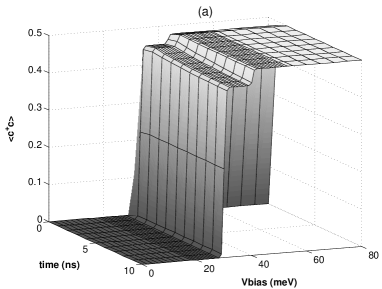
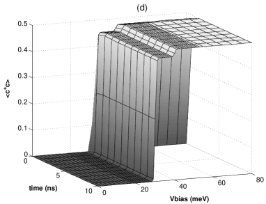
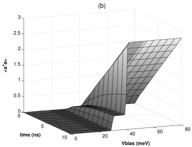
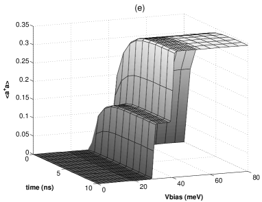
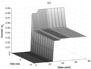
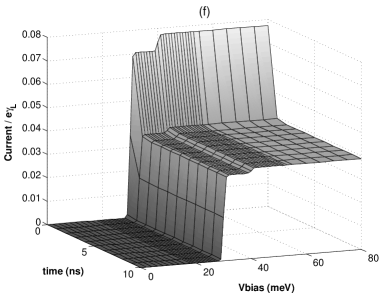
Figure 2: Average number of electron, phonon and current through the dot against bias voltage with $\hbar\omega_{o}=$ 5 meV, $\hbar\omega_{I}-\eta$ = 15 meV, $k_{B}T=$ 0.13 meV, and $\hbar\gamma_{L}=\hbar\gamma_{R}=$ 2 $\mu$eV for $\lambda=0.3$. Figures (a),(b),(c) without damping and (d),(e),(f) with damping $\kappa=0.3\gamma_{L}$. We assume $\mu_{L}=-\mu_{R}=eV_{\rm bias}/2$.

Looking at Fig. 2, the average electron number approaches a steady state (e.g., a steady state value of $0.5$ at large bias since we have set the value of $\gamma_{L}$ to be equal to $\gamma_{R}$) while the average phonon number, without external damping, behaves differently in various regions (Fig. 2(b)). The average phonon number slowly reaches a steady state value within the first step, while at the second step, the mean phonon number grows linearly with time (Fig. 2(b)). The steady state at the first step is the previously noted effect of transport induced damping. These results are as expected since from Eq. (21), the term consisting $\gamma_{L2}\lambda^{2}f_{2L}{\cal D}[ac^{\dagger}]\rho$ corresponds to a jump of one electron onto the island with the simultaneous annihilation of a phonon, while $\gamma_{L3}\lambda^{2}f_{3L}{\cal D}[a^{\dagger}c^{\dagger}]\rho$ corresponds to the jump of an electron onto the island along with the simultaneous creation of a phonon. The dynamics can be understood by relating the behavior of these terms to the rate of average phonon number change in Eq. (31). At the first step, when both $f_{1L}$ and $f_{2L}$ are both one, while $f_{3L}$ is zero, the coefficient $B_{2}$ has negative value, and therefore the mean phonon number could reach a steady state under this transport induced damping. In this regime, we find that

$$\langle c^{\dagger}c\rangle_{\rm st} = (1-\lambda^{2})/2\;,$$ (41)

$$\langle a^{\dagger}a\rangle_{\rm st} \approx 1/2\;,$$ (42)

where we have set $\gamma_{L}=\gamma_{R}$ and used Eq. (29) in obtaining Eq. (42). The corresponding effective temperature can be found using

$$T_{\rm eff}=\frac{\hbar\omega_{o}}{k_{B}\ln[1+(1/\langle a^{\dagger}a\rangle_{\rm st})]}\;.$$ (43)

When all the Fermi factors for the left lead are unity, the rate of growth for the mean phonon number now depends on a constant $C_{2}$ in Eq. (31) and therefore the mean phonon number will grow linearly with time. However, the current will be still steady (Fig. 2(f)). This indicates that the steady state current and mean electron number in the dot [given by Eqs. (40) and (38) respectively] do not depend on the mean phonon number. This is supported by the fact that the coefficient $B_{1}$ in Eq. (30) vanishes in this regime. When damping is included, the phonon number reaches a steady value of 0.35 [see Fig. 2(e) and also Eq. (39)].

In Fig. 3 we plot the steady state current versus bias voltage for different values of $\lambda$. At the region of the first phonon excitation level (when bias voltage is between 30 meV and 40 meV), the steady state current drops by a factor proportional to quadratic order of $\lambda$. Compared to the current at large bias voltage, the size of the drop is

$$\Delta I_{\rm st}=\frac{\gamma_{L}\lambda^{2}(2\gamma_{L}\lambda^{2}+\kappa(2\bar{n}_{p}+1))}{4\gamma_{L}\lambda^{2}-2\kappa(\lambda^{2}-2)}.$$ (44)

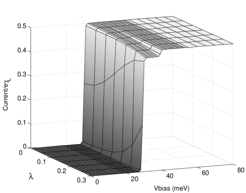
Figure 3: Steady state current for different values of $\lambda$ with damping $\kappa=0.3\gamma_{L}$, the electronic and phonon temperatures are both $1.5$K.

We thus see that the effect of the oscillatory motion of the island is two fold. Firstly the vibrational motion leads to an effective reduction in the tunneling rate by an amount $\lambda^{2}$ to lowest order in $\lambda$. Secondly there is a second step at higher bias voltage due to phonon mediated tunneling. This is determined by the dependence of the Fermi factors on the vibrational quantum of energy. One might have expected another step at a smaller bias voltage. However this step is very small unless there is a significant thermally excited mean phonon number present in the steady state. If we increase the phonon temperature such that the energy is larger than the energy quantum of the oscillator, $\hbar\omega_{o}$, (for this example we choose $T=2\hbar\omega_{o}/k_{B}\approx 116K$ ) this step can be seen (Fig 4). Thus we see three steps as expected, corresponding to the three bias voltages when the three Fermi factors switch from zero.

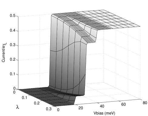
Figure 4: Steady state current for different values of $\lambda$ and damping $\kappa=0.3\gamma_{L}$, the electronic temperature is $1.5$K, and the phonon temperature is $116$K which is chosen to be $2\hbar\omega_{o}/k_{B}$ in order to make manifest the step at a smaller bias voltage.

In order to explore the steady state correlation between phonon number and electron number on the dot, we can find the steady state directly by solving the master equation from Eq. (21). In Fig. 5 we plot the correlation function $\langle a^{\dagger}ac^{\dagger}c\rangle-\langle a^{\dagger}a\rangle\langle c^{\dagger}c\rangle$ as a function of $\lambda$ and the bias voltage. The correlation is seen to be small except when a transition occurs between two conductance states. This is not surprising, as at this point one expects fluctuations in the charge on the dot, and consequently the fluctuations of phonon number, to be large. This interpretation implies that damping of the oscillator should suppress the correlation, as the response of the oscillator to fluctuations in the dot occupation are suppressed. This is seen in Fig. 6.

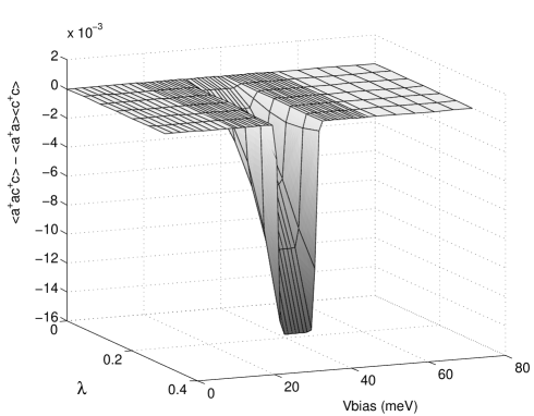
Figure 5: Difference in the correlation function for different values of $\lambda$ with damping $\kappa=0.3\gamma_{L}$.

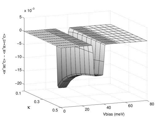
Figure 6: Difference in the correlation function for different values of $\kappa$ with damping $\lambda=0.3\gamma_{L}$. The plot starts at a value $\kappa\neq 0$.

V Conclusions

We have given a quantum description of a QEMS comprising a single quantum dot harmonically bound between two electrodes based on a quantum master equation for the density operator of the electronic and vibrational degrees of freedom. The description thus incorporates the dynamics of both diagonal (population) and off-diagonal (coherence) terms. We found a special set of parameters for which the equations of motion for the mean phonon number and the electron number form a closed set. From this we have been able to reproduce the central qualitative features of the current vs. bias voltage curve obtained experimentally by Park et al.Park and also of the semiclassical phenomenological theory by Boese and Schoeller Boese . We also calculate the correlation function between phonon and electron number in the steady state and find that it is only significant at the steps of the the steady state conductance. The results reported in this paper do not probe the full power of the master equation approach as the model does not couple the diagonal and off-diagonal elements of the density matrix. This can arise when the vibrational motion of the dot is subject to a conservative driving force, in addition to the stochastic driving that arises when electrons tunnel on and off the dot in a static electric field. The full quantum treatment will enable us to include coherent effects which are likely to arise when a spin doped quantum dot is used in a static or RF external magnetic field.

References

- (1) M. Roukes, Physics World 14, 25, February (2001).
- (2) R.G. Knobel and A.N. Cleland, Nature 424, 291 (2003).
- (3) M. D. LaHaye, O. Buu, B. Camarota, and K. C. Schwab, Science 304, 74 (2004).
- (4) Z. Zhang, M. L. Roukes, and P. C. Hammel, Journ. App. Phys. 80, 6931 (1996); H. J. Mamin, R. Budakian, B. W. Chui and D. Rugar, Phys. Rev. Lett. 91, 207604 (2003).
- (5) T. A. Brun and H.-S. Goan, Phys. Rev. A 68, 032301 (2003); G. P. Berman, F. Borgonovi, H.-S. Goan, S. A. Gurvitz and V. I. Tsifrinovich, Phys. Rev. B 67, 094425 (2003).
- (6) A. D. Armour, M. P. Blencowe, and K. C. Schwab, Phys. Rev. Lett. 88, 148301 (2002).
- (7) X. M. H. Huang, C. A. Zorman, M. Mehregany, and M. Roukes, Nature 421, 496 (2003).
- (8) H. Park, J. Park, A. K. Lim, E. H. Anderson, A. P. Allvisator, and P. L. McEuen, Nature 407, 57, (2000).
- (9) D. Mozyrsky and I. Martin, Phys. Rev. Lett. 89, 018301 (2002).
- (10) A. Yu. Smirnov, L. G. Mourokh, and N. J. M. Horing, Phys. Rev. B 67, 115312(2003)
- (11) D. Mozyrsky, I. Martin and M. B. Hastings, Phys. Rev. Lett. 92, 018303 (2004).
- (12) A. D. Armour, M. P. Blencowe, and Y. Zhang, Phys. Rev. B 69, 125313 (2004).
- (13) D. Boese and H. Schoeller, Europhys. Lett. 54, 668 (2001).
- (14) H. B. Sun and G. J. Milburn, Phys. Rev. B. 59, 10748 (1999); G. J. Milburn, Aust. J. Phys. 53, 477 (2000).
- (15) V. Aji, J. E. Moore and C. M. Varma, Electronic-vibrational coupling in single-molecule devices, cond-mat/0302222 (2003).
- (16) C. W. Gardiner and P. Zoller, Quantum Noise, 2nd edition, (Springer-Verlag, Berlin, 2000)
- (17) R. I. Shekhter, Yu. Galperin, L. Y. Gorelik, A. Isacsson and M. Jonson, J. Phys.: Condens. Matter 15 R441 (2003).
- (18) G. Mahan, Many-Particle Physics, (Plenum Press, 1990).