BCS-BEC crossover at finite temperature in the broken-symmetry phase

Abstract

The BCS-BEC crossover is studied in a systematic way in the broken-symmetry phase between zero temperature and the critical temperature. This study bridges two regimes where quantum and thermal fluctuations are, respectively, important. The theory is implemented on physical grounds, by adopting a fermionic self-energy in the broken-symmetry phase that represents fermions coupled to superconducting fluctuations in weak coupling and to bosons described by the Bogoliubov theory in strong coupling. This extension of the theory beyond mean field proves important at finite temperature, to connect with the results in the normal phase. The order parameter, the chemical potential, and the single-particle spectral function are calculated numerically for a wide range of coupling and temperature. This enables us to assess the quantitative importance of superconducting fluctuations in the broken-symmetry phase over the whole BCS-BEC crossover. Our results are relevant to the possible realizations of this crossover with high-temperature cuprate superconductors and with ultracold fermionic atoms in a trap.

I Introduction

In the BCS to Bose-Einstein condensation (BEC) crossover Eagles-69 ; Leggett-80 ; NSR-85 ; Randeria-90 ; Haussmann-93 ; PS-94 ; PS-96 ; Levin-97 ; Zwerger-97 ; Pi-S-98 , largely overlapping Cooper pairs smoothly evolve into non-overlapping composite bosons as the fermionic attraction is progressively increased. These two physical situations (Cooper pairs vs composite bosons) correspond to the weak- and strong-coupling limits of the theory, while in the interesting intermediate-coupling regime neither the fermionic nor the bosonic properties are fully realized. Under these circumstances, the theory is fully controlled on the weak- and strong-coupling sides, while at intermediate coupling an interpolation scheme results (as for all crossover approaches). These physical ideas are implemented, in practice, by allowing for a strong decrease of the chemical potential at a given temperature when passing from the weak- to the strong-coupling limit.

The BCS-BEC crossover can be considered both below (broken-symmetry phase) and above (normal phase) the superconducting critical temperature. In particular, in the normal phase preformed pairs exist in the strong-coupling limit up to a temperature $T^{*}$ corresponding to the breaking of the pairs, while coherence among the pairs is established when the temperature is lowered below the superconducting critical temperature $T_{c}$. This framework could be relevant to the evolution of the properties of high-temperature cuprate superconductors from the overdoped (weak-coupling) to the underdoped (strong-coupling) regions of their phase diagram Damascelli . The BCS-BEC crossover can be also explicitly realized with ultracold fermionic atoms in a trap, by varying their mutual effective attractive interaction via a Fano-Feshbach resonance expcross .

The BCS-BEC crossover has been studied extensively in the past, either at $T=0$ or for $T\geq T_{c}$. At $T=0$, the solution of the two coupled BCS (mean-field) equations for the order parameter $\Delta$ and the chemical potential $\mu$ has been shown to cross over smoothly from a BCS weak-coupling superconductor with largely overlapping Cooper pairs to a strong-coupling superconductor where tightly-bound pairs are condensed in a Bose-Einstein (coherent) ground state Eagles-69 ; Leggett-80 ; MPS . For this reason, the BCS mean field has often been considered to be a reliable approximation for studying the whole BCS-BEC crossover at $T=0$. At finite temperature, the increasing importance in strong coupling of the thermal excitation of collective modes (corresponding to noncondensed bosons) was first pointed out by Nozières and Schmitt-Rink NSR-85 . By their approach, the expected result that the superconducting critical temperature should approach the Bose-Einstein temperature $T_{{\rm BE}}$ in strong coupling was obtained (coming from above $T_{c}$) via a (first-order) inclusion of the $t$-matrix self-energy in the fermionic single-particle Green’s function. The same type of $t$-matrix approximation (also with the inclusion, by some authors, of self-consistency) has then been widely adopted to study the BCS-BEC crossover above $T_{c}$, both for continuum Haussmann-93 and lattice models Fresard ; Micnas ; Randeria-97-1 ; KKK .

Despite its conceptual importance, a systematic study of the BCS-BEC crossover in the temperature range $0<T<T_{c}$ is still lacking. A diagrammatic theory for the BCS-BEC crossover that extends below $T_{c}$ the self-consistent $t$-matrix approximation was proposed some time ago by Haussmann Haussmann-93 . The ensuing coupled equations for the order parameter and chemical potential were, however, solved explicitly only at $T_{c}$, Haussmann-2 leaving therefore unsolved the problem of the study of the whole temperature region below $T_{c}$. The work by Levin and coworkers levin98 , on the other hand, even though based on a “preformed-pair scenario”, has focused mainly on the weak-to-intermediate coupling region, where the fermionic chemical potential remains inside the single-particle band. An extension of the self-consistent $t$-matrix approximation to the superconducting phase for a two-dimensional lattice model was considered in Ref. Yanase-00, . In that paper, however, the shift of the chemical potential associated with the increasing coupling strength was ignored, by keeping it fixed at the noninteracting value.footnote-1 The results of Ref. Yanase-00, are thus not appropriate to address the BCS-BEC crossover, for which the renormalization of the chemical potential (that evolves from the Fermi energy in weak coupling to half the binding energy of a pair in strong coupling) plays a crucial role Eagles-69 ; Leggett-80 ; NSR-85 . Additional studies have made use of a fermion-boson model ranninger , especially in the context of trapped Fermi gases ohashi .

Purpose of the present paper is to study the BCS-BEC crossover in the superconducting phase over the whole temperature range from $T=0$ to $T=T_{c}$, thus filling a noticeable gap in the literature. We will consider a three-dimensional continuum model, for which the fermionic attraction can be modeled by a point-contact interaction. As noted in Refs. Haussmann-93, and Pi-S-98, , with this model the structure of the diagrammatic theory for the single-particle fermionic self-energy simplifies considerably, since only limited sets of diagrammatic structures survive the regularization of the contact potential in terms of the fermionic two-body scattering length $a_{F}$. Randeria-93 ; Pi-S-98 The dimensionless interaction parameter $(k_{F}a_{F})^{-1}$ (where the Fermi wave vector $k_{F}$ is related to the density via $n=k_{F}^{3}/(3\pi^{2})$) then ranges from $-\infty$ in weak coupling to $+\infty$ in strong coupling. The crossover region of interest is, however, restricted in practice by $(k_{F}|a_{F}|)^{-1}\lesssim 1$.

For this model, a systematic theoretical study of the evolution of the single-particle spectral function in the normal phase from the BCS to BEC limits has been presented recently PPSC-02 . Like in Ref. NSR-85, , also in Ref. PPSC-02, the coupling of a fermionic single-particle excitation to a (bosonic) superconducting fluctuation mode was taken into account by the $t$-matrix self-energy. This approximation embodies the physics of a dilute Fermi gas in the weak-coupling limit and reduces to a description of independent composite bosons in the strong-coupling limit. In this way, single-particle spectra were obtained in Ref. PPSC-02, as functions of coupling strength and temperature.

In the present paper, the $t$-matrix approximation for the self-energy is suitably extended below $T_{c}$. In particular, the same superconducting fluctuations, that in Refs. NSR-85, and PPSC-02, were coupled to fermionic independent-particle excitations above $T_{c}$, are now coupled to fermionic BCS-like single-particle excitations below $T_{c}$. In the strong-coupling limit, it turns out that these superconducting fluctuations merge in a nontrivial wayAPS-02 into a state of condensed composite bosons described by the Bogoliubov theory, and evolve consistently into a state of independent composite bosons above $T_{c}$ (as the Bogoliubov theory for point-like bosons does Bassani-GCS-01 ). In this way, a direct connection is established between the structures of the single-particle fermionic self-energy above and below $T_{c}$, as they embody the same kind of bosonic mode which itself evolves with temperature.

A comment on the validity of the Bogoliubov theory at finite temperature (and, in particular, close to the Bose-Einstein transition temperature $T_{BE}$) might be relevant at this point. A consistent theory for a dilute condensed Bose gas was developed long ago in terms of a (small) gas parameter Beliaev-58 ; Popov-87 , of which the Bogoliubov theory FW is only an approximate form valid at low enough temperatures (compared with $T_{BE}$). That theory correctly describes also the dilute Bose gas in the normal phase Popov-87 , whereas the Bogoliubov theory (when extrapolated above the critical temperature) recovers the independent-boson form (albeit in a non-monotonic way, with a discontinuous jump affecting the bosonic condensate Bassani-GCS-01 ). It would therefore be desirable to identify (at least in principle) a fermionic theory that, in the strong-coupling limit of the fermionic attraction, maps onto a more sophisticated bosonic theory, overcoming the apparent limitations of the Bogoliubov theory. In practice, however, it should be considered already a nontrivial achievement of the present approach the fact that the bosonic Bogoliubov approximation can be reproduced from an originally fermionic theory. For these reasons, and also because it is actually the intermediate-coupling (crossover) region to be of most physical interest, in the following we shall consider the Bogoliubov approximation as a reasonable limiting form of our fermionic theory.

As it is always the case for the BCS-BEC crossover approach, implementation of the theory developed in the present paper rests on solving two coupled equations for the order parameter $\Delta$ and the chemical potential $\mu$. The equations here considered for $\Delta$ and $\mu$ generalize the usual equations already considered at the mean-field level Eagles-69 ; Leggett-80 ; NSR-85 , by including fluctuation corrections. Our equations reproduce the expected physics in the strong-coupling limit, at least at the level of approximation here considered. Their solution provides us with the values of $\Delta$ and $\mu$ as functions of coupling strength $(k_{F}a_{F})^{-1}$ and temperature $T$, thus extending results obtained previously at the mean-field level. In particular, the order parameter is now found to vanish at a temperature (close to) $T_{c}$ even in the strong-coupling limit, while it would had vanished close to $T^{*}$ at the mean-field level PE-00 .

The analytic continuation of the fermionic self-energy to the real frequency axis is further performed to obtain the single-particle spectral function $A({\mathbf{k}},\omega)$, that we study in a systematic way as a function of wave vector ${\mathbf{k}}$, frequency $\omega$, coupling strength $(k_{F}a_{F})^{-1}$, and temperature $T$. In this context, two novel sum rules (specific to the broken-symmetry phase) are obtained, which provide compelling checks on the numerical calculations. In addition, the numerical calculations are tested against analytic (or semi-analytic) approximations obtained in the strong-coupling limit. The study of a dynamical quantity like $A({\bf k},\omega)$ enables us to attempt a comparison with the experimental ARPES and tunneling spectra for cuprate superconductors below $T_{c}$, for which a large amount of data exists showing peculiar features for different doping levels and temperatures. As in Ref. PPSC-02, above $T_{c}$, this comparison concerns especially the experimental data about the M points in the Brillouin zone of cuprates, where pairing effects are supposed to be stronger than along the nodal lines.

Our main results are the following. About thermodynamic quantities, we will show that fluctuation corrections over and above mean field are especially important at finite temperature $T\lesssim T_{c}$ when approaching the strong-coupling limit. At zero temperature, fluctuation corrections to thermodynamic quantities turn out to be of some relevance only in the intermediate-coupling region. This supports the expectation Leggett-80 that the BCS mean field at zero temperature should describe rather well the BCS-BEC crossover essentially for all couplings. Regarding instead dynamical quantities like $A({\bf k},\omega)$, our calculation based on a “preformed-pair scenario” reveals two distinct spectral features for $\omega<0$. These features, which have different temperature and doping dependences, together give rise to a peak-dip-hump structure which is actively debated for the ARPES spectra of cuprate superconductors. Our results differ from those previously obtained by other calculations levin98 also based on a “preformed-pair scenario”, where a single feature was instead obtained in the spectral function for $\omega<0$. An explanation of this discrepancy between the two calculations will be provided. It will also turn out from our calculation that the coherent part of $A({\bf k},\omega)$ for $\omega<0$ follows essentially a BCS-like behavior as far as its wave-vector dependence is concerned, albeit with a gap value which contains an important contribution from fluctuations at finite temperature. The same BCS-like behavior is not found, however, by our calculation for the dependence of the spectral weight of the coherent peak on temperature and coupling. This evidences a dichotomy in the behavior of $A({\bf k},\omega)$, according to which of its dependences one is after. Such a dichotomy is clearly observed in experiments on cuprate superconductors, in good qualitative agreement with the results obtained by our calculations. pps04 . A detailed quantitative comparison of our results with the experimental data on cuprates would, however, require a more refined theoretical model, as to include the quasi-two-dimensional lattice structure, the $d$-wave character of the superconducting gap, and also a fermionic attraction that depends effectively on doping (and possibly on temperature). Future work on this subject should address these additional issues.

The present theory could be improved in several ways. In the present approach, the effective interaction between the composite bosons is treated within the Born approximation. For a dilute system of composite bosons one knows how to improve on this result, as shown in Ref. Pi-S-98, (see also Ref. petrov, ). In addition, the Bogoliubov description for the composite bosons could be also improved, for instance, by extending to the composite bosons the Popov treatment for point-like bosons Popov-87 . Finally, on the weak-coupling side of the crossover the BCS theory could be modified by including the contributions shown by Gor’kov and Melik-Barkhudarov gmb to yield a finite renormalization of the critical temperature and of the gap function even in the extreme weak-coupling limit. Work along these lines is in progress.

The plan of the paper is as follows. In Sec. II we discuss our choice for the fermionic self-energy in the superconducting phase, from which the order parameter $\Delta$ and the chemical potential $\mu$ are obtained as functions of temperature and coupling strength, and the spectral function $A({\mathbf{k}},\omega)$ also results. Analytic results are presented in the strong-coupling limit, where the order parameter is shown to be connected with the bosonic condensate density of the Bogoliubov theory. In addition, the analytic continuation of our expressions for the fermionic self-energy and spectral function is carried out in detail. In Sec. III we present our numerical calculations, and discuss the results for the single-particle spectral function in the context of the available experimental data for high-temperature cuprate superconductors. Section IV gives our conclusions. In Appendix A two sum rules are derived for the superconducting phase, which are used as checks of the numerical results.

II Diagrammatic theory for the BCS-BEC crossover in the superconducting phase

In this section, we discuss the choice of the fermionic single-particle self-energy in the superconducting phase for a (three-dimensional) continuum system of fermions mutually interacting via an attractive point-contact potential, with an $s$-wave order parameter. We shall place special emphasis to the strong-coupling limit of the theory, where composite bosons forms as bound fermion pairs. We extend in this way below $T_{c}$ an analogous treatment for the self-energy, made previously in the normal phase to calculate the single-particle spectral function.PPSC-02

Knowledge of the detailed form of the attractive interaction is not generally required when studying the BCS-BEC crossover. Accordingly, one may consider the simple form $v_{0}\delta({\mathbf{r}})$ of a “contact” potential, where $v_{0}$ is a negative constant. This choice entails a suitable regularization in terms, e.g., of a cutoff $k_{0}$ in wave-vector space. In three dimensions, this is achieved via the scattering length $a_{F}$ of the associated fermionic two-body problem, by choosing $v_{0}$ as follows Pi-S-98 :

$$v_{0}\,=\,-\,\frac{2\pi^{2}}{mk_{0}}\,-\,\frac{\pi^{3}}{ma_{F}k_{0}^{2}}\,\,\,$$ (1)

$m$ being the fermion mass. With this choice, the classification of the (fermionic) many-body diagrams is considerably simplified not only in the normal phase Pi-S-98 but also in the broken-symmetry phase APS-02 , since only specific diagrammatic substructures survive when the limit $k_{0}\rightarrow\infty$ (and thus $v_{0}\rightarrow 0$) is eventually taken.

In particular, the particle-particle ladder depicted in Fig. 1(a) survives the regularization of the potential.footnote-Nambu-arrows It is obtained by the matrix inversion:

$$\left(\begin{array}[]{cc}\Gamma_{11}(q)&\Gamma_{12}(q)\\ \Gamma_{21}(q)&\Gamma_{22}(q)\end{array}\right) = \left(\begin{array}[]{cc}\chi_{11}(-q)&\chi_{12}(q)\\ \chi_{12}(q)&\chi_{11}(q)\end{array}\right)$$ (6)

$$\times [\chi_{11}(q)\chi_{11}(-q)-\chi_{12}(q)^{2}]^{-1}$$ (7)

with the notation

$$-\chi_{11}(q) = \frac{m}{4\pi a_{F}}+\int\!\frac{d{\mathbf{p}}}{(2\pi)^{3}}\left[\frac{1}{\beta}\sum_{n}{\mathcal{G}}_{11}(p+q){\mathcal{G}}_{11}(-p)\right.$$ (8)

$$\phantom{\frac{m}{4\pi a_{F}}}\phantom{\frac{m}{4\pi a_{F}}}\phantom{\frac{m}{4\pi a_{F}}}-\left.\frac{m}{|{\bf p}|^{2}}\right]$$

$$\chi_{12}(q) = \int\!\frac{d{\mathbf{p}}}{(2\pi)^{3}}\,\frac{1}{\beta}\,\sum_{n}\,{\mathcal{G}}_{12}(p+q)\,{\mathcal{G}}_{21}(-p)\,\,\,.$$ (9)

In these expressions, $q=({\mathbf{q}},\Omega_{\nu})$ and $p=({\mathbf{p}},\omega_{n})$, where ${\mathbf{q}}$ and ${\mathbf{p}}$ are wave vectors, and $\Omega_{\nu}=2\pi\nu/\beta$ ($\nu$ integer) and $\omega_{n}=(2n+1)\pi/\beta$ ($n$ integer) are bosonic and fermionic Matsubara frequencies, respectively (with $\beta=(k_{B}T)^{-1}$, $k_{B}$ being the Boltzmann’s constant);

$${\mathcal{G}}_{11}({\mathbf{p}},\omega_{n})\, = \,-\frac{\xi({\mathbf{p}})+i\omega_{n}}{E({\mathbf{p}})^{2}+\omega_{n}^{2}}\,=\,-\,{\mathcal{G}}_{22}({\mathbf{-}p},-\omega_{n})$$

$${\mathcal{G}}_{21}({\mathbf{p}},\omega_{n})\, = \,\frac{\Delta}{E({\mathbf{p}})^{2}+\omega_{n}^{2}}\,=\,{\mathcal{G}}_{12}({\mathbf{p}},\omega_{n})$$ (10)

are the BCS single-particle Green’s functions in Nambu notation, with $\xi({\mathbf{p}})={\mathbf{p}}^{2}/(2m)-\mu$ and $E({\mathbf{p}})=\sqrt{\xi({\mathbf{p}})^{2}+\Delta^{2}}$ for an isotropic ($s$-wave) order parameter $\Delta$. [Hereafter, we shall take the order parameter to be real with no loss of generality.]

The expressions (8) and (9) for $\chi_{11}(q)$ and $\chi_{12}(q)$ considerably simplify in the strong-coupling limit (that is, when $\beta\mu\rightarrow-\infty$ and $\Delta\ll|\mu|$). In this limit, one then obtains for the matrix elements (7) Haussmann-93 ; APS-02 :

$$\Gamma_{11}(q)\,=\,\Gamma_{22}(-q)\,\simeq\,\frac{8\pi}{m^{2}a_{F}}\,\frac{\mu_{B}\,+\,i\Omega_{\nu}\,+\,{\mathbf{q}}^{2}/(4m)}{E_{B}({\mathbf{q}})^{2}\,-\,(i\Omega_{\nu})^{2}}$$ (11)

and

$$\Gamma_{12}(q)\,=\,\Gamma_{21}(q)\,\simeq\,\frac{8\pi}{m^{2}a_{F}}\,\frac{\mu_{B}}{E_{B}({\mathbf{q}})^{2}\,-\,(i\Omega_{\nu})^{2}}\,\,\,,$$ (12)

where

$$E_{B}({\mathbf{q}})\,=\,\sqrt{\left(\frac{{\mathbf{q}}^{2}}{2m_{B}}\,+\,\mu_{B}\right)^{2}\,-\,\mu_{B}^{2}}$$ (13)

has the form of the Bogoliubov dispersion relation FW ($m_{B}=2m$ being the bosonic mass, $\mu_{B}=\Delta^{2}/(4|\mu|)=2\mu+\epsilon_{0}$ the bosonic chemical potential, and $\epsilon_{0}=(ma_{F}^{2})^{-1}$ the bound-state energy of the associated fermionic two-body problem). The above relation between the fermionic and bosonic chemical potentials holds provided $\mu_{B}\ll\epsilon_{0}$ (cf. also Sec. IID). Note that $\mu_{B}$ can be cast in the Bogoliubov form

$$\mu_{B}\,=\,v_{2}(0)\,\,n_{0}(T)$$ (14)

where $v_{2}(0)=4\pi a_{F}/m$ is the residual bosonic interaction Haussmann-93 ; Pi-S-98 and $n_{0}(T)=\Delta^{2}(T)m^{2}a_{F}/(8\pi)$ is the condensate density. The relation (14) is formally obtained already at the (BCS) mean-field level APS-02 , albeit with an unspecified dependence of $n_{0}(T)$ on temperature. Within our fluctuation theory, the temperature dependence of $n_{0}(T)$ will coincide in strong coupling with the expression given by the Bogoliubov theory (see Sec. IID). In particular, at zero temperature and at the lowest order in the residual bosonic interactionAPS-02 , $n_{0}$ reduces to the bosonic density $n_{B}=n/2$ and $\mu_{B}$ is given by $2k_{F}^{3}a_{F}/(3\pi m)$.

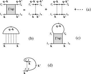
Figure 1: (a) Particle-particle ladder in the broken-symmetry phase. Conventions for four-momenta and Nambu indices are specified. Dots delimiting the potential (broken line) represent $\tau_{3}$ Pauli matrices. Only combinations with $\ell_{L}=\ell^{\prime}_{L}$ and $\ell_{R}=\ell^{\prime}_{R}$ occur owing to the regularization we have adopted for the potential. (b) Fermionic self-energy diagram associated with the expression (17) in the normal phase. (c) Fermionic self-energy diagram associated with the expressions (18) and (19) in the broken-symmetry phase. (d) BCS contribution (15) to the self-energy.

Note further that the above result for $v_{2}(0)$ can be cast in the bosonic form $v_{2}(0)=4\pi a_{B}/m_{B}$ with $a_{B}=2a_{F}$. The present theory thus describes the effective interaction between the composite bosons within the Born approximation, while improved theoriesPi-S-98 ; petrov for $a_{B}$ would give smaller values for the ratio $a_{B}/a_{F}$. These improvements will not be considered in the present paper.

Apart from the overall factor $-8\pi/(m^{2}a_{F})$ (and a sign difference in the off-diagonal component APS-02 ), the expressions (11) and (12) coincide with the normal and anomalous non-condensate bosonic Green’s functions within the Bogoliubov approximation FW , respectively. These expressions will be specifically exploited in Sec. IID, where the strong-coupling limit of the fermionic self-energy will be analyzed in detail.

In the normal phase, on the other hand, the BCS single-particle Green’s functions are replaced by the bare single-particle propagator ${\mathcal{G}}_{0}(p)=[i\omega_{n}-\xi({\mathbf{p}})]^{-1}$, while for arbitrary coupling the particle-particle ladder acquires the form:

$$\Gamma_{0}(q)=-\left\{\frac{m}{4\pi a_{F}}+\int\!\frac{d{\mathbf{p}}}{(2\pi)^{3}}\right.$$

$$\times\left[\frac{\tanh(\beta\xi({\mathbf{p}})/2)+\tanh(\beta\xi({\mathbf{p}-q})/2)}{2(\xi({\mathbf{p}})+\xi({\mathbf{p}-q})-i\Omega_{\nu})}\left.-\frac{m}{{\mathbf{p}}^{2}}\right]\right\}^{-1}\,.$$ (15)

In particular, in the strong-coupling limit the expression (15) reduces to

$$\Gamma_{0}(q)\,\simeq\,-\,\frac{8\pi}{m^{2}a_{F}}\,\frac{1}{i\Omega_{\nu}-{\mathbf{q}}^{2}/(4m)}\,,$$ (16)

which coincides (apart again from the overall factor $-8\pi/(m^{2}a_{F})$) with the free-boson Green’s function.

The above quantities constitute the essential ingredients of our theory for the fermionic self-energy and related quantities in the broken-symmetry phase. As shown in Ref. APS-02, , they also serve to establish a mapping between the fermionic and bosonic diagrammatic structures in the broken-symmetry phase, in a similar fashion to what was done in the normal phase Pi-S-98 .

II.1 Choice of the self-energy

In a recent study PPSC-02 of the single-particle spectral function in the normal phase based on the BCS-BEC crossover approach, the fermionic self-energy was taken of the form:

$$\Sigma_{0}(k)\,=\,-\,\frac{1}{\beta{\mathcal{V}}}\,\sum_{q}\,\Gamma_{0}(q)\,\,{\mathcal{G}}_{0}(q-k)$$ (17)

where ${\mathcal{V}}$ is the quantization volume and $k=({\bf k},\omega_{s})$ is again a four-vector notation with wave vector ${\bf k}$ and fermionic Matsubara frequency $\omega_{s}$ ($s$ integer). In this expression, $\Gamma_{0}(q)$ is given by Eq. (15) for arbitrary coupling and ${\mathcal{G}}_{0}(k)$ is the bare single-particle propagator. The self-energy diagram corresponding to the expression (17) is depicted in Fig. 1(b). The fermionic single-particle excitations are effectively coupled to a (bosonic) superconducting fluctuation mode, which reduces to a free composite boson in the strong-coupling limit. Physically, the choice (17) for the self-energy entails the presence of a pairing interaction above $T_{c}$, which can have significant influence on the single-particle (as well as other) properties.

In the present paper, we choose the self-energy in the broken-symmetry phase below $T_{c}$, with the aim of recovering the expression (17) when approaching $T_{c}$ from below and the Bogoliubov approximation for the composite bosons in the strong-coupling limit. To this end, we adopt the simplest approximations to describe fermionic as well as bosonic excitations in the broken-symmetry phase, which reduce to bare fermionic and free bosonic excitations in the normal phase, respectively. These are the BCS single-particle Green’s functions (10) (in the place of the bare single-particle propagator ${\mathcal{G}}_{0}$) and the particle-particle ladder (7) (in the place of its normal-phase counterpart $\Gamma_{0}$). By this token, the fermionic self-energy (17) is replaced by the following $2\times 2$ matrix:

$$\!\!\!\!\!\!\Sigma^{L}_{11}(k)=-\Sigma^{L}_{22}(-k)=-\frac{1}{\beta{\mathcal{V}}}\sum_{q}\Gamma_{11}(q){\mathcal{G}}_{11}(q-k)$$ (18)

$$\Sigma^{L}_{12}(k)=\Sigma^{L}_{21}(k)=-\frac{1}{\beta{\mathcal{V}}}\sum_{q}\Gamma_{12}(q){\mathcal{G}}_{12}(q-k)\phantom{111}$$ (19)

where the label $L$ refers to the particle-particle ladder. The corresponding self-energy diagram is depicted in Fig. 1(c).footnote-Nambu-arrows

The choice (18) and (19) for the self energy is made on physical grounds. A formal “ab initio” derivation of these expressions can also be done in terms of “conserving approximations” in the Baym-Kadanoff sense, that hold even in the broken-symmetry phase Baym-62 . In such a formal derivation, however, the single-particle Green’s functions entering Eqs.(18) and (19) (also through the particle-particle ladder (7)) would be required to be self-consistently determined with the same self-energy insertions. In our approach, we take instead the single-particle Green’s functions to be of the BCS form (10). The order parameter $\Delta$ and chemical potential $\mu$ are obtained, however, via two coupled equations (to be discussed in Sec. IIC) that include the self-energy insertions (18) and (19). In this way, we will recover the Bogoliubov form (11) and (12) for the particle-particle ladder not only at zero temperature but also at finite temperatures (and, in particular, close to the Bose-Einstein transition temperature).

The choice (18) and (19) for the self energy is not exhaustive. In the broken-symmetry phase there, in fact, exists an additional self-energy contribution that survives the regularization (1) of the interaction potential in the limit $k_{0}\rightarrow\infty$, even though it does not contain particle-particle rungsHaussmann-footnote . This additional self-energy diagram is the ordinary BCS contribution depicted in Fig. 1(d), with the associated expression

$$\Sigma^{BCS}_{12}(k)\,=\,\Sigma^{BCS}_{21}(k)\,=\,-\,\Delta\,\,,$$ (20)

while the corresponding (Hartree-Fock) diagonal elements vanish with the regularization we have adopted. Relating the expression (20) to the diagram of Fig. 1(d) rests on the validity of the BCS gap equation [Eq. (37) below], for arbitrary values of the chemical potential. For this, as well as for an additional reason (cf. Sec. IID), we shall consistently consider that equation to hold for the order parameter $\Delta$.

The choice (20) alone would be appropriate to describe the system in the weak-coupling (BCS) limit, where the superconducting fluctuation contributions (18) and (19) represent only small corrections. In the intermediate- and strong-coupling regions, on the other hand, both contributions (18)-(19) and (20) might become equally significant (depending on the temperature range below $T_{c}$). We thus consider both contributions simultaneously and write the fermionic self-energy in the matrix form:

$$\left(\begin{array}[]{cc}\Sigma_{11}(k)&\Sigma_{12}(k)\\ \Sigma_{21}(k)&\Sigma_{22}(k)\end{array}\right)\phantom{11111111111111111111111111}$$ (23)

$$=\left(\begin{array}[]{cc}\Sigma^{L}_{11}(k)&\Sigma^{L}_{12}(k)+\Sigma^{BCS}_{12}(k)\\ \Sigma^{L}_{21}(k)+\Sigma^{BCS}_{21}(k)&\Sigma^{L}_{22}(k)\end{array}\right)\,.$$ (26)

In the following, however, we shall neglect $\Sigma^{L}_{12}$ in comparison to $\Sigma^{BCS}_{12}$. It will, in fact, be proved in Sec. IID that, in strong coupling, $\Sigma^{L}_{12}$ is subleading with respect to both $\Sigma^{BCS}_{12}$ and $\Sigma^{L}_{11}$. Inclusion of $\Sigma^{L}_{12}$ is thus not required to properly recover the Bogoliubov description for the composite bosons in the strong-coupling limit.

To summarize, the fermionic single-particle Green’s functions are obtained in terms of the bare single-particle propagator ${\mathcal{G}}_{0}(k)$ and of the self-energy (18) and (20) via the Dyson’s equation in matrix form:

$$\left(\begin{array}[]{cc}G_{11}^{-1}(k)&G_{12}^{-1}(k)\\ G_{21}^{-1}(k)&G_{22}^{-1}(k)\end{array}\right)=\left(\begin{array}[]{cc}{\mathcal{G}}_{0}(k)^{-1}&0\\ 0&-{\mathcal{G}}_{0}(-k)^{-1}\end{array}\right)$$ (31)

$$-\left(\begin{array}[]{cc}\Sigma^{L}_{11}(k)&\Sigma^{BCS}_{12}(k)\\ \Sigma^{BCS}_{21}(k)&\Sigma^{L}_{22}(k)\end{array}\right)\,.$$ (34)

If only the BCS contribution (20) to the self-energy were retained, the fermionic single-particle Green’s functions $G_{ij}(k)$ ($i,j=1,2$) would reduce to the BCS form (10). Upon including, in addition, the fluctuation contribution (18) to the self-energy, modified single-particle Green’s functions result, which we are going to study as functions of coupling strength and temperature.

II.2 Comparison with the Popov approximation for dilute superfluid fermions

The choice of the self-energy (18) and (20) resembles the approximation for the self-energy introduced by PopovPopov-87 for superfluid fermions in the dilute limit $k_{F}|a_{F}|\ll 1$ (with $a_{F}<0$). There is, however, an important difference between the Popov fermionic approximation and our theory. We include in Eq. (18) the full $\Gamma_{11}$ obtained by the matrix inversion of Eq. (7); Popov instead neglects $\chi_{12}$ therein and approximate $\Gamma_{11}$ by $1/\chi_{11}$, thus removing the feedback of the Bogoliubov-Anderson mode on the diagonal fermionic self-energy $\Sigma_{11}$. Retaining this mode is essential when dealing with the BCS-BEC crossover, to describe the composite bosons in the strong-coupling limit by the Bogoliubov approximation, as discussed in Sec. IIA. Approaching the weak-coupling limit, on the other hand, the presence of the Bogoliubov-Anderson mode becomes progressively irrelevant and the self-energies coincide in the two theories. As a check on this point, we have verified that, in the weak-coupling limit and at zero temperature, $\Sigma_{11}$ obtained by our theory (using the numerical procedures discussed in Sec. III) reduces to $4\pi a_{F}n/(2m)$, which is the expression obtained also with the Popov approximationPopov-87 in the absence of the Bogoliubov-Anderson mode.

There is another difference between the Popov fermionic approximation and our theory as formulated in Sec. IIA, which concerns the off-diagonal fermionic self-energy $\Sigma_{12}$. Our expression (20) for $\Sigma_{12}$ was obtained from the diagram of Fig. 1(d), where the single particle line represents the off-diagonal BCS Green’s function of Eq. (10) with no insertion of the diagonal self-energy $\Sigma_{11}$. Within the Popov approximation, on the other hand, $\Sigma_{12}$ is defined formally by the same diagram of Fig. 1(d), but with the single-particle line being fully self-consistent (and thus including $\Sigma_{11}$). Since $\Sigma_{11}$ turns out to approach a constant value $\Sigma_{0}$ in the weak-coupling limit (as discussed above), inclusion of $\Sigma_{11}\simeq\Sigma_{0}$ can be simply made by a shift of the chemical potential (such that $\mu\to\mu-\Sigma_{0}$). This shift affects, however, the value of the gap function $\Delta$ in a non-negligible way even in the extreme weak-coupling limit. Neglecting this shift, in fact, results in a reduction by a factor $e^{1/3}$ of the BCS asymptotic expression $(8\epsilon_{F}/e^{2})\exp[\pi/(2k_{F}a_{F})]$ for $\Delta$ (where $\epsilon_{F}=k_{F}^{2}/(2m)$). Inclusion of the shift $\Sigma_{0}$ is thus important to recover the BCS value for $\Delta$ in the (extreme) weak-coupling limit.

The need to include the constant shift $\Sigma_{0}$ on the weak-coupling side of the crossover was also discussed in Ref. PPSC-02, while studying the spectral function $A({\bf k},\omega)$ in the normal phase with the inclusion of pairing fluctuations. In that context, inclusion of the shift $\Sigma_{0}$ proved necessary to have the pseudogap depression of $A({\bf k},\omega)$ centered about $\omega=0$. Inclusion of the shift $\Sigma_{0}$ in the broken-symmetry phase (at least when approaching the critical temperature from below) is thus also necessary to connect the spectral function $A({\bf k},\omega)$ with continuity in the weak-coupling side of the crossover.

Combining the above needs for $\Delta$ and $A({\bf k},\omega)$, we have introduced the constant shift $\Sigma_{0}$ for all temperatures below $T_{c}$, by replacing $\mu$ with $\mu-\Sigma_{0}$ in the BCS Green’s functions (10) entering the convolutions (8) and (9). The same replacement is made in the gap equation [Eq. (37) below]. In the Dyson’s equation (34), however, $\mu$ is left unchanged since the constant shift $\Sigma_{0}$ is already contained in $\Sigma_{11}(k)$ as soon as its $k$-dependence is irrelevant. Accordingly, we have included this constant shift in the calculation of both thermodynamic and dynamical quantities in the weak-coupling side for $(k_{F}a_{F})^{-1}\leq-0.5$, and neglected it for larger couplings when $\Sigma_{11}(k)$ can no longer be approximated by a constant.

Figure 2: Self-energy shift $\Sigma_{0}$ (in units of $\epsilon_{F}$) vs temperature $T$ (units of $T_{c}$) and coupling $(k_{F}a_{F})^{-1}$.

It turns out that the temperature dependence of $\Sigma_{0}$ is rather weak in the above coupling range. A plot of $\Sigma_{0}$ vs $T/T_{c}$ and $(k_{F}a_{F})^{-1}$ is shown in Fig. 2. Here, the critical temperature $T_{c}$ is obtained by applying the Thouless criterion from the normal phase as was done in Ref. PPSC-02, (this procedure to obtain $T_{c}$ will be used in the rest of the paper). In this plot, the constant shift $\Sigma_{0}$ is obtained as $\Sigma_{0}={\rm Re}\Sigma_{11}^{R}(|{\bf k}|=\sqrt{2m(\mu-\Sigma_{0})},\omega=0)$, in analogy to what was also done in Ref. PPSC-02, . Here, $\Sigma_{11}^{R}({\bf k},\omega)$ is the analytic continuation to the real frequency axis of the Matsubara self-energy $\Sigma_{11}({\bf k},\omega_{s})$ discussed in Sec. IIE.

II.3 Coupled equations for the order parameter and the chemical potential

Thermodynamic quantities, such as the order parameter $\Delta$ and the chemical potential $\mu$, are obtained directly in terms of the Matsubara single-particle Green’s functions, without the need of resorting to the analytic continuation to the real frequency axis.

Quite generally, the order parameter $\Delta$ is defined in terms of the “anomalous” Green’s function $G_{12}({\mathbf{k}},\omega_{s})$ via $\Delta=v_{0}\langle\psi_{\uparrow}({\mathbf{r}})\psi_{\downarrow}({\mathbf{r}})\rangle$ [cf. Eq. (88)], where the strength $v_{0}$ of the contact potential is kept to comply with a standard definition of BCS theory FW . One obtains:

$$\Delta\,=\,-\,v_{0}\,\int\!\frac{d{\mathbf{k}}}{(2\pi)^{3}}\,\frac{1}{\beta}\sum_{s}\,G_{12}({\mathbf{k}},\omega_{s})\,\,.$$ (35)

By the same token, the chemical potential $\mu$ can be obtained in terms of the “normal” Green’s function $G_{11}({\mathbf{k}},\omega_{s})$ via the particle density $n$:

$$n\,=\,2\,\int\!\frac{d{\mathbf{k}}}{(2\pi)^{3}}\,\frac{1}{\beta}\sum_{s}\,e^{i\omega_{s}\eta}\,G_{11}({\mathbf{k}},\omega_{s})$$ (36)

where $\eta=0^{+}$. The two equations (35) and (36) are coupled, since the Green’s functions depend on both $\Delta$ and $\mu$. The results of their numerical solution will be presented in the next section for various temperatures and couplings.

In the following treatment, we shall deal with the two equations (35) and (36) on a different footing. Specifically, we will enter in the density equation (36) the expression for the normal Green’s function obtained from Eq. (34), that includes both BCS and fluctuation contributions (see Eq. (57) below). We will use instead in the gap equation (35) the BCS anomalous function (10), that includes only the BCS self-energy (20). In this way, the gap equation (35) reduces to the form

$$\frac{m}{4\pi a_{F}}\,+\,\int\!\frac{d{\mathbf{k}}}{(2\pi)^{3}}\,\left[\frac{\tanh(\beta E({\mathbf{k}})/2)}{2E({\mathbf{k}})}\,-\,\frac{m}{{\mathbf{k}}^{2}}\right]\,=\,0$$ (37)

where the regularization of the contact potential in terms of the scattering length $a_{F}$ has been introduced. This equation has the same formal structure of the BCS gap equation, although the numerical values of the chemical potential entering Eq. (37) differ from those obtained by the BCS density equation. This procedure ensures that the bosonic propagators (7) in the broken-symmetry phase are gapless, as shown explicitly by the Bogoliubov-type expressions (11) and (12) in the strong-coupling limit. In general, in fact, there is no a priori guarantee that a given (conserving) approximation for fermions would result into a “gapless” approximation HM-65 for the composite bosons in the strong-coupling limit of the fermionic attraction.

Including fluctuation corrections to the BCS density equation as in Eq. (36), on the other hand, results in the emergence of important effects in the strong-coupling limit of the theory, as discussed next.

II.4 Analytic results in the strong-coupling limit

We proceed to show that the original fermionic theory, as defined by the Dyson’s equation (34), maps onto the Bogoliubov theory for the composite bosons which form as bound-fermion pairs in the strong-coupling limit. To this end, we shall exploit the conditions $\beta|\mu|\gg 1$ and $\Delta\ll|\mu|$ ($\mu<0$) (which define the strong-coupling limit) in the (Matsubara) expressions (18) and (19) for $\Sigma^{L}(p)$, thus also verifying that $\Sigma_{12}^{L}$ can be neglected.

These expressions are calculated by performing the wave-vector and frequency convolutions with the approximate expressions (11) and (12) for the particle-particle ladder and the expressions (10) for the BCS single-particle Green’s functions.

Upon neglecting contributions that are subleading under the above conditions, we obtain in this way for the diagonal part of the self-energy:

$$\Sigma_{11}^{L}({\mathbf{k}},\omega_{s}) \simeq \frac{8\pi}{m^{2}a_{F}}\int\!\frac{d{\mathbf{q}}}{(2\pi)^{3}}\left[\frac{u_{B}^{2}({\mathbf{q}})b(E_{B}({\mathbf{q}}))}{i\omega_{s}+E({\mathbf{q}}-{\bf k})-E_{B}({\mathbf{q}})}\right.$$ (38)

$$- \left.\frac{v_{B}^{2}({\mathbf{q}})b(-E_{B}({\mathbf{q}}))}{i\omega_{s}+E({\mathbf{q}}-{\bf k})+E_{B}({\mathbf{q}})}\right]\,.$$

In this expression, $E({\mathbf{k}})$ is the BCS dispersion of Eqs. (10), $E_{B}({\mathbf{q}})$ is the Bogoliubov dispersion relation (13), $b(x)=[\exp(\beta x)-1]^{-1}$ is the Bose distribution, and

$$v_{B}^{2}({\mathbf{q}})\,=\,u_{B}^{2}({\mathbf{q}})-1\,=\,\frac{\frac{{\mathbf{q}}^{2}}{2m_{B}}\,+\mu_{B}\,-\,E_{B}({\mathbf{q}})}{2E_{B}({\mathbf{q}})}$$ (39)

are the standard bosonic factors of the Bogoliubov transformation FW .

In the numerators of the expressions within brackets in Eq. (38), the Bose functions are peaked at about ${\mathbf{q}}=0$ and vary over a scale ${\mathbf{q}}^{2}/(2m_{B})\approx T\ll|\mu|$. Similarly, the factors $u_{B}^{2}({\mathbf{q}})$ and $v_{B}^{2}({\mathbf{q}})$ are also peaked at about ${\mathbf{q}}=0$ and vary over a scale ${\mathbf{q}}^{2}/(2m_{B})\approx\mu_{B}\ll|\mu|$. The denominators in the expression (38), on the other hand, vary over the much larger scale $|\mu|$. For these reasons, we can further approximate the expression (38) as follows:

$$\Sigma_{11}^{L}({\mathbf{k}},\omega_{s})\,\simeq\,\frac{8\pi}{m^{2}a_{F}}\,\,\frac{1}{i\omega_{s}+\xi({\mathbf{k}})}\,\,n^{\prime}_{B}(T)$$ (40)

where

$$n^{\prime}_{B}(T)=\int\!\frac{d{\mathbf{q}}}{(2\pi)^{3}}\left[u_{B}^{2}({\mathbf{q}})b(E_{B}({\mathbf{q}}))-v_{B}^{2}({\mathbf{q}})b(-E_{B}({\mathbf{q}}))\right]$$ (41)

identifies the bosonic noncondensate density according to Bogoliubov theory FW . Note that in the normal phase (when the condensate density $n_{0}(T)$ of Eq. (14) vanishes), the noncondensate density (41) becomes the full bosonic density $n_{B}=n/2$, and Eq. (40) reduces to the expression obtained in Ref. Pi-S-98, directly from the form (17) of the fermionic self-energy.

The off-diagonal self-energy $\Sigma_{12}^{L}(k)$ can be analyzed in a similar way. Since its magnitude is supposed to be the largest at zero temperature, we estimate it correspondingly for ${\mathbf{k}}=0$ and $\omega_{s}=0$ as follows:

$$\Sigma_{12}^{L}({\mathbf{k}}=0,\omega_{s}=0) \simeq \frac{8\pi}{m^{2}a_{F}}\frac{\mu_{B}\Delta}{2}\int\!\frac{d{\mathbf{k}^{\prime}}}{(2\pi)^{3}}\frac{1}{E({\mathbf{k}^{\prime}})E_{B}({\mathbf{k}^{\prime}})}$$ (42)

$$\times \frac{1}{(E({\mathbf{k}^{\prime}})\,+\,E_{B}({\mathbf{k}^{\prime}}))}\,\,.$$

At the leading order, we can neglect both $\Delta$ and $\mu_{B}$ in the integrand, where the energy scale $|\mu|$ dominates. We thus obtain $\Sigma_{12}^{L}(k=0)\approx\Delta(\Delta^{2}/(2|\mu|^{2}))$ in the strong-coupling limit (where the relation $\mu_{B}=\Delta^{2}/(4|\mu|)$ - see below - has been used). This represents a subleading contribution in the small dimensionless parameter $\Delta/|\mu|$ with respect to both the BCS contribution $\Sigma_{12}^{{\rm BCS}}(k)=-\Delta$ and the diagonal fluctuation contribution $\Sigma_{11}^{L}(k)$. It can accordingly be neglected.

Within the above approximations, the inverse (34) of the fermionic single-particle Green’s function reduces to:

$$\left(\begin{array}[]{cc}G_{11}^{-1}(k)&G_{12}^{-1}(k)\\ G_{21}^{-1}(k)&G_{22}^{-1}(k)\end{array}\right)\phantom{1111111111111111111111111}$$ (45)

$$\simeq\left(\begin{array}[]{cc}i\omega_{s}-\xi({\mathbf{k}})-\frac{\Delta_{0}^{2}}{i\omega_{s}+\xi({\mathbf{k}})}&\Delta\\ \Delta&i\omega_{s}+\xi({\mathbf{k}})-\frac{\Delta_{0}^{2}}{i\omega_{s}-\xi({\mathbf{k}})}\end{array}\right)$$ (48)

with the notation

$$\Delta_{0}^{2}\,\equiv\,\frac{8\pi}{m^{2}a_{F}}\,\,n^{\prime}_{B}(T)\;.$$ (49)

From Eq. (48) we get the desired expression for $G_{11}({\mathbf{k}},\omega_{s})$ in the strong-coupling limit:

$$G_{11}({\mathbf{k}},\omega_{s})\,\simeq\,\frac{1}{i\omega_{s}\,-\,\xi({\mathbf{k}})\,-\,\frac{\Delta^{2}\,+\,\Delta_{0}^{2}}{i\omega_{s}\,+\,\xi({\mathbf{k}})}}$$ (50)

where we have discarded a term of order $\Delta_{0}^{2}/|\mu|$ with respect to $|\mu|$. Note that Eq. (50) has the same formal structure of the corresponding BCS expression (10), with the replacement $E({\mathbf{k}})\rightarrow\tilde{E}({\mathbf{k}})=\sqrt{\xi({\mathbf{k}})^{2}+(\Delta^{2}+\Delta_{0}^{2})}$. We rewrite it accordingly as:

$$G_{11}({\mathbf{k}},\omega_{s})\,\simeq\,\frac{\tilde{u}^{2}({\mathbf{k}})}{i\omega_{s}\,-\,\tilde{E}({\mathbf{k}})}\,+\,\frac{\tilde{v}^{2}({\mathbf{k}})}{i\omega_{s}\,+\,\tilde{E}({\mathbf{k}})}$$ (51)

with the modified BCS coherence factors $\tilde{v}^{2}({\mathbf{k}})=1-\tilde{u}^{2}({\mathbf{k}})=(1-\xi({\mathbf{k}})/\tilde{E}({\mathbf{k}}))/2$.

Before making use of the asymptotic expression (51) in the density equation (36), it is convenient to manipulate suitably the gap equation (37) in the strong-coupling limit. Expanding $1/E({\mathbf{k}})$ therein as $[1-\Delta^{2}/(2\xi({\mathbf{k}})]/\xi({\mathbf{k}})$ and evaluating the resulting elementary integrals, one obtains:

$$\frac{\Delta^{2}}{4|\mu|}\,\simeq\,2\,\left(\sqrt{2\,|\mu|\,\epsilon_{0}}\,-\,2\,|\mu|\right)\,.$$ (52)

Setting further $2\mu=-\epsilon_{0}+\mu_{B}$, one gets the relation $\Delta^{2}/(4|\mu|)=\mu_{B}$ quoted already after Eqs. (13) and (42).

Let’s now consider the density equation (36). With the BCS-like form (51) one obtains immediately:

$$n\,\simeq\,2\,\int\!\frac{d{\mathbf{k}}}{(2\pi)^{3}}\,\tilde{v}^{2}({\mathbf{k}})$$ (53)

that holds for $T\ll\epsilon_{0}$, at temperatures well below the dissociation threshold of the composite bosons. Similarly to what was done to get the gap equation (52), in Eq. (53) one expands $1/\tilde{E}({\mathbf{k}})$ as $[1-(\Delta^{2}+\Delta_{0}^{2})/(2\xi({\mathbf{k}})]/\xi({\mathbf{k}})$ and evaluates the resulting elementary integrals, to obtain:

$$n\,\simeq\,\frac{m^{2}\,a_{F}}{4\pi}\,\,\left(\Delta^{2}\,+\,\Delta_{0}^{2}\right)\,\,.$$ (54)

Recalling the definition (49) for $\Delta_{0}^{2}$, as well as the expressions (52) and (14) for the order parameter, which we rewrite in the form

$$\Delta^{2}\,=\,\frac{8\pi}{m^{2}a_{F}}\,\,n_{0}(T)$$ (55)

in analogy to Eq. (49), the result (54) becomes eventually:

$$n\,=\,2\left(n^{\prime}_{B}(T)\,+\,n_{0}(T)\right)$$ (56)

that holds asymptotically for $T\ll\epsilon_{0}$.

These results imply that, in the strong-coupling limit, the original fermionic theory recovers the Bogoliubov theory for the composite bosons, not only at zero temperature but also at any temperature in the broken-symmetry phase. Accordingly, the noncondensate density $n^{\prime}_{B}(T)$ is given by the expression (41), the bosonic factors $v_{B}^{2}({\mathbf{q}})$ and $u_{B}^{2}({\mathbf{q}})$ are given by Eq. (39), and the dispersion relation $E_{B}({\mathbf{q}})$ is given by Eq. (13). In the strong-coupling limit, the present fermionic theory thus inherits all virtues and shortcomings of the Bogoliubov theory for a weakly-interacting Bose gas Bassani-GCS-01 . The present fermionic theory at arbitrary coupling then provides an interpolation procedure between the Bogoliubov theory for the composite bosons and the weak-coupling BCS theory plus pairing fluctuations. Both these analytic limits will constitute important checks on the numerical calculations reported in Sec. III. Note that inclusion of the off-diagonal fluctuation contribution $\Sigma_{12}^{L}(k)$ to the self-energy is not required to recover the Bogoliubov theory in strong coupling. For this reason, we will not consider $\Sigma_{12}^{L}(k)$ altogether in the numerical calculations presented in Sec. III, as anticipated in Eq. (34).

The above analytic results enable us to infer the main features of the temperature dependence of the order parameter in the strong-coupling limit. In particular, the low-temperature behavior $n_{0}(T)=n_{0}(0)-m_{B}(k_{B}T)^{2}/(12c)$( where $c=\sqrt{n_{0}v_{2}(0)/m_{B}}$ is the sound velocity) within the Bogoliubov approximation, implies that $\Delta(T)$ decreases from $\Delta(0)$ with a $T^{2}$ behavior, in the place of the exponential behavior obtained within the BCS theory (with an $s$-wave order parameter) FW . In addition, in the present theory the order parameter vanishes over the scale of the Bose-Einstein transition temperature $T_{BE}$, while in the BCS theory it would vanish over the scale of the bound-state energy $\epsilon_{0}$ of the composite bosons.

Note finally that the fermionic quasi-particle dispersion $\tilde{E}({\mathbf{k}})$, entering the expression (51) of the diagonal Green’s function in the strong-coupling limit, contains the sum $\Delta^{2}+\Delta_{0}^{2}$ instead of the single term $\Delta^{2}$ of the BCS dispersion $E({\mathbf{k}})$.

II.5 Spectral function and sum rules

We pass now to identify the form of the spectral function $A({\mathbf{k}},\omega)$ associated with the approximate choice of the Matsubara self-energy of Eq. (34). To this end, we need to perform the analytic continuation in the complex frequency plane, thus determining the retarded fermionic single-particle Green’s functions from their Matsubara counterparts. The approach developed in this subsection holds specifically for the approximate choice for the self-energy of Eq. (34). It thus differs from the general analysis presented in the Appendix which holds for the exact Green’s functions, irrespective of any specific approximation.

In general, the process of analytic continuation to the real frequency axis from the numerical Matsubara Green’s functions proves altogether nontrivial, as it requires in practice recourse to approximate numerical methods such as, e.g., the method of Padé approximants Serene-1977 . We then prefer to rely on a procedure whereby the analytic continuation to the real frequency axis is achieved by avoiding numerical extrapolations from the Matsubara Green’s functions.

The fermionic normal and anomalous Matsubara single-particle Green’s functions are obtained at any given coupling from matrix inversion of Eq. (34):

$$G_{11}({\mathbf{k}},\omega_{s})=\left[\phantom{\frac{1}{1}}\!\!\!i\omega_{s}-\xi({\mathbf{k}})-\Sigma_{11}({\mathbf{k}},\omega_{s})\right.$$

$$\phantom{111111111}-\left.\frac{\Delta^{2}}{i\omega_{s}+\xi({\mathbf{k}})-\Sigma_{22}({\mathbf{k}},\omega_{s})}\right]^{-1}$$ (57)

$$G_{12}({\mathbf{k}},\omega_{s})=\Delta[\,(i\omega_{s}-\xi({\mathbf{k}})-\Sigma_{11}({\mathbf{k}},\omega_{s}))$$

$$\phantom{1111}\times(i\omega_{s}+\xi({\mathbf{k}})-\Sigma_{22}({\mathbf{k}},\omega_{s}))-\Delta^{2}]^{-1}\;.$$ (58)

Consider first the normal Green’s function (57), which we rewrite in the compact form

$$G_{11}({\mathbf{k}},\omega_{s})\,=\,\frac{1}{i\omega_{s}-\xi({\mathbf{k}})-\sigma_{11}({\mathbf{k}},\omega_{s})}$$ (59)

with the short-hand notation

$$\sigma_{11}({\mathbf{k}},\omega_{s})\,\equiv\,\Sigma_{11}({\mathbf{k}},\omega_{s})\,+\,\frac{\Delta^{2}}{i\omega_{s}\,\,+\,\,\xi({\mathbf{k}})-\,\,\Sigma_{22}({\mathbf{k}},\omega_{s})}\,\,.$$ (60)

To perform the analytic continuation of this expression, we look for a function $\sigma_{11}({\mathbf{k}},z)$ of the complex frequency $z$ which satisfies the following requirements at any given ${\mathbf{k}}$:
(i) It is analytic off the real axis;
(ii) It reduces to $\sigma_{11}({\mathbf{k}},\omega_{s})$ given by Eq. (60) when $z$ takes the discrete values $i\omega_{s}$ on the imaginary axis;
(iii) Its imaginary part is negative (positive) for $\mathrm{Im}\,z>0$ ($\mathrm{Im}\,z<0$) ;
(iv) It vanishes when $|z|\to\infty$ along any straight line parallel to the real axis with $\mathrm{Im}\,z\neq 0$.

Once the function $\sigma_{11}({\mathbf{k}},z)$ is obtained, the expression

$$G^{R}({\mathbf{k}},\omega)\,=\,\frac{1}{\omega\,+\,i\eta\,-\,\xi({\mathbf{k}})\,-\,\sigma_{11}({\mathbf{k}},\omega+i\eta)}$$ (61)

($\eta$ being a positive infinitesimal) represents the retarded ($R$) single-particle Green’s function (for real $\omega$) associated with the Matsubara Green’s function (59), since it satisfies the requirements of the Baym-Mermin theorem Baym-Mermin-61 for the analytic continuation from the Matsubara Green’s function.

The first step of the above program is to find the analytic continuation of $\Sigma_{11}({\mathbf{k}},\omega_{s})$ (and $\Sigma_{22}({\mathbf{k}},\omega_{s})$) off the real axis in the complex $z$-plane. To this end, it is convenient to express $\Sigma_{11}({\mathbf{k}},\omega_{s})$ via the spectral form:

$$\Sigma_{11}({\mathbf{k}},\omega_{s})=\int_{-\infty}^{+\infty}\frac{d\omega^{\prime}}{\pi}\frac{h({\mathbf{k}},\omega^{\prime})}{i\omega_{s}-\omega^{\prime}}\;\,.$$ (62)

With the replacement $i\omega_{s}\to z$, the spectral representation (62) defines an analytic function $\Sigma_{11}({\mathbf{k}},z)$ off the real axis. In the case of interest with $\Sigma_{11}({\mathbf{k}},\omega_{s})$ given by Eq. (18), the function $h({\mathbf{k}},\omega)$ of Eq. (62) reads:

$$h({\bf k},\omega) = -\int\frac{d{\bf q}}{(2\pi)^{3}}\left\{u^{2}_{{\bf q}-{\bf k}}{\rm Im}\,\Gamma_{11}^{R}({\bf q},\omega+E({\bf q}-{\bf k}))\right.$$ (63)

$$\times \left[f(E({\bf q}-{\bf k}))+b(\omega+E({\bf q}-{\bf k}))\right]$$

$$+ v^{2}_{{\bf q}-{\bf k}}{\rm Im}\,\Gamma_{11}^{R}({\bf q},\omega-E({\bf q}-{\bf k}))$$

$$\times \left.\left[f(-E({\bf q}-{\bf k}))+b(\omega-E({\bf q}-{\bf k}))\right]\right\}$$

where $f(x)=[\exp(\beta x)+1]^{-1}$ is the Fermi distribution while $u^{2}_{{\bf k}}$ and $v^{2}_{{\bf k}}$ are the BCS coherence factors. To obtain the expression (63), a spectral representation has been also introduced for $\Gamma_{11}$ entering Eq. (18), by writing:

$$\Gamma_{11}({\mathbf{q}},\Omega_{\nu})\,=-\frac{1}{\pi}\int_{-\infty}^{+\infty}\!d\omega^{\prime}\,\frac{{\rm Im}\,\Gamma_{11}^{R}({\mathbf{q}},\omega^{\prime})}{i\Omega_{\nu}-\omega^{\prime}}\;.$$ (64)

Here, the spectral function $\Gamma_{11}^{R}({\mathbf{q}},\omega)$ is defined by $\Gamma_{11}({\mathbf{q}},i\Omega_{\nu}\rightarrow\omega+i\eta)$, which is obtained from the definitions (7)-(9) with the replacement $i\Omega_{\nu}\rightarrow\omega+i\eta$ after the sum over the internal frequency $\omega_{n}$ has been performed therein. Even in the absence of an explicit Lehmann representation for $\Gamma_{11}$, in fact, it can be shown that the spectral representation (64) holds provided the function $\Gamma_{11}({\mathbf{q}},i\Omega_{\nu}\to z)$ of the complex variable $z$ is analytic off the real axis. The crucial point is to verify that the denominator in Eq. (7) with the replacement $i\Omega_{\nu}\to z$ never vanishes off the real axis. This property can be explicitly verified in the strong-coupling limit, as discussed below. For arbitrary coupling, we have checked it with the help of numerical calculations. For the validity of the expression $(\ref{spectral-representation})$, it is also required that $\Gamma_{11}({\mathbf{q}},z)$ vanishes for $|z|\to\infty$. This property can be proved directly from Eqs. (7)-(9), according to which $\Gamma_{11}({\mathbf{q}},z)$ has the asymptotic expression

$$\Gamma_{11}({\bf q},z)\simeq\frac{-1}{\frac{m}{4\pi a_{F}}-\frac{m^{3/2}}{4\pi}\sqrt{-z+{q^{2}\over 4m}-2\mu}}$$ (65)

and thus vanishes for $|z|\to\infty$. Once $\Sigma_{11}({\mathbf{k}},z)$ has been explicitly constructed according to the above prescriptions, $\Sigma_{22}({\mathbf{k}},z)$ is obtained as $-\Sigma_{11}({\mathbf{k}},-z)$ in accordance with Eq. (18).

From the spectral representation (62) for $\Sigma_{11}({\mathbf{k}},z)$, it can be further shown that $\Sigma_{11}({\mathbf{k}},z)$ vanishes when $|z|\to\infty$ along any straight line parallel to the real axis with ${\rm Im}\,\,z\neq 0$. It can also be shown that ${\rm Im}\,\Sigma_{11}({\mathbf{k}},z)<0$ (${\rm Im}\,\Sigma_{11}({\mathbf{k}},z)>0$) when ${\rm Im}\,z>0$ (${\rm Im}\,z<0$). This property follows from the spectral representation of $\Sigma_{11}({\mathbf{k}},z)$, provided $h({\bf k},\omega)\geq 0$ in Eq. (62). For arbitrary coupling, we have verified that $h({\bf k},\omega)\geq 0$ with the help of numerical calculations. In the strong-coupling limit, this condition can be explicitly proved, as discussed below.

From these properties of $\Sigma_{11}({\mathbf{k}},z)$ (and $\Sigma_{22}({\mathbf{k}},z)$) it can then be verified that the function

$$\sigma_{11}({\mathbf{k}},z) = \Sigma_{11}({\mathbf{k}},z)$$ (66)

$$+ \frac{\Delta^{2}}{z\,+\,\xi({\mathbf{k}})+\,\Sigma_{11}({\mathbf{k}},-z)},$$

satisfies the requirements (i)-(iv) stated after Eq. (60). With the replacement $z\to\omega+i\eta$, Eq. (61) follows eventually on the real frequency axis for the retarded Green’s function $G^{R}({\bf k},\omega)$.

For later convenience, we introduce the following notation on the real frequency axis :

$$\Sigma_{11}^{R}({\mathbf{k}},\omega)\equiv\Sigma_{11}({\mathbf{k}},\omega+i\eta)$$ (67)

such that $\Sigma_{11}({\mathbf{k}},-\omega-i\eta)=\Sigma_{11}^{R}({\mathbf{k}},-\omega)^{*}$ and

$$\sigma_{11}^{R}({\mathbf{k}},\omega)\equiv\sigma_{11}({\mathbf{k}},\omega+i\eta)\phantom{1111111111111111111}$$

$$=\Sigma_{11}^{R}({\mathbf{k}},\omega)\,+\,\frac{\Delta^{2}}{\omega+i\eta\,+\,\xi({\mathbf{k}})+\,\Sigma_{11}^{R}(-{\mathbf{k}},-\omega)^{*}}\;.$$ (68)

From Eq. (62) it is also clear that ${\rm Im}\,\Sigma_{11}^{R}({\mathbf{k}},\omega)=-h({\mathbf{k}},\omega)$, and that ${\rm Re}\Sigma_{11}^{R}({\mathbf{k}},\omega)$ and ${\rm Im}\,\Sigma_{11}^{R}({\mathbf{k}},\omega)$ are related by a Kramers-Kronig transform.

As anticipated, the properties of the function $\Sigma_{11}({\bf k},z)$, required above to obtain the retarded Green’s function (61) on the real axis, can be explicitly verified in the strong-coupling limit without recourse to numerical calculations. In this case, the approximate expression (11) can be used for $\Gamma_{11}$. This can be cast in the form (64), with

$${\rm Im}\,\,\Gamma_{11}^{R}({\bf q},\omega) = -\frac{8\pi^{2}}{m^{2}a_{F}}[v_{B}^{2}({\bf q})\delta(\omega+E_{B}({\mathbf{q}}))$$ (69)

$$\phantom{11111}-u_{B}^{2}({\bf q})\delta(\omega-E_{B}({\mathbf{q}}))]\;.$$

Entering the expression (69) into Eq. (63) and the resulting expression into Eq. (62), one obtains for $\Sigma_{11}({\bf k},\omega_{s})$ the sum of four terms:

$$\Sigma_{11}({\bf k},\omega_{s})=-\frac{8\pi}{m^{2}a_{F}}$$ (70)

$$\times\int\!\frac{d{\mathbf{q}}}{(2\pi)^{3}}\left\{u_{B}^{2}({\mathbf{q}})u^{2}_{{\bf q}-{\bf k}}\frac{b(E_{B}({\mathbf{q}}))+f(E({\bf q}-{\bf k}))}{E_{B}({\bf q})-E({\bf q}-{\bf k})-i\omega_{s}}\right.$$

$$+ \left.u_{B}^{2}({\mathbf{q}})v^{2}_{{\bf q}-{\bf k}}\frac{b(E_{B}({\mathbf{q}}))+f(-E({\bf q}-{\bf k}))}{E_{B}({\bf q})+E({\bf q}-{\bf k})-i\omega_{s}}\right.$$

$$+ \left.v_{B}^{2}({\mathbf{q}})u^{2}_{{\bf q}-{\bf k}}\frac{b(-E_{B}({\mathbf{q}}))+f(E({\bf q}-{\bf k}))}{E_{B}({\bf q})+E({\bf q}-{\bf k})+i\omega_{s}}\right.$$

$$+ \left.v_{B}^{2}({\mathbf{q}})v^{2}_{{\bf q}-{\bf k}}\frac{b(-E_{B}({\mathbf{q}}))+f(-E({\bf q}-{\bf k}))}{E_{B}({\bf q})-E({\bf q}-{\bf k})+i\omega_{s})}\right\}\;.$$

Since in strong coupling $f(E({\bf k}))\to 0$, $u^{2}_{{\bf k}}\to 1$, and $v^{2}_{{\bf k}}\to 0$, the second and fourth term within braces on the right-hand side of the Matsubara expression (70) may be dropped. The simplified expression (38) then results from Eq. (70). In the strong-coupling limit, one would then be tempted to perform the analytic continuation $i\omega_{s}\to z$ directly from the expression (38). Care must, however, be exerted on this point since the processes of taking the strong-coupling limit and performing the analytic continuation may not commute. By performing the analytic continuation $i\omega_{s}\to z$ directly in Eq. (70) one, in fact, obtains two additional terms with respect to the analytic continuation of Eq. (38). These two additional terms cannot be dropped a priori by the presence of the small factor $v^{2}_{{\bf q}-{\bf k}}$ in the strong-coupling limit, because for real $z$ the corresponding energy denominators may vanish. Retaining properly these two additional terms indeed affects in a qualitative way the spectral function $A({\bf k},\omega)$ in the strong-coupling limit, as discussed in Sec. III.

With the expression obtained by the analytic continuation $i\omega_{s}\to z$ of Eq. (70), one can prove explicitly that $\Sigma_{11}({\bf k},z)$ is analytic off the real axis and vanishes like $z^{-1}$ along any straight line parallel to the real axis with ${\rm Im}\,\,z\neq 0$, and that ${\rm sgn}[{\rm Im}\,\Sigma_{11}({\bf k},z)]=-{\rm sgn}[{\rm Im}\,\,z]$. In this way, the properties of the function $\Sigma_{11}({\bf k},z)$, required to obtain the retarded Green’s function (61) on the real axis, are explicitly verified in the strong-coupling limit.

Once the retarded Green’s function has been obtained in the form (61) according to the above prescriptions, its imaginary part defines the spectral function

$$A({\mathbf{k}},\omega)\equiv-(1/\pi)\mathrm{Im}\,G^{R}({\mathbf{k}},\omega)$$ (71)

which will be calculated numerically in Sec. III for a wide range of temperatures and couplings. In the Appendix, it is shown at a formal level that $A({\mathbf{k}},\omega)$ satisfies the sum rule (82). This sum rule will be considered an important test for the numerical calculations of Sec. III. To this end, it is necessary to prove that the sum rule (82) holds even for our approximate theory based on the Dyson’s equation (34).

To prove the sum rule (82) for the approximate theory, it is sufficient that the approximate $G_{11}({\bf k},z)$ (from which the retarded Green’s function (61) results when $z=\omega+i\eta$) behaves like $z^{-1}$ for large $|z|$. This property is verified by our theory, as shown above. As a consequence:

$$\int_{-\infty}^{+\infty}\!d\omega\,A({\mathbf{k}},\omega)=-\frac{1}{\pi}\,\mathrm{Im}\left[\int_{-\infty}^{\infty}\!d\omega\,G^{R}({\mathbf{k}},\omega)\right]$$

$$=-\frac{1}{\pi}\,\mathrm{Im}\left[-\oint_{C}\!d\omega\,G_{11}({\mathbf{k}},z)\right]=1\;$$ (72)

where the contour $C$ is a half-circle in the upper-half complex plane with center in the origin, large radius (such that the approximation $G_{11}({\mathbf{k}},z)\sim z^{-1}$ is valid), and counterclockwise direction.

Finally, the analytic continuation of the anomalous Matsubara single-particle Green’s function (58) can be obtained by following the same procedure adopted for the normal Green’s function (57). One writes for the retarded anomalous Green’s function

$$F^{R}({\bf k},\omega)=\Delta[(\omega+i\eta-\xi({\mathbf{k}})-\Sigma_{11}^{R}({\mathbf{k}},\omega))$$

$$\times(\omega+i\eta+\xi({\mathbf{k}})+\Sigma_{11}^{R}(-{\mathbf{k}},-\omega)^{*})-\Delta^{2}]^{-1}\;.$$ (73)

in the place of Eqs. (61) and (68). In this case, the analytic properties of $\Sigma_{ii}({\mathbf{k}},z)$ ($i=1,2$) discussed above imply that $G_{12}({\mathbf{k}},z)\sim-\Delta/z^{2}$ asymptotically for large $|z|$. As a consequence, the imaginary part of $F^{R}({\bf k},\omega)$

$$B({\mathbf{k}},\omega)\equiv-(1/\pi){\mathrm{I}m}\,F^{R}({\mathbf{k}},\omega)$$ (74)

satisfies the two following sum rules:

$$\int_{-\infty}^{+\infty}\!d\omega\,B({\mathbf{k}},\omega)\,=\,0$$ (75)

and

$$\int_{-\infty}^{+\infty}\!d\omega\,B({\mathbf{k}},\omega)\,\omega\,=\,-\,\Delta\,\,.$$ (76)

These sum rules can be verified by introducing the contour $C$ as in Eq. (72). Note again that these sum rules (which are proved on general grounds in the Appendix for the exact anomalous retarded single-particle Green’s function) follow here from our approximate form of $F^{R}({\mathbf{k}},\omega)$ only on the basis of the properties of analyticity. Verifying numerically the sum rules (72), (75), and (76) at any coupling and temperature will, in practice, constitute an important check on the validity of the above procedure for the analytic continuation.

An additional numerical check on the validity of the whole procedure at intermediate-to-weak coupling will be provided by the merging of the results, obtained by calculating the spectral function $A({\mathbf{k}},\omega)$ when approaching $T_{c}$ from below, with the results previously obtained in the normal phasePPSC-02 when approaching $T_{c}$ from above.

III Numerical results and discussion

In this section we present the numerical results based on the formal theory developed in Sec. II. Specifically, in Sec. IIIA we present the results obtained by solving the coupled equations (36) and (37) for the order parameter and chemical potential. Section IIIB deals instead with the numerical calculation of the spectral function (71) in the broken-symmetry phase, over the whole coupling range from weak to strong.

III.1 Order parameter and chemical potential

Before presenting the numerical results for $\Delta$ and $\mu$, it is worth outlining briefly the numerical procedure we have adopted.

At given temperature and coupling, the coupled equations (36) and (37) for the unknowns $\Delta$ and $\mu$ are solved via the Newton’s method. This requires knowledge of the self-energy $\Sigma_{11}({\bf k},\omega_{s})$ of Eq. (18), with $\Gamma_{11}(q)$ obtained from Eqs. (7)-(9). [As anticipated, in the numerical calculations we neglect $\Sigma_{12}^{L}$ in comparison to $\Sigma_{12}^{{\rm BCS}}$, since inclusion of $\Sigma_{12}^{L}$ is not required to recover the Bogoliubov results in the strong-coupling limit, as shown in Sec. IID.]

To this end, the frequency sums in Eqs. (8) and (9) are evaluated analytically, while the remaining wave-vector integral is calculated numerically by the Gauss-Legendre method. In particular, the radial wave-vector integral extending up to infinity is partitioned into an inner and an outer region, with the transformation $|{\bf p}|\to 1/|{\bf p}|$ exploited in the outer region.

The bosonic frequency sum in Eq. (18) requires special care, owing to its slow convergence and the lack of an intrinsic energy cutoff within our continuum model. We have accordingly partitioned this frequency sum into three regions, separated by the frequency scales $\Omega_{c_{1}}$ and $\Omega_{c_{2}}$ (with $0<\Omega_{c_{1}}<\Omega_{c_{2}})$. For $|\Omega_{\nu}|<\Omega_{c_{1}}$, the frequency sum is calculated explicitly. For $\Omega_{c_{1}}<|\Omega_{\nu}|<\Omega_{c_{2}}$, the frequency sum is approximated with great accuracy by the corresponding numerical integral, owing to the slow dependence of $\Gamma_{11}$ on $\Omega_{\nu}$. Finally, the tail of the frequency sum for $\Omega_{c_{2}}<|\Omega_{\nu}|$ (where the asymptotic expression (65) yields $\Gamma_{11}\propto(i\Omega_{\nu})^{-1/2}$) is evaluated analytically. Typically, $\Omega_{c_{1}}$ is taken of the order of the largest among the energy scales $|\omega_{s}|,\Delta,|\mu|,{\bf q}^{2}/(2m)$, and ${\bf k}^{2}/(2m)$; $\Omega_{c_{2}}$ is then taken at least ten times $\Omega_{c_{1}}$. It turns out that it is most convenient to apply this procedure to the frequency sum in Eq. (18) after the integration over the two angular variables of the wave vector ${\bf q}$ has been performed analytically; the remaining radial wave-vector integration is then performed numerically, with a cutoff much larger than the wave-vector scales $|{\bf k}|,\sqrt{2m\Delta}$, and $\sqrt{|\mu|}$.

Figure 3: Order parameter $\Delta$ (in units of $\epsilon_{F}$) vs temperature (in units of $T_{c}$) for different values of the coupling $(k_{F}a_{F})^{-1}$. Results obtained by the inclusion of fluctuations (full lines) are compared with mean-field results (dashed lines).

Finally, the frequency sum in the particle number equation (36) is evaluated by adding and subtracting the BCS Green’s function ${\cal G}_{11}$ on the right-hand side of that equation, in order to speed up the numerical convergence. Matsubara frequencies are here summed numerically up to a cutoff frequency, beyond which the sum is approximated by the corresponding numerical integral. The radial part of the wave-vector integral in Eq. (36) is also calculated numerically up to a cutoff scale beyond which a power-law decay sets in, so that the contribution from the tail can be calculated analytically.

With the above numerical prescriptions, we have obtained the behavior of $\Delta$ and $\mu$ vs temperature and coupling reported in Figs. 3-6.

Specifically, Fig. 3 shows the order parameter $\Delta$ vs temperature for different couplings [$(k_{F}a_{F})^{-1}=-0.5,0.5,1.2$, from top to bottom], in the window $-1\lesssim(k_{F}a_{F})^{-1}\lesssim+1$ where the crossover from weak to strong coupling is exhausted. Comparison is made with the corresponding curves obtained within mean field (dashed lines), when the BCS Green’s function ${\mathcal{G}}_{11}$ enters Eq. (36) in the place of the dressed $G_{11}$. In these plots, the temperature is normalized with respect to the critical temperature $T_{c}$ for the given coupling. This comparison shows that fluctuation corrections on top of mean field get progressively important at given coupling as the temperature is raised toward $T_{c}$. Close to $T_{c}$, fluctuation corrections become even more important upon approaching the strong-coupling limit. Near zero temperature, on the other hand, fluctuation corrections become negligible when approaching strong coupling. This confirms the expectation that, near zero temperature, the BCS mean field should be rather accurate both in the weak- and strong-coupling limits Leggett-80 .

Note from Fig. 3 that $\Delta$ jumps discontinuously close to the critical temperature when fluctuations are included on top of mean field. This jump becomes more evident as the coupling is increased. It reflects an analogous behavior of the condensate density near the critical temperature as obtained by the Bogoliubov theory for point-like bosons Luban . In the present theory this jump is carried over to the composite bosons, even at fermionic couplings [as in the middle panel of Fig. 3 ] when the composite bosons are not yet fully developed. When the fermionic coupling increases beyond the values reported in Fig. 3, however, the residual interaction between the composite bosons decreases further and the jump becomes progressively smaller. More refined theories for point-like bosons (see, e.g., Ref. griffin, ) remove the jump of the bosonic condensate density, which thus should be considered as an artifact of the Bogoliubov approximation. Apart from this jump, note that when the temperature is decreased below $T_{c}$ the order parameter $\Delta$ grows more rapidly with the inclusion of fluctuations than within mean field.

Figure 4: Chemical potential $\mu$ (in units of $\epsilon_{F}$) vs temperature (in units of $T_{c}$), for the same values of the coupling $(k_{F}a_{F})^{-1}$ as in Fig. 3.

Figure 4 shows the chemical potential $\mu$ vs temperature for the same coupling values of Fig. 3. Note that in weak coupling the chemical potential decreases slightly upon moving deep in the superconducting phase from $T_{c}$ to $T=0$, in agreement with the BCS behavior. In strong coupling the opposite occurs, reflecting the behavior of the bosonic chemical potential $\mu_{B}=2\mu+\epsilon_{0}$ within the Bogoliubov theory. It should be, however, mentioned that with improved bosonic approximations griffin , the bosonic chemical potential would rather decrease upon entering the condensed phase.

Figure 5: Order parameter $\Delta$ at $T=0$ (in units of $\epsilon_{F}$) vs the coupling $(k_{F}a_{F})^{-1}$ . Results obtained by the inclusion of fluctuations (full line) are compared with mean-field results (dashed line).

Figure 5 shows the order parameter $\Delta$ at zero temperature (full line) and the corresponding mean-field value (dashed line) vs the coupling $(k_{F}a_{F})^{-1}$. While $\Delta$ increases monotonically in absolute value from weak to strong coupling (as expected on physical grounds), the relative importance of the fluctuation corrections to the order parameter at zero temperature (over and above mean field) reaches a maximum in the intermediate-coupling region, never exceeding about 30%. This results confirms again that the BCS mean field is a reasonable approximation to the ground state for all couplings.

Figure 6 shows the chemical potential $\mu$ at zero temperature vs the coupling parameter $(k_{F}a_{F})^{-1}$. The results obtained by the inclusion of fluctuations (full lines) are compared with mean field (dashed lines). Even for this thermodynamic quantity the fluctuation corrections to the mean-field results appear to be not too important at zero temperature.

Note, finally, that the values for $\Delta$ and $\mu$ obtained from our theory at $T=0$ with the coupling value $(k_{F}a_{F})^{-1}=0$ are in remarkable agreement with a recent Quantum Monte Carlo calculation carlson performed for the same coupling. Our calculation yields, in fact, $\Delta/\epsilon_{F}=0.53$ and $\mu/\epsilon_{F}=0.445$, to be compared with the values $\Delta/\epsilon_{F}=0.54$ and $\mu/\epsilon_{F}=0.44\pm 0.01$ of Ref. carlson, . [In contrast, BCS mean field yields $\Delta/\epsilon_{F}=0.69$ and $\mu/\epsilon_{F}=0.59$.]

Figure 6: Chemical potential $\mu$ at $T=0$ (in units of $\epsilon_{F}$ for $\mu>0$ and of $\epsilon_{0}/2$ for $\mu<0$) vs the coupling $(k_{F}a_{F})^{-1}$. Results obtained by the inclusion of fluctuations (full line) are compared with mean-field results (dashed line).

In summary, the above results have shown that, for thermodynamic quantities like $\Delta$ and $\mu$, fluctuation corrections to mean-field values in the broken-symmetry phase are important only as far as the temperature dependence is concerned, while at zero temperature the mean-field results are reliable.

III.2 Spectral function

For a generic value of the coupling, calculation of the imaginary part of the retarded self-energy ${\rm Im}\Sigma_{11}^{R}({\bf k},\omega)=-h({\bf k},\omega)$ (with $h({\bf k},\omega)$ given by Eq. $(\ref{imsig11})$) requires us to obtain the imaginary part of the particle-particle ladder $\Gamma_{11}^{R}$ on the real-frequency axis, as determined by the formal replacement $i\Omega_{\nu}\rightarrow\omega+i\eta$ in the Matsubara expressions (7)-(9). After performing the frequency sum therein, the wave-vector integrals of Eqs. (8) and (9) for the functions $\chi_{ij}({\bf q},i\Omega_{\nu}\rightarrow\omega+i\eta)$ ($(i,j)=1,2$) are evaluated numerically, by exploiting the properties of the delta function for the imaginary part and keeping a finite albeit small value of $\eta\,(=10^{-8}\sqrt{\mu^{2}+\Delta^{2}})$ for the real part.

Figure 7: Dispersion $\omega({\bf q})$ of the pole of $\Gamma^{R}_{11}({\bf q},\omega)$ at $T=0$ (full lines) and boundary of the particle-particle continuum (dashed lines) for three characteristic couplings.

Direct numerical calculation of the imaginary part of the particle-particle ladder fails, however, when this part has the structure of a delta function for real $\omega$ at given ${\bf q}$. This occurs when the determinant in the denominator of Eq. (7) vanishes for real $\omega$. To deal with this delta function, let’s first consider the case $T=0$ for which three cases can be distinguished, according to: (i) $a_{F}<0$ and $\mu>0$ (weak-to-intermediate coupling); (ii) $a_{F}>0$ and $\mu>0$ (intermediate coupling); (iii) $a_{F}>0$ and $\mu<0$ (intermediate-to-strong coupling). The curves $\omega({\bf q})$ where the (analytic continuation of the) determinant in the denominator of Eq. (7) vanishes are shown (full lines) for these three cases in Figs. 7 (a), (b), and (c), respectively. In these figures we also show the boundaries (dashed lines) delimiting the particle-particle continuum, where the imaginary part of the particle-particle ladder is nonvanishing and regular (in the sense that it does not have the structure of a delta function). At finite temperature, the sharp boundary of the particle-particle continuum smears out, owing to the presence of Fermi functions after performing the sum over the Matsubara frequencies in Eqs. (8) and (9). The Fermi functions produce, in fact, a finite (albeit exponentially small with temperature) imaginary part of the particle-particle ladder also below the (dashed) boundaries of Fig. 7, resulting in a Landau-type damping of the Bogoliubov-Anderson mode $\omega({\bf q})$. In addition, the finite imaginary part broadens the delta-function structure centered at the curves $\omega({\bf q})$ of Fig. 7, turning it into a Lorentzian function. In practice, our numerical calculation takes advantage of this broadening occurring at finite temperature, and deals with smooth Lorentzian functions instead of the delta-function peaks. footnotegamma

As a further consistency check on our numerical calculations, we have sistematically verified that the three sum rules (72), (75), (76) are satisfied within numerical accuracy, for all temperatures and couplings we have considered.

Figure 8: Imaginary part of the self-energy $\sigma^{R}_{11}$ for $|{\bf k}|=k_{\mu^{\prime}}$ vs frequency (in units of $\epsilon_{F}$) at different temperatures for the coupling values $(k_{F}a_{F})^{-1}=$ -0.5 (a), 0.1 (b), and 0.5 (c).

The imaginary and real parts of the retarded self-energy $\sigma_{11}^{R}({\bf k},\omega)$ obtained from Eq. (68) are shown, respectively, in Figs. 8 and 9 as functions of frequency at different temperatures and for different couplings (about the crossover region of interest). The magnitude of the wave vector ${\bf k}$ is taken in Figs. 8 and 9 at a special value (denoted by $k_{\mu^{\prime}}$), which is identified from the behavior of the ensuing spectral function $A({\bf k},\omega)$ when performing a scanning over the wave vector (see Fig. 12 below). Accordingly, $k_{\mu^{\prime}}$ is chosen to minimize the gap in the spectral function, in agreement with a standard procedure in the ARPES literature. On the weak-coupling side (when the the self-energy shift $\Sigma_{0}$ discussed in Sec. IIB is included in our calculation), $k_{\mu^{\prime}}$ coincides with $\sqrt{2m(\mu-\Sigma_{0})}$. On the strong-coupling side (when $\mu$ becomes negative) one takes instead $k_{\mu^{\prime}}=0$.

Figure 9: Real part of the self-energy $\sigma^{R}_{11}$ for $|{\bf k}|=k_{\mu^{\prime}}$ vs frequency (in units of $\epsilon_{F}$) at different temperatures for the coupling values $(k_{F}a_{F})^{-1}=$ -0.5 (a), 0.1 (b), and 0.5 (c).

Figure 10: Spectral function for $|{\bf k}|=k_{\mu^{\prime}}$ vs frequency (in units of $\epsilon_{F}$) at different temperatures for the coupling values $(k_{F}a_{F})^{-1}=$ -0.5 (a), 0.1 (b), and 0.5 (c).

For all couplings here considered, the progressive evolution found in $A({\bf k},\omega)$ (from the presence of a pseudogap about $\omega=0$ at $T_{c}$ to the occurrence of a superconducting gap near zero temperature) stems from the interplay of the two contributions in Eq. (68) to the imaginary part of $\sigma^{R}_{11}({\bf k},\omega)$ about $\omega=0$. Specifically, for intermediate-to-weak coupling (with $\mu>0$) the first term on the right-hand side of Eq. (68) (which is responsible for the pseudogap suppression in $A({\bf k},\omega)$ at $T_{c}$) would produce a narrow peak structure in $A(k_{\mu^{\prime}},\omega)$ about $\omega=0$ upon lowering $T$, since ${\rm Re}\Sigma_{11}^{R}(k_{\mu^{\prime}},\omega)-\Sigma_{0}$ vanishes while $|{\rm Im}\,\Sigma_{11}^{R}(k_{\mu^{\prime}},\omega)|$ becomes progressively smaller. The presence of the second term on the right-hand-side of Eq. (68), however, gives rise to a narrow peak in ${\rm Im}\,\sigma^{R}_{11}(k_{\mu^{\prime}},\omega)$ about $\omega=0$, as seen from Fig. 8 (a), resulting in a depression of $A(k_{\mu^{\prime}},\omega)$ about $\omega=0$. [This occurs barring a small temperature range close to $T_{c}$, where the second term on the right-hand-side of Eq. (68) is not yet well developed.] At larger couplings (when $\mu<0$), the first term on the right-hand-side of Eq. (68) would not produce a peak in $A({\bf k}=0,\omega)$ about $\omega=0$ upon lowering the temperature, because $|\mu|+{\rm Re}\Sigma_{11}^{R}(k=0,\omega)$ does not correspondingly vanish in this case even though ${\rm Im}\,\Sigma_{11}^{R}({\bf k}=0,\omega)$ does. In addition, in this case the second term on the right-hand-side of Eq. (68) does not produce a peak in $A({\bf k}=0,\omega)$ about $\omega=0$.

Figure 11: Temperature dependence of the total weight of the spectral function at negative frequencies for different coupling values about the crossover region.

Figure 10 shows the resulting spectral function $A({\bf k},\omega)$ vs $\omega$ for $|{\bf k}|=k_{\mu^{\prime}}$ at different temperatures and couplings. In all cases, at $T_{c}$ there occurs only a broad pseudogap feature both for $\omega>0$ and $\omega<0$. [For photoemission experiments only the case $\omega<0$ is relevant, so that we shall mostly comment on this case in the following.] A coherent peak is seen to grow on top of this broad pseudogap feature as the temperature is lowered below $T_{c}$. When zero temperature is eventually reached, the pseudogap feature is partially suppressed in favor of the coherent peak, which thus absorbs a substantial portion of the spectral intensity. This interplay between the broad pseudogap feature and the sharp coherent peak results in a characteristic peak-dip-hump structure, which is best recognized from the features for weak-to-intermediate coupling. Generally speaking, this coherent peak (and its corresponding counterpart at positive frequencies) for intermediate-to-weak coupling is associated with the two dips in ${\rm Im}\,\sigma^{R}_{11}$ symmetrically located about zero frequency [cf. Figs. 8 (a) and (b)]. In strong coupling, instead, the coherent peak results from a delicate balance between the real and imaginary parts of $\sigma^{R}_{11}$ near the boundary of the region where ${\rm Im}\,\Sigma^{R}_{11}=0$.

An interesting fact is that the weights of the negative and positive frequency parts of the spectrum turn out to be separately (albeit approximatively) constant as functions of temperature for given coupling, as shown in Fig. 11 for three characteristic couplings. This implies that, for a given coupling, the coherent peak for $\omega<0$ grows at the expenses of the accompanying broad pseudogap feature upon decreasing the temperature.

The result that the total area for negative $\omega$ should be (approximately) constant as a function of temperature can be realized also from the analytic results in the extreme strong-coupling limit discussed in Sec. IID. Taking the analytic continuation of the Matsubara Green’s function (51) (which is appropriate in the strong-coupling limit as far as this total area is concerned, as it will be shown below) results, in fact, in the total weight $\tilde{v}^{2}({\bf k})$ of the $\omega<0$ region being independent of temperature, since the combination $\Delta^{2}+\Delta_{0}^{2}$ entering the expression of $\tilde{E}({\bf k})$ is proportional to the total density in this limit [cf. Eq. (54)].

Returning to Fig. 10, it is also interesting to comment on the positions of the pseudogap feature and the coherent peak as functions of temperature for given coupling. The position of the coherent peak depends markedly on temperature, shifting progressively toward more negative frequencies as the temperature is lowered. In particular, for weak-to-intermediate coupling the position of the coherent peak about coincides with (minus) the value of the order parameter $\Delta$. In the strong-coupling region (where $\mu<0$), on the other hand, its position is about at $-\sqrt{\Delta^{2}+\mu^{2}}$. This remark entails the possibility of extracting two important quantities from the temperature evolution of the coherent peak in the spectral function: (i) The frequency position of this peak when approaching $T_{c}$ determines whether $\mu$ is positive (when the peak position approaches $\omega=0$) or negative (when the peak position approaches $-|\mu|$), corresponding to weak-to-intermediate coupling and strong coupling, respectively; (ii) In both cases, the temperature dependence of the order parameter can be extracted from the frequency position of the coherent peak.

The above results for the coherent peak contrast somewhat with the position of the pseudogap feature by decreasing temperature below $T_{c}$, also determined from Fig. 10. The broad pseudogap feature does not depend sensitively on temperature for all couplings shown in this figure. This indicates that the broad pseudogap feature does not relate to the order parameter below $T_{c}$.

As far as the spectral function is concerned, one of the key results of our theory is thus the presence of two structures (coherent peak and pseudogap), which behave rather independently from each other as functions of temperature and coupling. This result, which is also evidenced by the behavior of the experimental spectra in tunneling experiments on cuprates kugler , originates in our theory from the presence of two distinct contributions to the self-energy, namely, the BCS and fluctuation contributions of Eq. (34). While the broad pseudogap feature at $T<T_{c}$ develops with continuity from the only feature present at $T>T_{c}$, the coherent peak per se would be present in a BCS approach even in the absence of the fluctuation contribution. This remark, of course, does not imply that the two contributions to the self-energy of Eq. (34) are totally independent from each other. They both depend, in fact, on the value of the order parameter $\Delta$ which is, in turn, determined by both self-energy contributions via the chemical potential.

Figure 12: Spectral function at different wave vectors about $k_{\mu^{\prime}}$ for $T=0.6T_{c}$ vs frequency (in units of $\epsilon_{F}$) for the coupling value $(k_{F}a_{F})^{-1}=-0.5$.

A further important feature that can be extracted from our calculation of the spectral function is the evolution of the coherent peak for varying wave vector at fixed temperature and coupling. Figure 12 reports $A({\bf k},\omega)$ vs $\omega$ for different values of the ratio $k/k_{\mu^{\prime}}$ about unity when $(k_{F}a_{F})^{-1}=-0.5$ and $T/T_{c}=0.6$. Here, $k/k_{\mu^{\prime}}=1$ identifies the underlying Fermi surface that represents the “locus of minimum gap”. When $k/k_{\mu^{\prime}}<1$, there is a strong asymmetry between the two coherent peaks at $\omega<0$ and $\omega>0$, with the peak at $\omega<0$ absorbing most of the total weight. The situation is reversed when $k/k_{\mu^{\prime}}>1$. When $k/k_{\mu^{\prime}}=1$ the spectrum is (about) symmetric between $\omega$ and $-\omega$. In addition, when following the position of the coherent peak at $\omega<0$ starting from $k/k_{\mu^{\prime}}<1$, one sees that this position moves toward increasing $\omega$, reaches a minimum distance from $\omega=0$, and bounces eventually back to more negative values of $\omega$. The value of the minimum distance from $\omega=0$ identifies an energy scale $\Delta_{m}$. At the same time, the weight of the coherent peak at $\omega<0$ progressively decreases for increasing $k/k_{\mu^{\prime}}$ starting from $k/k_{\mu^{\prime}}<1$. When $k/k_{\mu^{\prime}}$ becomes larger than unity, the weight of the coherent peak is transferred from negative to positive frequencies. This situation is characteristic of the BCS theory, where only the coherent peaks are present without the accompanying broad pseudogap features. Our calculation shows that this situation persists also for couplings values inside the crossover region, where the presence of the pseudogap feature is well manifest due to strong superconducting fluctuations. [Sufficiently far from the underlying Fermi surface, the coherent peak and the pseudogap feature merge into a single structure, as it is evident from Fig. 12. In this case, the above as well as the following considerations apply to the structure as a whole and not to its individual components.]

Figure 13: (a) Positions of the coherent peaks (in units of $\epsilon_{F}$) vs the wave vector as extracted from Fig. 12 . Positive (squares) and negative (circles) branches are compared with BCS-like dispersions (full lines), as explained in the text. (b) Corresponding weights vs the wave vector, with particle-like (full line) and hole-like (dashed line) contributions.

Figure 13(a) summarizes this finding for the dispersion of the coherent peaks, by showing the positions of the two coherent peaks as extracted from Fig. 12 vs $k/k_{\mu^{\prime}}$. These positions are compared with the two branches $\pm\sqrt{\xi({\bf k})^{2}+\Delta_{m}^{2}}$ of a BCS-like dispersion, where $\Delta_{m}$ is also identified from Fig. 12. [The value of $\Delta_{m}$ turns out to about coincide with the value of the order parameter $\Delta$ at the same temperature, see below.] The corresponding evolution of the weights of these peaks is shown in Fig. 13(b), where the characteristic feature of an avoided crossing is evidenced. The dispersion of the positions and weights of the coherent peaks shown in Fig. 13 compare favorably with those recently obtained experimentally matsui for slightly overdoped Bi2223 samples below the critical temperature (for $T/T_{c}\simeq 0.6$).

An additional outcome of our calculation is reported in Fig. 14, where the distance $\Delta_{m}$ of the coherent peak in $A({\bf k,\omega})$ from $\omega=0$ at $|{\bf k}|=k_{\mu^{\prime}}$ is compared at low temperature with the order parameter $\Delta$ when $\mu>0$ and with $\sqrt{\mu^{2}+\Delta^{2}}$ when $\mu<0$. This plot thus compares dynamical and thermodynamic quantities. The good agreement between the two curves confirms our identification of the coherent-peak position in $A({\bf k},\omega)$ with the minimum value of the excitations in the single-particle spectra according to a BCS-like expression (where the value of the order parameter $\Delta$ is, however, obtained by including also fluctuation contributions).

Figure 14: Position $\Delta_{m}$ (in units of $\epsilon_{F}$) of the quasi-particle peak at $T=0.1T_{c}$ vs the coupling $(k_{F}a_{F})^{-1}$ (full line). The dashed line corresponds to the value of the order parameter $\Delta$ when $\mu>0$ and of $\sqrt{\Delta^{2}+{\mu}^{2}}$ when $\mu<0$.

Finally, it is interesting to comment on the strong-coupling result (50) for the diagonal Green’s function, with a characteristic double-fraction structure. The corresponding spectral function $A({\bf k},\omega)$, obtained from that expression after performing the analytic continuation $i\omega_{n}\to\omega+i\eta$, shows only a single feature for $\omega<0$, with a temperature-independent position. This contrasts the numerical results we have presented [cf. in particular Fig. 10]. This difference is due to the fact that, in our numerical calculation, the analytic continuation has been properly performed before taking the strong-coupling limit, as emphasized in Sec. IIE. With this procedure, in fact, the pseudogap structure and the coherent peak remain distinct from each other even in the strong-coupling limit, without getting lumped into a single feature. Such a noncommutativity of the processes of taking the analytic continuation and the strong-coupling limit was noted already in a previous paper PPSC-02 when studying the spectral function above $T_{c}$. More generally, the occurrence of this noncommutativity is expected whenever one considers approximate expressions in the Matsubara representation and takes the analytic continuation of these expressions to real frequency.

To make evident the noncommutativity of the two processes, we show in Fig. 15 the spectral function $A({\bf k}=0,\omega)$ for $(k_{F}a_{F})^{-1}=2.0$ and $T/T_{c}=0.1$, obtained by two alternative methods, namely: (i) Using the analytic continuation of the expression (70) for $\Sigma_{11}$ where $i\omega_{s}\to\omega+i\eta$ (full line); (ii) Taking the strong-coupling expression (40) for $\Sigma_{11}$, in which the analytic continuation $i\omega_{s}\to\omega+i\eta$ is performed (broken line). Method (i) results in the presence of two distinct structures in $A({\bf k},\omega)$ for $\omega<0$, corresponding to the coherent (delta-like) peak and the broad pseudogap feature. Method (ii) gives instead a single delta-like peak. It is interesting to note that the total spectral weight of the two peaks for $\omega<0$ obtained by method (i) (=0.049 for the coupling of Fig. 15) about coincides with the weight of the delta-like peak (=0.044) obtained by method (ii). [We have verified that this correspondence between the spectral weights persists also at stronger couplings.]

Figure 15: Spectral function vs frequency for $(k_{F}a_{F})^{-1}=2.0$ and $T/T_{c}=0.1$, obtained by taking alternatively the analytic continuation of $\Sigma_{11}$ from the expression (70) (full line) or from the expression (40) (broken line).

These remarks explain the occurrence of a single feature in the spectral function as obtained by a different theory based on a preformed-pair scenario levin98 . In that theory, a single-particle Green’s function with a double-fraction structure is considered in the Matsubara representation for any coupling, and correspondingly a single feature in the spectral function is obtained for real frequencies footnotelevin . Our theory shows instead the appearance of two distinct energy scales (pseudogap and order parameter) in the spectral function below $T_{c}$.

We are thus led to conclude that the occurrence of two distinct energy scales below $T_{c}$ in photoemission and tunneling spectra should not be necessarily associated with the presence of an “extrinsic” pseudogap due to additional non-pairing mechanisms, as sometimes reported in the literature levin02 .

IV Concluding remarks

In this paper, we have extended the study of the BCS-BEC crossover to finite temperatures below $T_{c}$. This has required us to include (pairing) fluctuation effects in the broken-symmetry phase on top of mean field. Our approximations have been conceived to describe both a system of superconducting fermions in weak coupling and a system of condensed composite bosons in strong coupling, via the simplest theoretical approaches valid in the two limits. These are the BCS mean field (plus superconducting fluctuations) in weak coupling and the Bogoliubov approximation in strong coupling. To this end, analytic results have been specifically obtained in strong coupling from our general expression of the fermionic self-energy.

Results of numerical calculations have been presented both for thermodynamic and dynamical quantities. The latter have been defined by a careful analytic continuation in the frequency domain. In this context, a noncommutativity of the analytic continuation and the strong-coupling limit has been pointed out.

Results for thermodynamic quantities (like the order parameter and chemical potential) have shown that the effects of pairing fluctuations over and above the BCS mean field become essentially irrelevant in the zero-temperature limit, even in strong coupling. Results for a dynamical quantity like $A({\bf k},\omega)$ have shown, in addition, that two structures (a broad pseudogap feature that survives above $T_{c}$ and a strong coherent peak which emerges only below $T_{c}$) are present simultaneously, and that their temperature and coupling behaviors are rather (even though not completely) independent from each other.

These features produced in the spectral function by our theory originate from a totally intrinsic effect, namely, the occurrence of a strong attractive interaction (irrespective of its origin). Additional features produced by other extrinsic effects could obviously be added on top of the intrinsic effects here considered.

Similar results have recently been obtained in Ref. domanski, , using a boson-fermion model for precursor pairing below $T_{c}$. In that reference, a two-peak structure for $A({\bf k},\omega)$ has also been obtained, although with a self-energy correction introduced by a totally different method.

The attractive interaction adopted in this paper is the simplest one that can be considered, depending on a single parameter only. Detailed comparison of the results of this theory with experiments on cuprates would then require one to specify the dependence of this effective parameter on temperature and doping.

The simplified model that we have adopted in this paper should instead be considered realistic enough for studying theoretically the BCS-BEC crossover for Fermi atoms in a trap. The occurrence of this crossover in these systems is being rather actively studied experimentally at present. expcross In this case, the calculation should also take into account the external trapping potential by considering, e.g., a local version of our theory with local values of the density and chemical potential in the trap. trap .

Appendix A Analytic continuation for the fermionic retarded single-particle Green’s functions and sum rules below the critical temperature

In this appendix, we extend below the critical temperature a standard procedure for obtaining at a formal level the fermionic retarded single-particle Green’s functions via analytic continuation from their Matsubara counterparts. This is done in terms of the Lehmann representation FW and of the Baym-Mermin theoremBaym-Mermin-61 . In this context, besides the usual sum rule that holds also above the critical temperature FW , we will obtain two additional sum rules that hold specifically below the critical temperature.

The results proved in this appendix hold exactly, irrespective of the approximations adopted for the Matsubara self-energy. To satisfy the above three sum rules with an approximate choice of the self-energy, however, it is not required for the ensuing approximation to the fermionic single-particle Green’s functions to be “conserving” in the Baym’s sense Baym-62 . Rather, it is sufficient that the analytic continuation from the Matsubara frequencies to the real frequency axis is taken properly, as demonstrated in Sec. IIE with the specific choice (26) of the self-energy.

We begin by considering the fermionic “normal” and “anomalous” retarded single-particle Green’s functions in the broken-symmetry phase, defined respectively by

$$G^{R}({\mathbf{r}},t;{\mathbf{r}^{\prime}},t^{\prime})=-i\theta(t-t^{\prime})\langle\left\{\psi_{\uparrow}({\mathbf{r}},t),\psi_{\uparrow}^{\dagger}({\mathbf{r}^{\prime}},t^{\prime})\right\}\rangle$$ (77)

$$F^{R}({\mathbf{r}},t;{\mathbf{r}^{\prime}},t^{\prime})=-i\theta(t-t^{\prime})\langle\left\{\psi_{\uparrow}({\mathbf{r}},t),\psi_{\downarrow}({\mathbf{r}^{\prime}},t^{\prime})\right\}\rangle\,.$$ (78)

Here, $\theta(t)$ is the unit step function, $\psi_{\sigma}({\mathbf{r}},t)$ is the fermionic field operator with spin $\sigma=(\uparrow,\downarrow)$ at position ${\mathbf{r}}$ and (real) time $t$ (such that $\psi_{\sigma}({\mathbf{r}},t)=\exp(iKt)\psi_{\sigma}({\mathbf{r}})\exp(-iKt)$ with $K=H-\mu N$ in terms of the system Hamiltonian $H$ and the particle number $N$), the braces represent an anticommutator, and $\langle\cdots\rangle$ stands for the grand-canonical thermal average.

The Matsubara counterparts of (77) and (78) are similarly defined by

$$G({\mathbf{r}},\tau;{\mathbf{r}^{\prime}},\tau^{\prime}) = -\langle T_{\tau}\left[\psi_{\uparrow}({\mathbf{r}},\tau)\psi_{\uparrow}^{\dagger}({\mathbf{r}^{\prime}},\tau^{\prime})\right]\rangle$$ (79)

$$F({\mathbf{r}},\tau;{\mathbf{r}^{\prime}},\tau^{\prime}) = -\langle T_{\tau}\left[\psi_{\uparrow}({\mathbf{r}},\tau)\psi_{\downarrow}({\mathbf{r}^{\prime}},\tau^{\prime})\right]\rangle\,,$$ (80)

where now $\psi_{\sigma}({\mathbf{r}},\tau)=\exp(K\tau)\psi_{\sigma}({\mathbf{r}})\exp(-K\tau)$, $\psi_{\sigma}^{\dagger}({\mathbf{r}},\tau)=\exp(K\tau)\psi_{\sigma}^{\dagger}({\mathbf{r}})\exp(-K\tau)$, and $T_{\tau}$ is the time-ordering operator for imaginary time $\tau$.

The Lehmann analysis for the normal function $G^{R}$ in the broken-symmetry phase proceeds along similar lines as for the normal phase FW . The result is that (for a homogeneous system) the wave-vector and (real) frequency Fourier transform can be obtained by the spectral representation

$$G^{R}({\mathbf{k}},\omega)\,=\,\int_{-\infty}^{+\infty}\,d\omega^{\prime}\,\frac{A({\mathbf{k}},\omega^{\prime})}{\omega\,-\,\omega^{\prime}\,+\,i\,\eta}$$ (81)

$\eta$ being a positive infinitesimal. Here, the real and positive definite spectral function $A({\mathbf{k}},\omega)=-(1/\pi)\mathrm{Im}\,G^{R}({\mathbf{k}},\omega)$ satisfies the sum rule

$$\int_{-\infty}^{+\infty}\,d\omega\,A({\mathbf{k}},\omega)\,=\,1$$ (82)

for any given ${\mathbf{k}}$, as a consequence of the canonical anticommutation relation of the field operators.

A similar analysis for the Matsubara normal Green’s function leads to the spectral representation

$$G({\mathbf{k}},\omega_{s})\,=\,G_{11}({\mathbf{k}},\omega_{s})\,=\,\int_{-\infty}^{+\infty}\,d\omega^{\prime}\,\frac{A({\mathbf{k}},\omega^{\prime})}{i\omega_{s}\,-\,\omega^{\prime}}\,\,,$$ (83)

in terms of the same spectral function $A({\mathbf{k}},\omega)$ of Eq. (81), where $\omega_{s}=(2s+1)\pi/\beta$ ($s$ integer) is a fermionic Matsubara frequency and the diagonal Nambu Green’s function has been introduced. The spectral representations (81) and (83), together with knowledge of the asymptotic behavior $G^{R}({\mathbf{k}},\omega)\sim\omega^{-1}$ for large $|\omega|$, are sufficient to guarantee that the retarded normal function is the correct analytic continuation of its Matsubara counterpart in the upper-half of the complex frequency plane FW , in accordance with the Baym-Mermin theorem Baym-Mermin-61 .

The above Lehmann analysis can be extended to the anomalous function (78) as well. One obtains

$$F^{R}({\mathbf{k}},\omega)\,=\,\int_{-\infty}^{+\infty}\,d\omega^{\prime}\,\frac{B({\mathbf{k}},\omega^{\prime})}{\omega\,-\,\omega^{\prime}\,+\,i\,\eta}$$ (84)

in the place of Eq. (81). The new spectral function $B({\mathbf{k}},\omega)$ vanishes for large $|\omega|$ but, in general, is no longer real and positive definite. [One obtains for $B({\mathbf{k}},\omega)$ the same formal expression FW for $A({\mathbf{k}},\omega)$ in terms of the eigenstates $|n>$ of the operators $H$ and $N$, apart from the replacement of $|\langle n^{\prime}|\psi_{\uparrow}({\mathbf{r}}=0)|n\rangle|^{2}$ with $\langle n|\psi_{\downarrow}({\mathbf{r}}=0)|n^{\prime}\rangle$ $\langle n^{\prime}|\psi_{\uparrow}({\mathbf{r}}=0)|n\rangle$.]footnote-2 It can then be readily verified that $B({\mathbf{k}},\omega)$ satisfies the sum rule

$$\int_{-\infty}^{+\infty}\,d\omega\,B({\mathbf{k}},\omega)\,=\,0\,\,,$$ (85)

which is again a consequence of the canonical anticommutation relation of the field operators. The above properties guarantee that $F^{R}({\mathbf{k}},\omega)$ vanishes faster than $\omega^{-1}$ for large $|\omega|$.

By a similar token, considering the Matsubara anomalous Green’s function leads to the spectral representation

$$F({\mathbf{k}},\omega_{s})\,=\,G_{12}({\mathbf{k}},\omega_{s})\,=\,\int_{-\infty}^{+\infty}\,d\omega^{\prime}\,\frac{B({\mathbf{k}},\omega^{\prime})}{i\omega_{s}\,-\,\omega^{\prime}}\,\,,$$ (86)

where the off-diagonal Nambu Green’s function has been introduced. These considerations suffice again to guarantee that the retarded anomalous function is the correct analytic continuation of its Matsubara counterpart in the upper-half complex frequency plane, in accordance with the Baym-Mermin theorem Baym-Mermin-61 .

Finally, an additional sum rule for $B({\mathbf{p}},\omega)$ can be obtained by using the relation

$$\int_{-\infty}^{+\infty}d\omega\,B({\mathbf{k}},\omega)\,\omega=i\,\int_{-\infty}^{+\infty}\frac{d\omega}{2\pi}\,F^{R}({\mathbf{k}},\omega)\,\omega\,e^{-i\omega\eta}$$

$$=i\,\int\!d{\mathbf{r}}\,e^{-i{\mathbf{k}}\cdot{\mathbf{r}}}\,\langle\left\{\frac{\partial\psi_{\uparrow}({\mathbf{r}},t=0^{+})}{\partial t},\psi_{\downarrow}(0)\right\}\rangle$$ (87)

and exploiting the equation of motion for the field operator. For the contact potential we are considering throughout this paper, we write

$$\langle\left\{\frac{\partial\psi_{\uparrow}({\mathbf{r}},t=0^{+})}{\partial t},\psi_{\downarrow}(0)\right\}\rangle = -v_{0}\delta({\mathbf{r}})\langle\psi_{\uparrow}({\mathbf{r}})\psi_{\downarrow}({\mathbf{r}})\rangle$$ (88)

$$= -\delta({\mathbf{r}})\Delta$$

in terms of the order parameter $\Delta$. The expression (87) thus becomes:

$$\int_{-\infty}^{+\infty}\,d\omega\,B({\mathbf{k}},\omega)\,\omega\,=\,-\,\Delta\,\,.$$ (89)

This constitutes a third sum rule for the spectral functions in the broken-symmetry phase.

References

- (1) D.M. Eagles, Phys. Rev. 186, 456 (1969).
- (2) A.J. Leggett, in Modern Trends in the Theory of Condensed Matter, edited by A. Pekalski and R. Przystawa, Lecture Notes in Physics, Vol. 115 (Springer-Verlag, Berlin, 1980), p. 13.
- (3) P. Nozières and S. Schmitt-Rink, J. Low. Temp. Phys. 59, 195 (1985).
- (4) M. Randeria, J.-M. Duan, and L.-Y. Shieh, Phys. Rev. B 41, 327 (1990).
- (5) R. Haussmann, Z. Phys. B 91, 291 (1993).
- (6) F. Pistolesi and G.C. Strinati, Phys. Rev. B 49, 6356 (1994).
- (7) F. Pistolesi and G.C. Strinati, Phys. Rev. B 53, 15168 (1996).
- (8) B. Jankó, J. Maly, and K. Levin, Phys. Rev. B 56, R11407 (1997).
- (9) S. Stintzing and W. Zwerger, Phys. Rev. B 56, 9004 (1997).
- (10) P. Pieri and G.C. Strinati, Phys. Rev. B 61, 15370 (2000), and cond-mat/9811166.
- (11) A. Damascelli, Z.-X. Shen, and Z. Hussain, Rev. Mod. Phys. 75, 473 (2003), and references therein.
- (12) M. Bartenstein, A. Altmeyer, S. Riedl, S. Jochim, C. Chin, J.H. Denschlag, and R. Grimm, Phys. Rev. Lett. 92, 120401 (2004); C.A. Regal, M. Greiner, and D.S. Jin, Phys. Rev. Lett. 92, 040403 (2004); M.W. Zwierlein, C.A. Stan, C.H. Schunck, S.M.F. Raupach, A.J. Kerman, and W. Ketterle, Phys. Rev. Lett. 92, 120403 (2004); J. Kinast, S.L. Hemmer, M.E. Gehm, A. Turlapov, and J.E. Thomas, Phys. Rev. Lett. 92, 150402 (2004); T. Bourdel et al., cond-mat/0403091.
- (13) M. Marini, F. Pistolesi, and G.C. Strinati, Eur. Phys. J. B 1, 151 (1998).
- (14) R. Frésard, B. Glaser, and P. Wölfle, J. Phys. Cond. Matter 4, 8565 (1992).
- (15) R. Micnas, M.H. Pedersen, S. Schafroth, T. Schneider, J.J. Rodríguez-Núñez, and H. Beck, Phys. Rev. B 52, 16223 (1995).
- (16) J.R. Engelbrecht, A. Nazarenko, M. Randeria, and E. Dagotto, Phys. Rev. B 57, 13406 (1998).
- (17) B. Kyung, E.G. Klepfish, and P.E. Kornilovitch, Phys. Rev. Lett. 80, 3109 (1998).
- (18) R. Haussmann, Phys. Rev. B 49, 12975 (1994).
- (19) I. Kosztin, Q. Chen, B. Jankó, and K. Levin, Phys. Rev. B 58, R5936 (1998); Q. Chen, K. Levin, and I. Kosztin, Phys. Rev. B 63, 184519 (2001).
- (20) Y. Yanase, T. Jujo, and K. Yamada, J. Phys. Soc. Jpn. 69, 3664 (2000).
- (21) In the theory of Ref. Yanase-00, , the ladder propagator in the broken-symmetry phase was obtained for the lattice case by inverting a matrix, thereby neglecting the coupling of the fluctuations of the order parameter to the fluctuations of the particle density. This coupling has, however, been shown to be essential for a correct description of the strong-coupling limit of the ladder propagator [S. De Palo, C. Castellani, C. Di Castro, and B.K. Chakraverty, Phys. Rev. B 60, 564 (1999)]. At the mean-field level the (square of the) order parameter is, in fact, proportional to the particle density of the composite bosons.
- (22) J. Ranninger and S. Robaszkiewicz, Physica B 135, 468 (1985).
- (23) Y. Ohashi and A. Griffin, Phys. Rev. A 67, 063612 (2003).
- (24) C.A.R. Sá de Melo, M. Randeria, and J.R. Engelbrecht, Phys. Rev. Lett. 71, 3202 (1993).
- (25) A. Perali, P. Pieri, G.C. Strinati, and C. Castellani, Phys. Rev. B 66, 024510 (2002).
- (26) N. Andrenacci, P. Pieri, and G.C. Strinati, Phys. Rev. B 68, 144507 (2003).
- (27) G.C. Strinati, in Electrons and Photons in Solids, a Volume in honour of Franco Bassani (Scuola Normale Superiore, Pisa, 2001), p. 403, and references therein.
- (28) S.T. Beliaev, Sov. Phys.-JETP 7, 299 (1958).
- (29) V.N. Popov, Functional Integrals and Collective Excitations (Cambridge University Press, Cambridge, 1987).
- (30) Cf., e.g, A.L. Fetter and J.D. Walecka, Quantum Theory of Many-Particle Systems (McGraw-Hill, New York, 1971).
- (31) G.C. Strinati, Phys. Essays 13, 427 (2000).
- (32) A short summary of the present work has been presented in P. Pieri, L. Pisani, and G.C. Strinati, Phys. Rev. Lett. 92, 110401 (2004).
- (33) D.S. Petrov, C. Salomon, and G.V. Shlyapnikov, cond-mat/0309010.
- (34) L.P. Gor’kov and T.K. Melik-Barkhudarov, Zh. Eksp. Teor. Fiz. 40, 1452 (1961) [Sov. Phys. JETP 13, 1018 (1961)].
- (35) The arrows attached to the Nambu Green’s functions have the usual meaning of pointing from the second to the first argument of the Green’s functions. The distinction between particle-particle and particle-hole diagrams is, however, purely conventional since particle and hole modes get intimately interrelated in the broken-symmetry phase [see J.R. Schrieffer, Theory of Superconductivity (W.A. Benjamin, New York, 1964)]. We shall nevertheless maintain the terminology used in the normal phase and refer to the diagrams of Fig. 1(a) as the “particle-particle” ladder diagrams.
- (36) G. Baym, Phys. Rev. 127, 1391 (1962).
- (37) Haussmann had originally omitted the self-energy contribution (20) in his treatment Haussmann-93 of the dilute superconducting Fermi system. That contribution was later included in a revised treatment [R. Haussmann, Self-Consistent Quantum-Field Theory and Bosonization for Strongly Correlated Electron Systems (Springer-Verlag, New York, 1999)].
- (38) P.C. Hohenberg and P.C. Martin, Ann. Phys. 34, 291 (1965).
- (39) H.J. Vidberg and J.W. Serene, J. Low. Temp. Phys. 29, 179 (1977).
- (40) G. Baym and N.D. Mermin, J. Math. Phys. 2, 232 (1961).
- (41) M. Luban and W.D. Grobman, Phys. Rev. Lett. 17, 182 (1966); see also M. Luban in Quantum Fluids, N. Wiser and D.J. Amit, Eds. (Gordon and Breach, New York, 1970), p.117.
- (42) H. Shi and A. Griffin, Phys. Rep. 304, 1 (1998).
- (43) J. Carlson, S.-Y. Chang, V.R. Pandharipande, and K.E. Schmidt, Phys. Rev. Lett. 91, 050401 (2003).
- (44) The boundary (dashed) lines in Fig. 7 are determined by the conditions: (i) for all when and for when ; (ii) for when . Note also that the Bogoliubov-Anderson mode (full line) terminates at in the upper panel of Fig. 7, while it remains below the particle-particle continuum (dashed lines) in the middle and lower panels of Fig. 7.
- (45) M. Kugler, O. Fischer, Ch. Renner, S. Ono, and Y. Ando, Phys. Rev. Lett. 86, 4911 (2001).
- (46) H. Matsui, T. Sato, T. Takahashi, S.-C. Wang, H.-B. Yang, H. Ding, T. Fujii, T. Watanabe, and A. Matsuda, Phys. Rev. Lett. 90, 217002 (2003).
- (47) Besides the difference mentioned in the text about the relative order of performing the analytic continuation to real frequency and of considering approximate expressions for the self-energy in the Matsubara representation, it is also worth mentioning some additional differences between our theory and the theory of Ref. levin98, based on a “preformed-pair scenario” below . In our theory, the fluctuation propagator (7) is built on the BCS Green’s functions (10) and is obtained via the inversion of a 2 2 matrix. In the theory of Ref. levin98, , the corresponding propagator is instead built on a non-interacting Green’s function and on a dressed Green’s function with the functional form of Eq. (50). We have verified that, in the extreme strong-coupling limit (where the residual interaction between the composite bosons becomes irrelevant) and for temperatures , the two theories give essentially the same results in the Matsubara representation. Differences show up, however, at weaker couplings, when the interaction between composite bosons matters. Specifically, our theory for the composite bosons reproduces the Bogoliubov results for point-like bosons with and , owing to the boson-boson interaction and the depletion of the condensate. In the theory of Ref. levin98, , on the other hand, for the composite bosons is taken to vanish for and also for all couplings. More generally for any coupling, in our theory (quantum) fluctuation corrections to mean-field quantities survive even at while in the theory of Ref. levin98, fluctuation corrections vanish identically at .
- (48) See the discussion on this topic reported in Y.-J. Kao, A.P. Iyengar, J. Stajic, and K. Levin, Phys. Rev. B 66, 214519 (2002).
- (49) T. Domański and J. Ranninger, Phys. Rev. Lett. 91, 255301 (2003).
- (50) A. Perali, P. Pieri, L. Pisani, and G.C. Strinati, Phys. Rev. Lett. (in press).
- (51) Quite generally, the function introduced through the Lehmann representation (84) can be cast in the form , in terms of the advanced () and retarded () “anomalous” functions. In particular, when for real , can be identified with . This is the case for the “anomalous” retarded and advanced Green’s functions resulting from the approximate expression (58) of the text with a real order parameter .