Interferometric determination of the $s$- and $d$-wave scattering amplitudes in ⁸⁷Rb

Abstract

We demonstrate an interference method to determine the low-energy elastic scattering amplitudes of a quantum gas. We linearly accelerate two ultracold atomic clouds up to energies of $1.2$ mK and observe the collision halo by direct imaging in free space. From the interference between $s$- and $d$- partial waves in the differential scattering pattern we extract the corresponding phase shifts. The method does not require knowledge of the atomic density. This allows us to infer accurate values for the $s$- and $d$-wave scattering amplitudes from the zero-energy limit up to the first Ramsauer minimum using only the Van der Waals $C_{6}$ coefficient as theoretical input. For the ⁸⁷Rb triplet potential, the method reproduces the scattering length with an accuracy of 6%.

The scattering length $a$, the elastic scattering amplitude in the zero-energy limit, is the central parameter in the theoretical description of quantum gases Pitaevskii-03 ; Petrov-03 ; Fedichev-96 . It determines the kinetic properties of these gases as well as the bosonic mean field. Its sign is decisive for the collective stability of the Bose-Einstein condensed state. Near scattering resonances, pairing behavior Petrov-03 and three-body lifetime Fedichev-96 can also be expressed in terms of $a$. As a consequence, the determination of the low-energy elastic scattering properties is a key issue to be settled prior to further investigation of any new quantum gas.

Over the past decade the crucial importance of the scattering length has stimulated important advances in collisional physics Weiner-99 . In all cases except hydrogen Friend-80 the scattering length has to be determined experimentally as accurate ab initio calculations are not possible. An estimate of the modulus $\left|a\right|$ can be obtained relatively simply by measuring kinetic relaxation times Monroe-93 . In some cases the sign of $a$ can be determined by such a method, provided $p$-wave or $d$-wave scattering can be neglected or accounted for theoretically Ferrari-02 . These methods have a limited accuracy since they rely on the knowledge of the atomic density and kinetic properties. Precision determinations are based on photo-association Heinzen-99 , vibrational-Raman Samuelis-01 and Feshbach-resonance spectroscopy Chin-2000 ; Marte , or a combination of those. They require refined knowledge of the molecular structure in ground and excited electronic states Weiner-99 .

In this Letter we present a stand-alone interference method for the accurate determination of the full (i.e. complex) $s$- and $d$-wave scattering amplitudes in a quantum gas. Colliding two ultracold atomic clouds we observe the scattering halo in the rest frame of the collisional center of mass by absorption imaging. The clouds are accelerated up to energies at which the scattering pattern shows the interference between the $s$- and $d$- partial waves. After a computerized tomography transformation Born-Wolf of the images we obtain an angular distribution directly proportional to the differential cross section. This allows us to measure the asymptotic phase shifts $\eta_{l}(k)$ (with $k$ the relative momentum) of the $s$-wave $\left(l=0\right)$ and $d$-wave $\left(l=2\right)$ scattering channels. Using these $\eta_{l}(k)$ as boundary conditions, we integrate the radial Schrödinger equation inwards over the $-C_{6}/r^{6}$ tail of the potential and compute the accumulated phase AccumulatedPhase of the wavefunction at radius $20\,a_{0}$ (with $\,a_{0}$ the Bohr radius). All data of $\eta_{l}(k)$ are used to obtain a single optimized accumulated phase from which we can infer all the low-energy scattering properties, by integrating again the same Schrödinger equation outwards. Note that this procedure does not require knowledge of the density of the colliding and scattered clouds, unlike the stimulated raman detection approach of Ref. Legere-98 . We demonstrate this method with ⁸⁷Rb atoms interacting through the ground-state triplet potential. We took data with both condensates and thermal clouds. Here we report on the condensates, as they allow to observe the largest range of scattering angles, $25{{}^{\circ}}<\theta<90{{}^{\circ}}$. Up to $80\%$ of the atoms are scattered without destroying the interference pattern. With our method, we obtain $a=+102(6)\,a_{0}$ for the scattering length. The $d$-wave resonance Boesten-97 is found at the energy $E_{res}=300(70)\;\mu$K. These results coincide within experimental error with the precision determinations ($a=98.99(2)\,a_{0}$ Marte ; Kempen-02 and $E_{res}=270\;\mu$K Kempen-02 ), obtained by combining the results of several experiments as input for state-of-the-art theory.

In our experiments, we load about one billion ⁸⁷Rb atoms in the (fully stretched) $\left|F=2,m_{F}=2\right\rangle$ hyperfine level of the electronic ground state from a magneto-optical trap (MOT) into a Ioffe-Pritchard quadrupole trap ($21\times 477$ Hz) with an offset field of $B_{0}=+0.9\;$G. We pre-cool the sample to about $6\,\mu$K using forced radio-frequency (RF) evaporation. The cloud is split in two by applying a rotating magnetic field and ramping $B_{0}$ down to a negative value $B_{0}^{-}$. This results in two Time-averaged Orbiting Potential (TOP) traps loaded with atoms Tobias . By RF-evaporative cooling we reach Bose-Einstein condensation with about $10^{5}$ atoms in each cloud and a condensate fraction of $\sim 60\%.$

We then switch off the TOP fields and ramp $B_{0}$ back to positive values, thus accelerating the clouds until they collide with opposite horizontal momenta at the location of the trap center. The collision energies $E=|2\mu_{B}B_{0}^{-}|=\hbar^{2}k^{2}/m$ (with $\mu_{B}$ the Bohr magneton and $m$ the mass of ⁸⁷Rb) range from $138\;\mu$K to $1.23\;$mK with an overall uncertainty of $3\%$ (RMS). Approximately 0.5 ms before the collision we switch off the trap. A few ms later we observe the scattering halo by absorption imaging. Fig. 1a (upper part) displays the $s$-wave-dominated scattering halo (averaged over 20 pictures) of fully entangled pairs (see Chikkatur-00 ) obtained for a collision energy of $E/k_{B}=138(4)$ $\mu$K. In Fig. 1d (upper part), taken at $E/k_{B}=1.23(4)\,$mK the halo is entirely different, showing a $d$-wave-dominated pattern. The lower halves of Fig. 1a and Fig. 1d show the theoretical column densities $n_{2}\left(x,z\right)=\int n\left(x,y,z\right)dy$, where $n\left(x,y,z\right)$ is the calculated Calculation density of the halo.

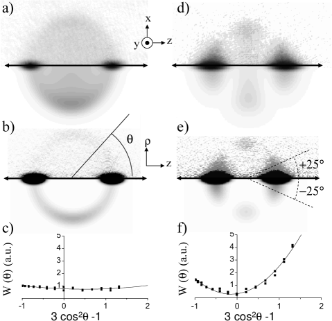
Figure 1: a) Optical density of the scattering halo of two ⁸⁷Rb condensates for collision energy $E/k_{B}=138(4)\,\mu$K, measured 2.4 ms after the collision (upper half: measured; lower half: calculated Calculation ); b) radial density distribution obtained after tomography transformation of image-a (upper half: measured; lower half: calculated Calculation ); c) the dots show the angular scattering distribution $W\left(\theta\right)$ obtained after binning plot b, the line is the best parabolic fit. d,e,f) As in plots a,b,c, but measured 0.5 ms after a collision at 1230(40) $\mu$K. The field of view of the images is $\sim 1\times 1$mm².

As the atoms are scattered by a central field, the scattering pattern must be axially symmetric around the (horizontal) scattering axis ($z$-axis). As pointed out by the Weizmann group Ozeri-02 , this allows a computerized tomography transformation Born-Wolf to reconstruct the radial density distribution of the halo in cylindrical coordinates,

$$n\left(\rho\mathbf{,}z\right)=\frac{1}{4\pi}\int_{-\infty}^{\infty}\tilde{n}_{2}\left(\kappa_{x},z\right)J_{0}\left(\kappa_{x}\rho\right)\left|\kappa_{x}\right|d\kappa_{x}.$$ (1)

Here $\rho=\left(x^{2}+y^{2}\right)^{1/2}$, $\tilde{n}_{2}\left(\kappa_{x},z\right)$ is the 1D Fourier transform along the $x$-direction of the optical density with respect to $z$, and $J_{0}\left(\varrho\right)$ is the zero-order Bessel function. The transformed plots corresponding to the images of Fig. 1a,d are shown as Fig. 1b,e respectively.

To obtain the angular scattering distribution $W(\theta)$ the tomography pictures are binned in 40 discrete angular sectors. For gas clouds much smaller than the diameter of the halo, $W\left(\theta\right)$ is directly proportional to the differential cross section $\sigma\left(\theta\right)=2\pi\left|f\left(\theta\right)+f\left(\pi-\theta\right)\right|^{2}$. Here, the Bose-symmetrized scattering amplitude is given by a summation over the even partial waves, $f\left(\theta\right)+f\left(\pi-\theta\right)=(2/k)\sum_{l=even}(2l+1)e^{i\eta_{l}}P_{l}(\cos\theta)\sin\eta_{l}$. Note that unlike in the total elastic cross section ($\sigma=\int_{0}^{\pi/2}\sigma\left(\theta\right)\sin\theta d\theta=(8\pi/k^{2})\sum_{l=even}(2l+1)\sin^{2}\eta_{l}$), the interference between the partial waves is prominent in the differential cross section. Given the small collision energy in our experiments, only the $s$- and $d$-wave scattering amplitudes contribute, $f_{s}\left(\theta\right)+f_{s}\left(\pi-\theta\right)=(2/k)e^{i\eta_{0}}\sin\eta_{0}$ and $f_{d}\left(\theta\right)+f_{d}\left(\pi-\theta\right)=(2/k)(5/2)e^{i\eta_{2}}\left(3\cos^{2}\theta-1\right)\sin\eta_{2}$. Therefore the differential cross section is given by

$$\sigma(\theta)=\frac{8\pi}{k^{2}}\sin^{2}\eta_{0}\left[1+5\cos(\eta_{0}-\eta_{2})u+\frac{25}{4}u^{2}\right],$$ (2)

where $u\equiv\left(\sin\eta_{2}/\sin\eta_{0}\right)\left(3\cos^{2}\theta-1\right)$.

To obtain the phase shifts, we plot the measured angular distribution $W\left(\theta\right)$ as a function of $\left(3\cos^{2}\theta-1\right)$ as suggested by Eq. (2). The results for Fig. 1a and Fig. 1d are shown as the solid dots in Fig. 1c and Fig. 1f, respectively. A parabolic fit to $W\left(\theta\right)$ directly yields a pair $(\eta_{0}^{\exp}(k),\eta_{2}^{\exp}(k))$ of asymptotic phase shifts (defined modulo $\pi$) corresponding to the two partial waves involved PhaseShiftIndependent . The absolute value of $W\left(\theta\right)$ depends on quantities that are hard to measure accurately (like the atom number) so we leave it out of consideration. We rather emphasize that the measurement of the phase shifts is a complete determination of the (complex) $s$- and $d$-wave scattering amplitudes at a given energy.

The radial wavefunctions corresponding to scattering at different (low) collision energies and different (low) angular momenta should all be in phase at small interatomic distances AccumulatedPhase . This so-called accumulated phase common to all low-energy wavefunctions can be extracted from the full data set $\{(\eta_{0}^{\exp}(k),\eta_{2}^{\exp}(k))\}$ mentioned above. In practice, we use the experimental phase shifts $\eta_{0}^{\exp}(k)$ and $\eta_{2}^{\exp}(k)$ as boundary conditions to integrate inwards - for given $E$ and $l$ - the Schrödinger equation $\hbar^{2}d^{2}\chi(r)/dr^{2}+p^{2}(r)\chi(r)=0$, and obtain the radial wavefunctions $\chi(r)/r$ down to radius $r_{in}=20\,a_{0}$. Here, $p^{2}(r)=m\left(E-V(r)\right)-\hbar^{2}l(l+1)/r^{2}$, where $V(r)\simeq-C_{6}/r^{6}$ is the tail of the interaction potential. At radius $20\,a_{0}$, the motion of the atoms is quasi-classical and the accumulated phase can be written as $\Phi(r)\simeq\arctan\left[p(r)/(\hbar\,\partial\ln\chi/\partial r)\right]$.

Figure 2: a) $d$-wave and b) $s$-wave phase shifts versus collision energy in $\mu$K. The circles are the results of the parabolic fit of $W(\theta)$ for individual images. The full black lines is calculated from the accumulated phase $\Phi_{\mathrm{opt}}$ optimized from all data points. The grey lines show the influence of the uncertainty of $\pm\,\pi\times 0.025$ on $\Phi_{\mathrm{opt}}$. (The vertical dotted line indicates the condition $\eta_{0}=\eta_{2}$). $s-d$ interference is only observed in the gray areas. The first $s$-wave Ramsauer-Townsend minimum is found at $E_{RT}=2.1(2)$ mK.

The distance $20\,a_{0}$ is small enough InnerRadius for $\Phi(r_{in})$ to be highly insensitive to small variations in $E$ or $l$ AccumulatedPhase and large enough that the $-C_{6}/r^{6}$ part of the interaction potential is dominant over the full range of integration. With a least-square method we establish the best value $\Phi_{\mathrm{opt}}(r_{in})=1.34\pm\pi\times 0.025$ for the accumulated phase at $20\,a_{0}$ LeastSquare . Here the error bar reflects the experimental accuracy and not the systematic error related to the choice of $C_{6}$, the latter being of less relevance as discussed below. Interestingly, the $d$-wave scattering resonance Boesten-97 results in a sudden variation of $\eta_{2}^{\exp}$ with the collision energy in the vicinity of that resonance (see Fig.  2a). This imposes a stringent condition on the optimization of $\Phi_{\mathrm{opt}}$ and constrains its uncertainty.

Once $\Phi_{\mathrm{opt}}$ has been established, one can use it as a boundary condition to integrate the Schrödinger equation outwards and compute $\eta_{l}(k)$ for any desired (low) value of $k$ and $l$. Fig. 2 shows the resulting phase shifts for collision energies up to $5$ mK g-wave . The first Ramsauer-Townsend minimum RamsauerMinimum in the $s$-wave cross section is found at collision energy $E_{RT}/k_{B}=2.1(2)$ mK. The solid dots represent the $\eta_{l}^{\exp}(k_{i})$ obtained from the parabolic fit of $W\left(\theta\right)$ from individual images. The three open circles correspond to measurements for which the sign of the phase shifts could not be established Signs . Refinements to the present data analysis may include the occurrence of multiple scattering as well as the influence of the spatial extension of the colliding clouds taking into account the non condensed fraction.

Figure 3: s-wave (dashed line), d-wave (dotted line) and total (full black line) elastic cross sections (in cm²) versus collision energy (in $\mu$K), computed from the optimized accumulated phase $\Phi_{\mathrm{opt}}$ as determined in this work. The gray lines are the total elastic cross sections, obtained from $\Phi_{\mathrm{opt}}\pm\pi\times 0.025$.

Knowing the phase shifts, we can infer all the low-energy scattering properties. Our results for the elastic scattering cross section are shown in Fig. 3. The (asymmetric) $d$-wave resonance emerges pronouncedly at $300(70)\ \mu$K with an approximate width of $150\;\mu$K (FWHM). Most importantly, the scattering length follows from the $k\rightarrow 0$ limiting behavior, $\eta_{0}(k\rightarrow 0)=-ka$. We find $a=+102(6)\,a_{0}$, whereas the state-of-the-art value is $a=98.99(2)\,a_{0}$ Kempen-02 .

Comparison with the precision determinations Marte ; Kempen-02 shows that our method readily yields fairly accurate results, relying only on input of the $C_{6}$ coefficient. We used the value $C_{6}=4.698(4)\times 10^{3}\;$a.u. Kempen-02 . In the present case, one does not need to know $C_{6}$ to this accuracy. Increasing $C_{6}$ by $10\%$ results in a 1 $\%$-change of the scattering length. Clearly, the systematic error in $\Phi_{\mathrm{opt}}$ accumulated by integrating the Schrödinger equation inward with a wrong $C_{6}$ largely cancels when integrating back outward. However, in the case of a $s$-wave resonance other atomic species may reveal a stronger influence of $C_{6}$ on the calculated scattering length. Simple numerical simulations show that the value of $C_{6}$ becomes critical only when the (virtual) least-bound state in the interaction potential has an extremely small (virtual) binding energy (less than $10^{-2}$ level spacing). Hence our method should remain accurate in almost any case.

This method can therefore be applied to other bosonic or fermionic atomic species, provided the gases can be cooled and accelerated in such a way that the lowest-order partial-wave interference can be observed with good energy resolution. We speculate that the accuracy of the method can be strongly improved by turning to smaller optical-density clouds and fluorescence detection. It will enable higher collision energies and observation of higher-order partial-wave interference. The use of more dilute clouds and longer expansion times will also eliminate multiple-scattering effects and finite-size convolution broadening of the interference pattern. Finally it will enable precision measurements of the scattered fraction, which in the case of ⁸⁷Rb will allow us to pinpoint the location of the $d$-wave resonance to an accuracy of $10\,\mu$K or better. In combination with state-of-the-art theory such improvements are likely to turn our approach into a true precision method.

Similar experiments were reported during the final stage of completion of this Letter Kiwis .

The authors acknowledge valuable discussions with S. Kokkelmans, D. Petrov, G. Shlyapnikov, S. Gensemer and B. Verhaar. This work is part of the research programme of the ‘Stichting voor Fundamenteel Onderzoek der Materie (FOM), supported by the ‘Nederlandse organisatie voor Wetenschappelijk Onderzoek (NWO)’. JL acknowledges support from a Marie Curie Intra-European Fellowship (MEIF-CT-2003-501578).

References

- (1) See e.g. L. Pitaevskii and S. Stringari, Bose-Einstein condensation, Clarendon Press, Oxford 2003; C.J. Pethick and H. Smith, Bose-Einstein condensation in dilute gases, Cambridge University Press, Cambridge 2002.
- (2) D.S. Petrov, C. Salomon and G.V. Shlyapnikov, cond-mat0309010.
- (3) P.O. Fedichev, M.W. Reynolds and G.V. Shlyapnikov, Phys. Rev. Lett. 77, 2921 (1996).
- (4) J. Weiner, V.S. Bagnato, S. Zilio, and P.S. Julienne, Rev. Mod. Phys. 71,1 (1999).
- (5) D.G. Friend and R.D. Etters, J. Low Temp. Phys. 39, 409 (1980); Y.H. Uang and W.C. Stwalley, J. de Phys.41, C7-33 (1980).
- (6) C. R. Monroe et al., Phys. Rev. Lett. 70, 414 (1993); S. D. Gensemer et al., Phys. Rev. Lett., 87, 173201 (2001).
- (7) G. Ferrari et al., Phys. Rev. Lett. 89, 53202 (2002); P. Schmidt et al., Phys. Rev. Lett. 91, 193201 (2003).
- (8) D. Heinzen, in: Proceedings of the international School of Physics - Enrico Fermi, M. Inguscio, S. Stringari and C. Wieman (Eds.), IOS Press, Amsterdam 1999.
- (9) C. Samuelis et al., Phys. Rev. A 63, 12710 (2001).
- (10) C. Chin, V. Vuletic, A. J. Kerman, and S. Chu, Phys. Rev. Lett. 85, 2717 (2000); P. J. Leo, C. J. Williams, and P. S. Julienne, Phys. Rev. Lett. 85, 2721 (2002).
- (11) A. Marte et al., Phys. Rev. Lett., 89, 283202 (2002).
- (12) M. Born and E. Wolf, Principles of Optics, 7th (expanded) Edition, Cambridge University Press, Cambridge 1999.
- (13) B. Verhaar, K. Gibble, and S. Chu, Phys. Rev. A 48, R3429 (1993); G.F. Gribakin and V.V. Flambaum, Phys. Rev. A 48, 546 (1993).
- (14) R. Legere and K. Gibble, Phys. Rev. Lett. 81, 5780 (1998).
- (15) H.M.J.M. Boesten, C.C. Tsai, J.R. Gardner, D. J. Heinzen, B.J. Verhaar, Phys. Rev. A 55, 636 (1997).
- (16) E.G.M. van Kempen, S.J.J.M.F. Kokkelmans, D.J. Heinzen, and B.J. Verhaar, Phys. Rev. Lett. 88, 93201 (2002); B.J. Verhaar and S.J.J.M.F. Kokkelmans, private communications.
- (17) T.G. Tiecke et al., J. Opt. B 5, S119 (2003); see also N. R. Thomas, A. C. Wilson, and C. J. Foot, Phys. Rev. A 65, 063406 (2002).
- (18) A. P. Chikkatur et al., Phys. Rev. Lett., 85, 483 (2000); J. M. Vogels, K. Xu, and W. Ketterle, Phys. Rev. Lett. 89, 20401 (2002).
- (19) Based on the phase shifts reported in this Letter.
- (20) R. Ozeri, J. Steinhauer, N. Katz, and N. Davidson, Phys. Rev. Lett., 88, 220401, (2002).
- (21) This procedure breaks down in the marginal case , where the expression in the square brackets in Eq. (2) becomes phase-shift independent.
- (22) We checked that, within the range , the exact choice of the inner radius of the integration interval is of no influence for the results presented in this Letter.
- (23) The determination of is done by minimizing , where N is the number of data points, and the are the phase shifts computed from .
- (24) The -wave phase shift can also be computed from the same , but the error made by assuming a constant accumulated phase increases like , and the resulting -wave would be accordingly less accurate.
- (25) Ramsauer-Townsend minima are observed around collision energies where a phase shift crosses zero (see Fig. 2).
- (26) Since Eq. (2) is unchanged under reversal of the sign of both and , the result of the parabolic fit is not unique. We eliminate this ambiguity by comparing the difference in accumulated phases obtained for and with that obtained for and . We find that in almost all cases, this difference - which should be vanishingly small - is much larger for one choice of signs than for the other. We conclude that the correct sign for a pair is the one for which the difference between the accumulated phases is the smallest. In all but three cases (at the same collision energy), this criterium is conclusive. These three measurements (the open circles in Fig. 2) are left out of the procedure used to compute . In hindsight they turn out to correspond to the marginal case mentioned in PhaseShiftIndependent .
- (27) N. R. Thomas, N. Kjærgaard, P. S. Julienne, and A. C. Wilson, cond-mat/0405544.