Positional Disorder, Spin-Orbit Coupling and Frustration in ${\rm Ga}_{1-x}{\rm Mn}_{x}{\rm As}$

Abstract

We study the magnetic properties of metallic ${\rm Ga}_{1-x}{\rm Mn}_{x}{\rm As}$. We calculate the effective RKKY interaction between Mn spins using several realistic models for the valence band structure of GaAs. We also study the effect of positional disorder of the Mn on the magnetic properties. We find that the interaction between two Mn spins is anisotropic due to spin-orbit coupling both within the so-called spherical approximation and in the more realistic six band model. The spherical approximation strongly overestimates this anisotropy, especially for short distances between Mn ions. Using the obtained effective Hamiltonian we carry out Monte Carlo simulations of finite and zero temperature magnetization and find that, due to orientational frustration of the spins, non-collinear states appear in both valence band approximations for disordered, uncorrelated Mn impurities in the small concentration regime. Introducing correlations among the substitutional Mn positions or increasing the Mn concentration leads to an increase in the remnant magnetization at zero temperature and an almost fully polarized ferromagnetic state.

I Introduction

Recently, there has been a surge of interest in the more than 30 year old field of diluted magnetic semiconductorsrev that has been largely motivated by potential application of these materials in spin-based computationDiVincenzo (1995); Nielson and Chuang (2000); Awschalom et al. (2002); Zutic et al. (2004) devices. In particular, the discovery of ferromagnetism in low-temperature molecular beam epitaxy (MBE) grown ${\rm Ga}_{1-x}{\rm Mn}_{x}{\rm As}$ has generated renewed interest. In this material Curie temperatures as high as $T_{c}\approx 160{\rm K}$ have been observed.Edmonds et al. (2004)

It is typically rather difficult to dissolve magnetic impurities in a semiconductor using conventional MBE techniques, because the magnetic ions usually tend to segregate from the host. As a result, these conventionally produced magnetic semiconductors often exhibit spin glass physics at low temperatures and other, undesirable, “clustering” effects. Recently Ohno achieved the key breakthrough,Ohno et al. (1996) by growing ${\rm Ga}_{1-x}{\rm Mn}_{x}{\rm As}$ at close to room temperature, which minimized Mn positional relaxation during the growth process, and resulted in a material with intrinsic ferromagnetic properties, with a Curie temperature $T_{C}\sim 110{\rm K}$.

Post-growth annealing of the samples was shown to induce changes both in the lattice and positional defectsPotashnik et al. (2001); Edmonds et al. (2004); Yu et al. (2002a); Hayashi et al. (2001) as well as in the hole concentration.Yu et al. (2002b); Sorenson et al. (2003) Properties such as magnetization and Curie temperature, were found to depend very sensitively on details of the post-growth annealing protocolOhno (1999); Potashnik et al. (2001); Edmonds et al. (2002); Ku et al. (2003). In particular, the measured $T=0$ temperature magnetization has been found to be much less than one expected based on the nominal concentration of Mn ions.Potashnik et al. (2003) The remnant magnetization and the Curie temperature $T_{C}$ were both found to increase upon annealing, but the magnetization reached only about half of the expected value even in the case of optimally annealed samples Potashnik et al. (2001, 2003, 2002). According to recent experimental results, much of the missing magnetization is probably due to interstitial Mn ions, which compensate valence band holes,Edmonds et al. (2004); Yu et al. (2002a) and, presumably, also bind antiferromagnetically to substitutional Mn ions.Bergqvist et al. (2003) As a result, the nominal concentration of Mn ions, $x$, is usually substantially larger than the concentration of active Mn ions (participating in the ferromagnetism), $x_{\rm active}$, which is larger than the concentration of mobile holes in the valence band (or possibly impurity band Fiete et al. (2003); Berciu and Bhatt (2001)), $c=x_{\rm active}\;f$, with $f<1$ the hole fraction. [In the remainder of this paper - unless explicitly noted otherwise - we present the results in terms of the active Mn concentration: $x\equiv x_{\rm active}$.] However, especially for samples with a lower doping level and/or shorter annealing times, even this substantial difference in active and nominal Mn concentration seems to be insufficient to explain the total amount of lost of magnetization: In some of these samples the remnant magnetization can be substantially increased by a relatively small magnetic field, clearly hinting at a non-collinear magnetic state.Potashnik et al. (2003)

Many of the properties of ${\rm Ga}_{1-x}{\rm Mn}_{x}{\rm As}$ depend crucially on defects, and understanding these defects is currently a subject of intense research.Tim (a); Edmonds et al. (2004); Bergqvist et al. (2003); Blinowski and Kacman (2003); Korzhavyi et al. (2002); Yu et al. (2002a); Máca and Masek (2002) ${\rm Ga}_{1-x}{\rm Mn}_{x}{\rm As}$ is a complicated material: Besides containing many defects of unknown origin, it is very disordered, close to a localization transition with a mean free path of the order of the Mn-Mn distance, has a complicated band structure, has strong spin-orbit coupling and has a large exchange coupling between the localized Mn spins and the valence holes. It is therefore almost impossible to study this material without making some approximations.

As pointed out in Ref. [Zaránd and Jankó, 2002], spin-orbit coupling can induce frustration and non-collinear states in a disordered magnet. In this paper, we study the effect of spin-orbit coupling in the metallic limit (i.e., holes are assumed to reside entirely in the valence bands of GaAs) of ${\rm Ga}_{1-x}{\rm Mn}_{x}{\rm As}$, and study how it may influence the structure of the ferromagnetic state. To this purpose, we will follow the route outlined in Ref. [Zaránd and Jankó, 2002] and compute the effective interaction between the spin of two substitutional Mn impurities by doing perturbation theory in the exchange interaction (RKKY interaction). It is important to note that other mechanisms also exist that could lead to a non-collinear state.Schliemann (2003); Schliemann and MacDonald (2002) Recently, several studies of RKKY models of Mn spin-spin interactions in GaMnAsZaránd and Jankó (2002); D. J. Priour et al. (2004); Brey and Gómez-Santos (2003); Singh et al. (2003); Bouzerar et al. (2003); Tim (b) have been reported, but these studies have not investigated in detail the effects of positional disorder on the magnetic properties using realistic band structure models.

In this work, we neglect the effect of other defects and the strong scattering potential on the charged substitutional Mn impurities. This approximation - which is quite common in the literatureKönig et al. (2000); Abolfath et al. (2001) - is expected to provide qualitatively reliable results relatively deep in the metallic state, far away from the localization transition, where screening is expected to reduce the effets of charged impurities. Quantitative agreement with experiment will require treating both charging effects and defect correlations in a realistic way.Timm et al. (2002); Tim (a) Furthermore, scattering from charged impurities becomes even more important in the dilute limit, and is ultimately responsible for the localization transition that occurs at small concentrations. In this dilute limit, the strong potential scattering off Mn impurities can be treated nonperturbatively, and results similar to those reported here are obtained.Fiete et al. (2003); Paw

In the absence of disorder the top of the valence band of ${\rm Ga}{\rm As}$ can be described within the framework of $k\cdot p$ perturbation theory, which also accounts for the spin-orbit coupling in this material, and gives a good description of the band structure around the $\Gamma$ point. In particular, we study two different forms of the $k\cdot p$ perturbation theory. First we study the effective spin-spin interaction within a simplified version of the four band model, the so-called spherical model,Baldereschi and Lipari (1973) where only the topmost four spin $j=3/2$ bands are kept and the distortion of the spherical Fermi surface is neglected. In this case analytical results can be obtained for the effective Mn spin-spin interaction.Zaránd and Jankó (2002) Then we study the Mn spin-spin interaction using a six band modelAbolfath et al. (2001); König et al. (2001) (Kohn-Luttinger HamiltonianKohn and Luttinger (1955)), where the spin-orbit split $j=1/2$ band is also taken into account. In the latter case it is not possible to evaluate the interaction kernel analytically, and one must resort to numerics.

Although we find in both calculations a strong spin-orbit induced anisotropy in the spin-spin interaction for typical Mn-Mn distances, the spherical model largely overestimates the size of the anisotropy for small distances. We find it especially instructive to discuss this result in comparison with those published recently in a nice and intriguing paper by Brey and Gómez-Santos. Brey and Gómez-Santos (2003) While our result agrees qualitatively with the one obtained in Ref.[Brey and Gómez-Santos, 2003], on a quantitative level it is completely different. Brey and Gómez-Santos estimated that the largest value of the anisotropy is of the order of $\sim 10^{-4}$. In contrast, in the present calculation we find that the smallest value of the anisotropy is around $1\%$ for nearest neighbor Mn ions at a distance of $\sim 2.5\AA$, and it increases continuously with distance, until it reaches a value of the order of $\sim 20\;\%$ for typical Mn-Mn distances. These numbers roughly agree with the results obtained in the very dilute limit for a ${\rm Mn}_{2}$ “molecule” within the six band model.Paw

There are basically two reasons for the discrepancy between the two results:
(1) Presumably to avoid convergence problems, Brey and Gómez-Santos introduced a short distance cut-off $a_{0}$, and replaced the exchange interaction between the Mn core spins and valence holes by a non-local interaction. The cut-off scheme they introduced, however, is not compatible with the general structure of the exchange interaction derived in the microscopic theory of quantum impurities.Hewson (1997) As we discuss in detail in Sec. III, the corresponding momentum cut-off introduced should not be smaller than $\sim 2k_{F}$, the typical momentum transfer during backscattering. Unfortunately, the cut-off $a_{0}=4\AA$ used in Ref. [Brey and Gómez-Santos, 2003] did not satisfy this criterion, and as a consequence, the results of Ref. [Brey and Gómez-Santos, 2003] showed a very strong dependence on $a_{0}$: In particular, for somewhat smaller values of $a_{0}=2.42\AA$ Brey and Gómez-Santos found an anisotropy of a few percent, which roughly agrees with the one we find ($\approx$ 1 %) within a cut-off scheme compatible with the general theory of magnetic interactions for nearest neighbor Mn ions. The strong dependence of the Brey-Gómez-Santos result on the cut-off parameter was also pointed out and questioned recently by Timm and MacDonald in Ref.[Tim, b]. We emphasize that with our cut-off scheme the anisotropy depends only weakly on the value of $a_{0}$.
(2) Secondly, in Ref. [Brey and Gómez-Santos, 2003] it has been assumed that the anisotropy is largest for the shortest Mn-Mn separations. However, for hole concentrations $p\leq 3\ {\rm nm}^{-3}$ one actually expects on general grounds that the asymptotic form of the RKKY interaction is reasonably well-approximated within the four band model, which assumes infinite spin-orbit splitting $\Delta_{SO}$, and that the anisotropy increases with Mn-Mn separation. This is indeed supported by our numerical results: For the very small separations for which Brey and G’omez-Santos carried out their calculations we indeed find only a $\sim 1\%$ anisotropy, while for typical Mn-Mn separations we find a rather large anisotropy of the order of $\sim 20\%$.

Having the interaction kernels at hand, we considered a distribution of Mn ions and carried out finite temperature Monte Carlo simulations to characterize the magnetic properties of the system. At present, it is unclear from the experiments to what extent the positions of substitutional, magnetically active Mn are correlated during the growth process. In order to gain insight into how Mn positional correlations may affect the magnetic properties of a material like GaMnAs, we studied the dependence of the Curie temperature, the saturation magnetization, the shape of the magnetization curve and the ground state spin distribution on Mn positional correlations. These correlations were introduced by allowing repulsive interactions between the Mn ions and relaxing them through a zero temperature Monte Carlo Metropolis algorithm in a way similar to Ref. [Timm et al., 2002]. We started the simulations from a set of completely uncorrelated initial Mn positions, and allowed the substitutional Mn ions to move. We then studied the magnetic properties of the spin system as a function of the Mn positional relaxation time, including the completely uncorrelated configuration.

Our main results are as follows: Within the spherical approximation we find a strongly disordered (non-collinear) ferromagnetic ground state for unrelaxed Mn positions, where the ground state magnetization can be reduced by as much as $\sim 50\%$ with respect to its saturation value. Upon relaxing the Mn positions, however, the remnant magnetization increases, and for a fully relaxed lattice one may recover as much as $95\%$ of the saturation value. In contrast to our earlier expectations,Zaránd and Jankó (2002) the obtained non-collinear state is not a spin-glass: Although a finite system displays hysteresis, the coercive field we compute decreases with system size, implying that the hysteresis vanishes in the infinite system size limit. The frustration effects found within the spherical model are very sensitive to the hole fraction $f$ characterizing the degree of compensation, and become more pronounced for larger hole fractions.

Spin-orbit coupling induced anisotropy does not have such a dramatic effect if we use the kernel obtained within the six-band model. For a substitutional Mn concentration of $x=3\%$, hole fraction $f=0.4$, and unrelaxed Mn spins we find that the magnetization is reduced by $\sim 5\%$, relative to the fully polarized state, corresponding to a typical non-collinear angle of the order of $\theta\sim 16$ degrees. This non-collinearity is, however, almost completely suppressed if we let the Mn positions relax using the Monte Carlo algorithm mentioned above. By increasing the substitutional Mn concentration to $x=5\%$ the ground state becomes almost fully collinear even without relaxing the Mn positions. The results do not depend too strongly on the level of compensation (hole fraction). Our results also indicate that anisotropy effects may be more important for smaller Mn concentrations.Fiete et al. (2003)

We emphasize again that the concentration $x$ above denotes the concentration of active Mn ions, i.e. the concentration of those Mn ions that participate in the formation of the ferromagnetic state. Due to compensation effects induced by interstitial Mn impurities, $x$ is usually much less than the nominal concentration of Mn ions. In fact, samples with a nominal concentration of $5\%$ may easily have an active Mn concentration in the range $x<0.02\;-\;0.03$. In this concentration range the impurity band approach of Refs. [Berciu and Bhatt, 2001] and [Fiete et al., 2003] may be more appropriate.

In agreement with the results of Ref. [Berciu and Bhatt, 2004], we also find that in all cases $T_{C}$ decreases as we relax the Mn impurities, irrespective of the specific form of effective interaction used, and $M(T)$ becomes more mean-field like at the same time.

This paper is organized as follows. In Sec. II we present the RKKY calculation within the Baldereschi-Lipari spherical approximation for the effective interaction between two Mn spins. Several of the most technical details and lengthy expressions have been relegated to Appendices A and B. Sec. III is devoted to the computation of the effective Mn spin-spin interaction within the full six band model. In Sec. IV we discuss the results of classical Monte Carlo calculations for the magnetization, the ground state spin distributions, the Curie temperature and the dependence of these quantities on positional disorder and hole concentration using the effective spin-spin interactions computed in Sections II and III. Finally, in Sec. V we summarize our main conclusions.

II Effective Mn Spin-Spin Interaction in the Spherical Approximation

In the present section, we study the effective RKKY interaction between two Mn impurities, by using the so-called spherical approximation to describe the valence band hole fluid. The top of the valence band of GaAs consists of six $p$-bands. Four of these bands become fourfold degenerate at the $\Gamma$ point and have spin $j=3/2$ character, while the other two are split off by $\Delta_{SO}\approx 0.34\;{\rm eV}$ and have spin $j=1/2$ character.Blakemore (1982)

The spherical approximation consists of setting the spin-orbit splitting $\Delta_{SO}$ to infinity, keeping only the spin $j=3/2$ bands, neglecting the warping of the Fermi surface due to the cubic symmetry of the crystal, and approximating the dispersion of the holes by the following expression:Baldereschi and Lipari (1973)

$$H_{\rm sp}={\gamma_{1}\over 2m}\left(p^{2}-\nu\sum_{\alpha,\beta}J_{\alpha\beta}p_{\alpha\beta}\right)\;.$$ (1)

Here $J_{\alpha\beta}={1\over 2}(j_{\alpha}j_{\beta}+j_{\beta}j_{\alpha})-{1\over 3}\delta_{\alpha\beta}{\rm Tr}\{j_{\alpha}j_{\beta}\}$ is the quadrupolar angular momentum of the holes. The linear momentum tensor of the holes $p_{\alpha\beta}$ is defined likewise. The coupling $\nu=(6\gamma_{3}+4\gamma_{2})/5\gamma_{1}\approx 0.77$ characterizes the strength of the effective spin-orbit coupling within the $j=3/2$ band, and the $\gamma_{i}$’s are the so-called Luttinger parametersKohn and Luttinger (1955), characterizing the band structure of GaAs. Physically the parameter $\nu$ describes how the spin of a $j=3/2$ valence hole couples to its orbital motion.

The advantage of the spherical approximation, Eq. (1), is that it makes it possible to obtain analytical results while it gives a realistic description of the top of the valence band. As we will see, this latter fact is somewhat misleading: While providing a qualitatively correct description of the valence bands of Ga_1-xMn_xAs, it gives quantitatively incorrect results for the RKKY interaction between two local spins.

In GaMnAs subsitutional Mn ions are believed to be in a ${\rm Mn}^{2+}$ configurarationLinnarson et al. (1997); Szczytko et al. (1999); Okabayashi et al. (1998) thereby behaving as a negatively charged scatterer and having a core spin $S=5/2$. This core spin then couples to the spin of the valence hole fluid through an exchange interaction that, for a single Mn ion, takes the following form within the spherical approximation:

$$H_{\rm int}({\bf R})=G{\bf S\cdot j(R)}\;,$$ (2)

where ${\bf j(R)}$ denotes the valence holes’ spin density, at the location of the Mn ion, ${\bf R}$, and $G>0$ is an antiferromagnetic coupling.

To proceed let us first show that the eigenstates of $H_{\rm sp}$ are chiral, i.e., that the spin is quantized along the direction of propagation. First we note that $H_{\rm sp}$ for holes propagating along the $z-$direction is easily diagonalized: ${\bf p}=(0,0,p_{z})$ so that

$$\sum_{\alpha,\beta}J_{\alpha\beta}p_{\alpha\beta} = \left(j_{z}^{2}-\frac{j(j+1)}{3}\right)p_{z}^{2}=\pm p_{z}^{2}\;.$$

Thus, for holes moving in the $z-$direction,

$$H_{\rm sp}={\gamma_{1}p_{z}^{2}\over 2m}(1\pm\nu)\;,$$ (3)

with the plus and minus signs standing for $j_{z}=\pm 1/2$ and $j_{z}=\pm 3/2$, respectively. This defines the light hole mass, $m_{l}=\frac{m}{\gamma_{1}(1+\nu)}\approx 0.07m$ and the heavy hole mass $m_{h}=\frac{m}{\gamma_{1}(1-\nu)}\approx 0.5m$ where $m$ is the bare electron mass. For holes propagating in a general direction, the wave function can be constructed by spin 3/2 rotations so that $\mu={\bf j}\cdot{\bf\hat{k}}=\pm 3/2$ for heavy holes and $\pm 1/2$ for light holes propagating along direction $\hat{\bf k}$.

The kinetic energy $H_{\rm sp}$ greatly simplifies in the basis of these chiral states, and takes the following form in second quantized formalism:

$$\hat{H}_{\rm sp}=\sum_{{\bf k},\mu}{k^{2}\over 2m_{\mu}}c^{\dagger}_{{\bf k}\mu}c_{{\bf k}\mu}\;.$$ (4)

Here $c^{\dagger}_{{\bf k}\mu}$ denotes the creation operator of a hole with wavevector ${\bf k}$ and spin projection $\mu$ along $\hat{\bf k}$. Diagonalizing $\hat{H}_{\rm sp}$, however, produces a strongly momentum dependent carrier-impurity interaction:

$$\hat{H}_{\rm int}={G\over V}\sum_{{\bf k},{\bf k^{\prime}}}\sum_{\alpha,\mu,\mu^{\prime}}S^{\alpha}c^{\dagger}_{{\bf k}\mu}j^{\alpha}_{\mu\mu^{\prime}}(\hat{\bf k},\hat{\bf k^{\prime}})c_{{\bf k^{\prime}}\mu^{\prime}}e^{-i{\bf(k-k^{\prime})R}}\;.$$ (5)

Here $j^{\alpha}_{\mu\mu^{\prime}}(\hat{\bf k},\hat{\bf k^{\prime}})\equiv\sum_{j,j^{\prime}}D^{\dagger}_{\mu j}(\hat{\bf k})j^{\alpha}_{jj^{\prime}}D_{j^{\prime}\mu^{\prime}}(\hat{\bf k^{\prime}})$ where $D(\hat{\bf k})$ is the spin 3/2 rotation matrix and V is the volume of the sample. The rotation matricies are defined here in the usual way as $D_{j\mu}(\hat{\bf k})=[e^{-i{\hat{j}^{z}\phi\over\hbar}}e^{-i{\hat{j}^{y}\theta\over\hbar}}]_{j\mu}$, where $\phi$ and $\theta$ are the usual azimuthal and polar angle of the direction ${\bf\hat{k}}=(\sin\theta\cos\phi,\;\sin\theta\sin\phi,\;\cos\theta)$.

Having diagonalized $H_{\rm sp}$, we now consider two Mn ions at positions ${\bf R}$ and the origin, do perturbation theory in the exchange coupling $G$ and compute the RKKY interaction between two Mn spins.Yosida (1996) The first order correction to the single particle eigenstate $|{\bf k},\mu\rangle_{0}$ of $H_{\rm sp}$ is given by

$$|{\bf k},\mu\rangle^{\prime}=|{\bf k},\mu\rangle_{0}-{G\over V}\sum_{\alpha,{\bf k^{\prime}},\mu^{\prime}}{j^{\alpha}_{\mu\mu^{\prime}}(\hat{\bf k},\hat{\bf k^{\prime}})S^{\alpha}\over\epsilon_{{\bf k^{\prime}}\mu^{\prime}}-\epsilon_{{\bf k}\mu}}|{\bf k^{\prime}},\mu^{\prime}\rangle_{0}\;,$$ (6)

where the sum is over all states except for $|{\bf k},\mu\rangle_{0}$, and $\epsilon_{{\bf k}\mu}=k^{2}/2m_{\mu}$. With these single particle states in hand, we can then compute the shift of the ground state energy as:

$$H_{\rm RKKY} = -2\left({G\over V}\right)^{2}\sum_{\alpha\beta}{\bf S_{R}^{\alpha}S_{0}^{\beta}}$$

$$\times\sum_{\scriptstyle{\bf k},\mu\atop\scriptstyle{\bf k^{\prime}}\mu^{\prime}}{1\over\epsilon_{{\bf k^{\prime}}\mu^{\prime}}-\epsilon_{{\bf k}\mu}}\left(e^{i{\bf(k^{\prime}-k)R}}j^{\beta}_{\mu\mu^{\prime}}j^{\alpha}_{\mu^{\prime}\mu}+c.c.\right)\;,$$

where we have dropped a piece of the energy independent of relative spin orientations. This equation can be rewritten as

$$H_{\rm RKKY}=-\sum_{\alpha\beta}S^{\alpha}({\bf R})K^{\alpha\beta}({\bf R})S^{\beta}(0)\;,$$ (8)

with an obvious definition of the kernel $K^{\alpha\beta}$. Within the spherical approximation this result further simplifies to

$$H_{\rm eff}=-K_{\rm para}(R){\bf S}_{1}^{||}\cdot{\bf S}_{2}^{||}-K_{\rm perp}(R){\bf S}_{1}^{\perp}\cdot{\bf S}_{2}^{\perp}\;,$$ (9)

where $R=|{\bf R}_{1}-{\bf R}_{2}|$ and ${\bf S}_{i}$ is the Mn spin at position ${\bf R}_{i}$. Here ${\bf S}^{\perp/||}$ refers to the component of the spin perpendicular/parallel to the axis joining them.

The computation of the kernels $K_{||}$ and $K_{\perp}$ is not straightforward even in the case of the spherical approximation. Their explicit expressions and some details about how to obtain them are given in Appendix A. These expressions together with Eq. (9) constitute the main result of this section of the paper.

For more physical transparency, it is worth defining the following rescaled kernel,

$$C_{\rm para/perp}\equiv K_{\rm par/perp}/4\pi\,\epsilon_{F}g_{h}^{2}\;,$$ (10)

where we have defined the dimensionless coupling as $g_{h}=G\varrho_{h}=G{m_{h}^{3/2}\over\sqrt{2}\pi^{2}}\epsilon_{F}^{1/2}$, with $m_{h}$ is the heavy hole mass and $\epsilon_{F}$ is the Fermi energy measured relative to the “top” of the valence band. The positional dependence of $C_{\rm para/perp}$ is shown in Fig. 1, where we also plotted the contribution of the heavy holes, giving the dominant contribution to the interaction kernel. The rather involved explicit expressions for the dimensionless kernel $C(y)$ are given in Appendix A. The asymptotic forms for $y\equiv k_{F,h}R\to 0$ of the kernels $C$ are given by

$$C_{\rm para}^{\rm total}\approx\left[1+\frac{m_{l}^{3/2}}{m_{h}^{3/2}}+\frac{7}{3}\left(\frac{m_{l}}{m_{h}}+\frac{m_{l}^{5/2}}{m_{h}^{5/2}}\right)\right]\frac{1}{2y}=\frac{.698}{y}\;,$$

and

$$C_{\rm para}^{\rm total}\approx\left[1+\frac{m_{l}^{3/2}}{m_{h}^{3/2}}+\frac{2}{3}\left(\frac{m_{l}}{m_{h}}+\frac{m_{l}^{5/2}}{m_{h}^{5/2}}\right)\right]\frac{1}{y}=\frac{1.150}{y}\;,$$

where $m_{l}$ and $m_{h}$ are the light and heavy hole mass defined just below Eq. (3). Specifically, in the limit of $m_{h}\to\infty$ we simply obtain $C_{\rm para}^{\rm heavy}\approx 1/2y$, $C_{\rm perp}^{\rm heavy}\approx 1/y$.

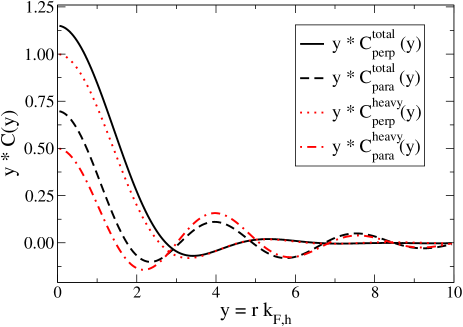
Figure 1: Effective RKKY kernel in the 4-band spherical approximation. The contribution from the heavy hole sector is also shown. At typical Mn-Mn separations the structure of the kernel is very sensitive to the value of the hole fraction $f$. For $f=0.10$ one has $y^{\rm typ}=d^{\rm typ}k_{F,h}=1.6$, while for $f=0.25$ we have $y^{\rm typ}=d^{\rm typ}k_{F,h}=2.2$. In both cases the perpendicular part of the kernel is ferromagnetic, but for $f=0.25$ the parallel component is antiferromagnetic and is comparable in absolute value to the perpendicular component.

Eq. (9), was first obtained in Ref. [Zaránd and Jankó, 2002] using only the heavy hole sector of the valence band structure. There it was shown that Eq. (9) leads to a spin-disordered ground state whose signatures seem to be present in some experiments.Potashnik et al. (2003); Rappoport et al. (2004)

At typical Mn-Mn separations the kernel is very sensitive to the value of the hole fraction. Hole fractions in the range $f=0.10-0.25$ corresponds to ${\rm y^{typ}}_{f=0.10}={\rm d^{typ}}k^{f=0.10}_{F,h}$=1.6 and ${\rm y^{typ}}_{f=0.25}={\rm d^{typ}}k^{f=0.25}_{F,h}$=2.2. In both cases the perpendicular part of the kernel is largest and is ferromagnetic. However, for $f=0.10$ the parallel component is ferromagnetic while for $f=0.25$ the parallel component is antiferromagnetic and of comparable strength to the perpendicular component. The relative size of $K_{\rm perp}$ and $K_{\rm para}$ means that spins prefer to ferromagnetically align perpendicular to the axis joining them for small enough hole concentrations. In general this leads to frustration and non-collinear magnetism.

In Sec. IV we study the finite temperature behavior of the Mn spins using classical Monte Carlo techniques. There we shall assume that the spins behave as classical objects, and we replace Eq. (9) by

$$H_{\rm eff}=-J_{||}(R){\bf\Omega}_{1}^{||}\cdot{\bf\Omega}_{2}^{||}-J_{\perp}(R){\bf\Omega}_{1}^{\perp}\cdot{\bf\Omega}_{2}^{\perp}\;,$$ (11)

where now ${\bf\Omega}_{1}$ and ${\bf\Omega}_{2}$ denote the two unit vectors specifying the direction of the spins, and the exchange couplings are given by

$$J_{||/\perp}=E_{J}\;C_{\rm para/perp}\;,$$ (12)

with the exchange energy defined as

$$E_{J}\equiv S^{2}\;4\pi\,\epsilon_{F}g_{h}^{2}\;.$$ (13)

The precise value of $E_{J}$ depends on the specific value of the unknown coupling $G$ and the hole concentration, $p$, with which it scales as $E_{J}\sim\epsilon_{F}^{2}\sim p^{4/3}$ within the spherical approximation.

III Effective Mn spin-spin interaction in the six band model

In the previous section we studied the effective RKKY interaction between two Mn impurities within the spherical approximation. In the present section we shall study the effective Mn spin-spin interaction by using a more realistic description of the top of the valence band, the so-called six band model, where the Hamiltonian reads

$$H = H_{\rm Lutt}+H_{\rm int}\;,$$ (14)

$$H_{\rm int} = J_{pd}({\bf s}({\bf R}_{1})\cdot{\bf S}_{1}+{\bf s}({\bf R}_{2})\cdot{\bf S}_{2})\;,$$ (15)

with $H_{\rm Lutt}$ being the so-called Kohn-Luttinger Hamiltonian, and ${\bf s}({\bf R})$ the spin density of the holes at position ${\bf R}$. Note that ${\bf s}$ here is not a spin $3/2$ spin object. It is a $6\times 6$ dimensional matrix that represents the spins (1/2) of the holes in the three $p$ channels that constitute the top of the valence band (for an explicit definition see e.g. Ref. [Abolfath et al., 2001]).

The six-band Hamiltonian approximates rather well the band structure and the spin content of the hole states in the vicinity of the $\Gamma$ point of the Brillouin zone. However, it is impossible to evaluate the RKKY interaction analytically using $H_{\rm Lutt}$, and numerical calculations are needed.

To perform the numerical calculations, we followed the procedure of Ref. [Brey and Gómez-Santos, 2003]: We generated a mesh in momentum-space, computed the eigenenergies of $H_{\rm Lutt}$ and the corresponding eigenfunctions, and ordered them according to their energy. We then computed the matrix elements of $H_{\rm int}$ in this basis by treating the spin of the Mn ions classically, and fixing their direction. Next we diagonalized $H_{\rm Lutt}+H_{\rm int}$ to obtain the single particle hole states for this orientation of the spins, while only keeping states below the cut-off energy, $E_{\rm cutoff}$. Finally, we computed the ground state energy of the whole system as a sum of the energy of the occupied single particle states, and thus obtained the ground state energy of the system for a fixed number of holes as a function of the direction of the two spins.

The effective couplings have been extracted from the ground state energy in the same way as in Ref. [Brey and Gómez-Santos, 2003]: First we placed the two Mn ions in a distance $R$ along the $z$-direction and computed the ground state energies for a fixed number of holes in a case where the two spins were (1) parallel and pointing along the $z$-direction ($E_{\uparrow\uparrow}$), (2) oppositely aligned along the $z$-direction ($E_{\uparrow\downarrow}$), and (3) parallel along the $x$ direction ($E_{\rightarrow\rightarrow}$). In this arrangement the effective coupling and anisotropy can be defined as:

$$2J_{||}\equiv E_{\uparrow\downarrow}-E_{\uparrow\uparrow}\;,$$ (16)

$$\delta J\equiv J_{||}-J_{\perp}\equiv E_{\rightarrow\rightarrow}-E_{\uparrow\uparrow}\;.$$ (17)

There are, however, a few technical details that should be discussed. First, the $k$-points in Brillouin space must be generated in such a way that they respect the cubic symmetry of the crystal, otherwise the obtained effective interaction breaks the cubic symmetry. Due to the cubic symmetry, however, the electronic levels typically become extremely degenerate for $J_{pd}=0$ and for a typical mesh of $k$ points this degeneracy can reach numbers as high as $96$ in a mesh size of 1000. One therefore experiences large but apparently systematic fluctuations of the exchange energy computed as one fills the single particle energy levels for $J_{pd}\neq 0$ one by one (see the inset of Fig. 2), and results converge very slowly with increasing mesh size. There are, however, special points where the number of holes is such that for $J_{pd}=0$ an integer number of degenerate energy “shells” are occupied. At these points the calculations seem to converge somewhat faster, and an accuracy as high as $10-20\%$ can be reached. This technique has been exploited in Ref. [Brey and Gómez-Santos, 2003], and we will also use it to compute the effective interaction kernel.

Another very important issue is the cut-off scheme used: To facilitate convergence, it is important to introduce a cut-off for the exchange coupling in momentum space. Brey and Gómez-Santos therefore replaced $J_{pd}$ in Eq. (15) by a non-local interaction between the Mn spin and the valence hole, $J_{pd}\to J_{pd}({\bf r}-{\bf R})$, and introduced a corresponding cut-off for the exchange interaction in k-space of the form:

$$J_{pd}({\bf k},{\bf k}^{\prime})=J_{pd}e^{-({\bf k}-{\bf k}^{\prime})^{2}a_{0}^{2}/2}\;,$$ (18)

where $a_{0}$ is the range of the non-local interaction.

Unfortunately, there is a serious problem with the cut-off scheme (18) for large values of $a_{0}$: Eq. (18) gives a cut-off for the momentum transfer. On the other hand, it is well-known from the Kondo literature that the exchange interaction deduced from the more fundamental Anderson impurity problem has the following structure:Hewson (1997)

$$J_{pd}({\bf k},{\bf k}^{\prime})\sim V_{\bf k}V^{\star}_{{\bf k}^{\prime}}\left({1\over U+\epsilon_{d}}-{1\over\epsilon_{d}}\right)\;,$$ (19)

where $\epsilon_{d}<0$ is the energy of the d-level, $U$ is the Hubbard interaction, and the $V_{\bf k}$’s denote the ${\bf k}$-dependent hybridization with states within the Brillouin zone. The $V_{\bf k}$’s do have a momentum cut-off for momenta of the order of the size of the Brillouin zone, however, $J({\bf k},{\bf k}^{\prime})$ clearly factorizes, and there is obviously no cut-off for the momentum transfer across the Fermi surface.foo (a)

Since back scattering with large momentum transfer is responsible for much of the leading term in the asymptotic RKKY interaction, it is essential to use a cut-off scheme which does not influence these large momentum transfer electron-hole excitations in the vicinity of the Fermi surface, and is consistent with Eq. (19). In fact, the value $a_{0}=4\AA$ chosen by Brey and Gómez-Santos seems to be too large: They find that the relative strength of the anisotropy is very sensitive to the precise value of $a_{0}$, and increases dramatically as they decrease it to $a_{0}=2.5\AA$, suggesting that the results obtained by Brey and Gómez-Santos with $a_{0}=4\AA$ are not reliable.

To avoid this problem we therefore used the following cut-off scheme,

$$J_{pd}({\bf k},{\bf k}^{\prime})=J_{pd}\;e^{-({\bf k}^{2}+{\bf k}^{\prime 2})a_{0}^{2}/2}\;,$$ (20)

which is consistent with Eq. (19), and does not suppress back-scattering. Using this latter cut-off scheme and $a_{0}=4\;\AA$ we find a magnetic anisotropy more than one order of magnitude larger than was reported in Ref. [Brey and Gómez-Santos, 2003]. Furthermore, with our cut-off scheme the relative value of the anisotropy is rather insensitive to the precise value of $a_{0}$.

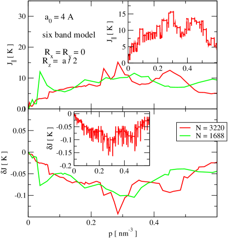
Figure 2: Effective exchange $J$ and anisotropy $\delta J$ for two Mn ions. We used the cut-off scheme (20) with $a_{0}=4\;\AA$, and a cut-off energy $E_{\rm cutoff}=3273\;{\rm K}$. The main parts show the obtained interaction for $L=23a$ and $L=29a$ at concentrations corresponding to “closed shells”, while the insets show the $L=29a$ results for all concentrations.

In Fig. 2 we show the obtained effective interaction as a function of the hole concentration $p$ for two different numbers of $k$-points ($N$) below the cut-off energy $E_{\rm cutoff}=3273{\rm K}$ for a Mn separation of $R=a/2\approx 2.8\AA$. For these calculations we used a dimensionless coupling, $j_{pd}\equiv{SJ_{pd}m\over a^{3}4\pi^{3}}=0.2$, with $S=5/2$ the Mn spin, $m$ the free electron mass, and $a=5.65\AA$ the lattice constant. This value of $j_{pd}$ roughly corresponds to the exchange coupling used in Ref. [Brey and Gómez-Santos, 2003]. The accuracy of the calculation can be inferred both from the difference between the $N=3220$ and $N=1688$ data, and from the size of the discrete jumps. It is around $10-20\%$ at best. Thus, one cannot give a quantitatively reliable estimation of the anisotropy from these numerical calculations. In this regard it is somewhat misleading that for a fixed number of holes the exchange energy behaves very nicely as a function of the angle of the two magnetic impurities,Brey and Gómez-Santos (2003) as demonstrated in Fig. 3. In fact, our experience with other local density of states calculations shows that one may need around $10^{6}$ k-points to achieve an accuracy of $\sim 1\%$, which seems to be beyond the scope of present-day numerics.foo (b)

It is therefore questionable how well these data can be trusted in regard to the estimation of the anisotropy energy. However, a qualitative assessment can be made. While anisotropy energies $\delta J$ are definitely smaller than the numerical errors of the total exchange energies, they still show a consistent pattern (see Fig. 2), suggesting that the order of magnitude of the anisotropy $\delta J/J_{||}$ is probably correctly given, even for these small values of $N$.

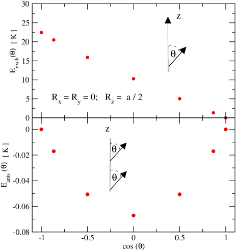
Figure 3: Spin orientation dependence of the ground state energy for a fixed number of holes corresponding to a hole concentration of $p=0.2{\rm nm}^{-3}$: (a) One of the spins is aligned along the $z$-axis, and the other is rotated in the $xz$ plane. (b) The spins are parallel and rotated in the $xz$ plane.

The anisotropy in Fig. 2 for a Mn separation of $R\approx 2.8\AA$ is much smaller than the one obtained within the spherical approximation. This somewhat surprising result can be understood as follows: for short Mn-Mn separations the exchange interaction is dominated by high energy electron-hole excitations. However, as shown in Fig. 4, the four band model ($\Delta_{SO}\to\infty$) provides a good approximation to the exact eigenstates only up to energies $E\sim 0.15-0.2{\rm eV}$, corresponding to hole concentrations up to $p\sim 0.3-0.4{\rm nm}^{-3}$. For these high-energy excitations it therefore fails and largely overestimates the strength of spin-orbit interaction.

On the other hand, for hole concentrations less than $p\sim 0.3\ {\rm nm}^{-3}$ the Fermi energy is in a range where the $\Delta_{SO}\to\infty$ approximation for the single particle states is appropriate. While for short Mn-Mn separations, electron-hole excitations at all energy scales contribute to the RKKY interaction, for larger values of $R$ the RKKY interaction is dominated by electron-hole excitations in the vicinity $\delta k\sim 1/R$ of the Fermi surface. We expect therefore that the anisotropy will increase for these concentrations with increasing Mn-Mn separation $R$.

These expectations are indeed supported by our numerical results shown in Fig. 5, where we find that the typical anisotropy, $\delta J/J_{||}$ increases with the Mn-Mn separation and becomes of the order of $\sim 20\%$ for the typical Mn-Mn separation $R\sim 10\AA$ at $x=0.05$ Mn content.

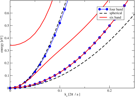
Figure 4: Comparison of the hole dispersion within the full six band model, the four band model, and the spherical approximation. The latter two are reasonable approximations for $E_{F}<0.15-0.2{\rm eV}$, which corresponds to a hole density of $p<0.25-0.4{\rm nm}^{-3}$.

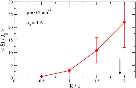
Figure 5: Average anisotropy for $0.2{\rm nm}^{-3}<p<0.3{\rm nm}^{-3}$. We used the same parameters as in Fig. 2. The anisotropy increases with distance and becomes of the size $\sim 20\%$ for $R=2a$, which is around the typical Mn-Mn distance for $x=5\%$, indicated by the arrow.

In Fig. 6 we show the exchange interaction and the anisotropy as a function of the separation of the two Mn ions for various hole concentrations. The exchange interaction increases monotonically as the hole concentration is increased, while the “interaction range” decreases due to the increase of the Fermi momentum. The maximum of the anisotropy term, on the other hand, decreases for larger hole concentrations, since then the Fermi energy moves into a range where spin-orbit coupling is of lesser importance. Depending on the specific value of hole concentration, the size of the anisotropy is in the range of $10-30\%$ for typical Mn separations.

Regarding the directional anisotropy (from the cubic symmetry of the lattice) mentioned in Ref. [Brey and Gómez-Santos, 2003] we remark that while spin anisotropy can induce a frustrated ground state and may thus also change the universality class of the ferromagnetic transition, directional anisotropy only increases the already existing disorder somewhat, and does not induce any frustration. As a consequence, it does not change the magnetic properties of the system, and plays an unimportant role in an already disordered ferromagnet.

In the calculations above we neglected disordered Coulomb scattering of the valence holes on static impurities (As antisites and Mn core charges etc.). This type of disorder destroys the coherent propagation of the electrons and therefore reduces the value of both $J_{||}$ and $\delta J$ for separations larger than the electronic mean free path $\ell$. For the metallic samples $\ell$ is of the order of the typical Mn-Mn separation, and therefore we expect that the suppression is not dramatic. While it is not clear how much the ratio $\delta J/J_{||}$ is reduced by static disorder, it is likely that random anisotropy effects are important for the disordered samples too.

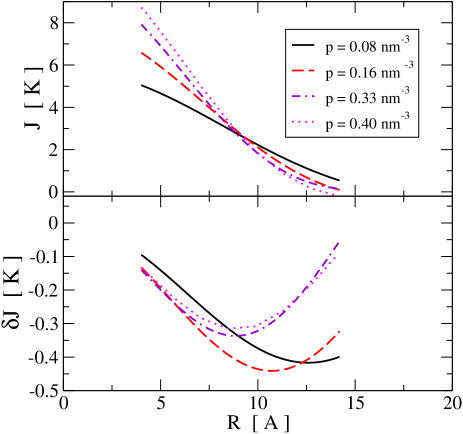
Figure 6: Position- and hole concentration-dependence of the exchange and anisotropy of the RKKY interaction within the six band model.

IV Monte Carlo Study

Having obtained the effective kernels, in this section we report the results of classical Monte Carlo (MC) calculations in the spin degrees of freedom used to study the implications of anisotropy on the magnetic properties of ${\rm Ga}_{1-x}{\rm Mn}_{x}{\rm As}$. Similar Monte Carlo studies of GaMnAs have also been carried out on other modelsSchliemann et al. (2001); Kennett et al. (2002); Brey and Gómez-Santos (2003).

The properties of the obtained ferromagnetic state are expected to depend on correlations between the positions of Mn spins. As we mentioned in the introduction, it is presently unknown from the available experimental data to what extent the substitutional, magnetically active, Mn positions are correlated. It is therefore worthwhile to investigate theoretically the trends in magnetic properties as a function of increasing correlations in the Mn ion positions. We applied the spin-spin interaction kernels computed in the first part of this paper to monitor how the magnetic properties such as the saturation magnetization, the Curie temperature, the shape of the magnetization curves and the spin distributions change as Mn positional correlations are gradually built in via the procedure described below.

To simulate positional correlations and to control disorder we first generate a completely random Mn distribution within the Ga sublattice of an $L\times L\times L$ cube of ${\rm Ga}_{1-x}{\rm Mn}_{x}{\rm As}$, and then relax the Mn ions through a standard $T=0$ Monte Carlo procedure with nearest and next nearest neighbor hopping, assuming a screened Coulomb interaction between the Mn ions. It is extremely important to use periodic boundary conditions in the course of this relaxation procedure, otherwise the Mn ions accumulate on the surface of the cube.

The typical evolution of the average nearest neighbor distance with MC time, $t_{MC}$, is shown in Fig. 7 for two different sample sizes and $x=0.05$. Correlations are formed within a MC time span of $t_{MC}\sim 5$. A careful investigation of these correlations for dilute samples with $x\sim 0.01\;-\;0.02$ shows that the Mn ions tend to form a somewhat distorted BCC lattice with point defects. In the following, we shall use this Monte Carlo time as a parameter to control the amount of positional disorder.

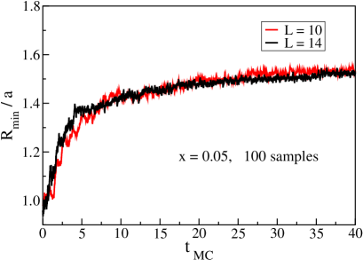
Figure 7: Average nearest neighbor Mn distance vs. Monte Carlo time for $L=12a$ and $L=17a$.

In all simulations to be described below the Mn spins were replaced by their classical angular variables ${\bf S\to}S\;{\bf\Omega}$, which is expected to be a reasonable approximation for $S=5/2$. To take account of the finite mean free path $l\approx 7$Å of the valence holesOhno et al. (1992); D. J. Priour et al. (2004), we used an exponential cutoff for the RKKY interaction: $K_{\rm para/perp}({\bf R})\to K_{\rm para/perp}({\bf R})e^{-R/l}$. We also introduced a hard cutoff for the effective interaction, $l_{\rm hard}=2r_{\rm Mn}$, where $r_{\rm Mn}$ is related to the Mn concentration, $n_{\rm Mn}=[4\pi\;r_{\rm Mn}^{3}/3]^{-1}$. This hard cut-off has been defined to take into account that the RKKY approximation does not make any sense beyond the first “shell” of neighbors, since Mn ions are very strong potential scatterers.

IV.1 Monte Carlo results within the spherical approximation

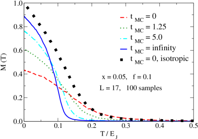
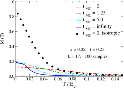
Figure 8: Magnetization vs. temperature for hole fractions $f=0.10$ (top) and $f=0.25$ (bottom) as a function of Monte Carlo time. Note that for $f=0.1$ the isotropic kernel results in nearly full polarization even for the completely disordered sample demonstrating the the reduction of the magnetization is dominantly due to anisotropy effects.

Within the spherical approximation, the results depend almost exclusively on the hole fraction $f$ and do not depend too much on the specific value of the Mn concentration $x$. This is because the effective kernel depends on the Mn-Mn distance through $y=k_{F,h}R$. The typical values of $y$ depend on $f$. However, lattice-specific effects play a less important role in the dilute limit, where characteristic distances are typically much larger than the lattice constant.

In Fig. 8 we show the temperature-dependence of the magnetization $M\equiv|\langle\Omega_{i}\rangle|$, for different amounts of disorder, as a function of temperature for two different hole fractions, $f=0.1$ and $f=0.25$. A spontaneous magnetization develops at low temperatures in both cases. For small Monte Carlo times (large disorder) the transition between the paramagnetic and magnetic phases takes place rather smoothly, and then the magnetization increases approximately linearly with decreasing temperature, qualitatively similar to many experiments.Esch et al. (1997); Potashnik et al. (2001) The Curie temperature (estimated by where the curves would intersect the temperature axis if the high temperature tails are ignored) decreases with decreasing disorder, i.e., disorder tends to enhance the transition temperature.Berciu and Bhatt (2001); Bhatt and Wan (1999); Berciu and Bhatt (2004) While the $M(T)$ curves of the unrelaxed samples do not quite look like usual mean-field magnetization curves, they become more and more mean-field-like upon relaxing the Mn impurity positions. All these properties are characteristic of strongly disordered magnets and have been reported earlier.Berciu and Bhatt (2001)

For both hole fractions we find that the magnetization tends to a value at $T=0$ that is smaller than that of a fully polarized ferromagnet. This effect is mostly due to anisotropy induced frustration: We recover the fully polarized state when we substitute the kernel with its angle averaged value.

Correlations between the Mn sites decrease frustration effects and tend to increase this remnant magnetization, and for $f=0.1$ the fully relaxed system recovers $90\%$ of the magnetization (see Fig. 10). The corresponding evolution of the distribution of the ground state spin orientations is shown in Fig. 9. The angle $\theta$ in Fig. 9 denotes the angle with respect to the direction of the ground state magnetization vector, ${\bf n}:{\rm cos}\theta_{i}={\bf\Omega_{i}\cdot n}$. When all spins are aligned, $P({\rm cos}\theta)=\delta(1-{\rm cos}\theta)$, and the more ordered the positions of the Mn ions, the more peaked the distribution becomes around $\cos\theta=1$.

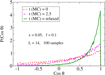
Figure 9: Ground state spin distribution for $f=0.10$. The angle $\theta$ is measured with respect to the ground state magnetization.

The simulations with $f=0.25$ show a much stronger reduction of the zero temperature magnetization relative to the case of $f=0.10$, even for the relaxed samples. Furthermore, for a fixed disorder the Curie temperature is reduced by about $20\;-\;40\%$ for $f=0.25$ with respect to that of $f=0.1$, even if we take into account the factor of $\sim 3$ increase in the energy scale $E_{J}$. In view of the results of the following section, we believe that these results are artifacts of the spherical approximation: As we emphasized earlier, within the spherical approximation oscillations appear in the interaction kernel, which show rather specific features around $y=k_{F,h}R\sim 2$, which is just the typical value of $y$ for $f=0.25$. While for $f=0.10$ the parallel component of the kernel is ferromagnetic for typical Mn-Mn separations, for $f=0.25$ it becomes antiferromagnetic. Therefore it is likely that for $f=0.25$ both the anisotropy and the antiferromagnetic part of the RKKY coupling play an important role.Zhou et al. (2004)

The main effects due to correlations between the Mn impurities are summarized in Fig. 10, where we show the $T=0$ magnetization for $L/a=17$ and the $L=\infty$ extrapolated value of $T_{C}$ as a function of Monte Carlo time. This latter has been obtained by measuring the maximum of the susceptibility for various system sizes and then extrapolating to $L=\infty$ by using the critical exponents for the Heisenberg model known from $\epsilon$ expansion.Guillou and Zinn-Justin (1980) Both quantities change monotonically with disorder, with a time scale similar to the one with which the disorder changes (see Fig. 7).

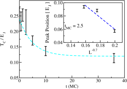
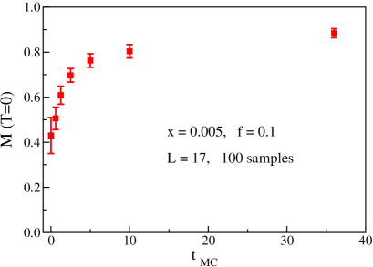
Figure 10: Top panel: the $L=\infty$ extrapolated Curie temperature as a function of Monte Carlo time. The dashed curves are a guide to the eye; Inset to top panel: The scaling of the peak in susceptibility with system size $L$, for $t_{MC}=2.5$;Bottom panel: $M(T=0)$ for $f=0.10$ and $L=17a$.

IV.2 Monte Carlo results within the six band model

In this subsection we study the magnetic properties of Ga_1-xMn_xAs using the effective interaction kernel computed within the six band model. In this case the interaction kernel depends on the specific direction of the two Mn ions, and, in principle, one should compute it for all possible positions of the two Mn ions, as the effective interaction is, in general, a rather complicated tensor. This is next to impossible, and besides, we do not expect to obtain quantitatively correct results from it anyway, since in these calculations we neglect the polarization of the holes in the ferromagnetic state, the strong potential scattering off the Mn cores, and the effects of various defects in Ga_1-xMn_xAs.

Instead, to obtain a qualitative picture, we will pursue the following strategy: By tetragonal symmetry, the effective Mn spin-spin interaction kernel reduces to the simple form Eq. (11) provided that the two Mn ions are aligned along the $x$, $y$, or $z$ direction. We will therefore use the effective interaction Eq. (11), but we will substitute the kernels in this expression by the ones we computed in Section III. In this way we obtain a qualitatively correct description of the interaction between the Mn spins in Ga_1-xMn_xAs, which captures approximately the spin-orbit coupling induced anisotropy effects.

In this case the structure of the $M(T)$ curves depends not only on the hole fraction $f$, but also on the Mn concentration. In fact, our results show that for the active Mn concentration range $0.03<x<0.05$, $T_{C}$ is very sensitive to the Mn concentration $x$, but exhibits a much weaker dependence on the hole fraction. This originates from the specific property of the interaction kernel shown in Fig. 6. As we showed in the previous section, the role of spin-orbit coupling induced anisotropy is also more pronounced for larger Mn-Mn separations, i.e., smaller Mn concentrations.

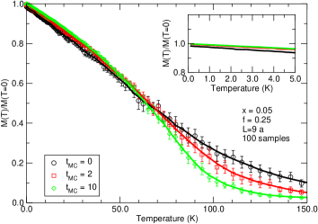
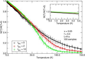
Figure 11: Temperature-dependence of the magnetization for a sample of linear size $L=9\;a$ with active Mn concentration $x=0.05$, hole fractions $f=0.25$ and $f=0.4$ as a function of Monte Carlo relaxation time. The insets show the low temperature saturation of the magnetization.

Typical magnetization curves are shown in Figs. 11 and 12 for $x=0.05$ and $x=0.03$. For $x=0.05$ the ground state is always almost fully polarized, even for the fully disordered, unrelaxed sample, only $T_{C}$ is gradually suppressed upon relaxing the impurity positions. For $x=0.03$, however, a slight non-collinearity appears for the fully disordered sample, corresponding to a $4\%$ suppression of the total magnetization and a typical angle between the ground state of the sample and an individual spin of the order of $\theta\sim 16$ degrees. This non-collinearity disappears once we introduce correlations between the Mn sites. These results clearly show that for larger Mn concentrations the spherical approximation badly fails and a more complete six band model must be used.

We also find that for even smaller concentrations, $x<0.03$, the spin-orbit coupling induced disorder plays a more important role, and the obtained ground state is non-collinear, similar to the one obtained within the spherical approximation. These results indicate that non-collinear states may appear for smaller Mn concentrations. This small concentration regime is, however, definitely out of reach for an RKKY approach: At these small concentration disorder also plays an important role and most likely an impurity band description of the material is necessaryFiete et al. (2003); Berciu and Bhatt (2001, 2004).

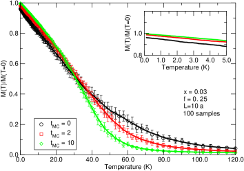
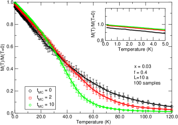
Figure 12: Temperature-dependence of the magnetization for a sample of linear size $L=10\;a$ with active Mn concentration $x=0.03$, hole fractions $f=0.25$ and $f=0.4$ as a function of Monte Carlo relaxation time. The insets show the low temperature saturation of the magnetization.

V Conclusions

In this paper we continued the route of Ref. [Zaránd and Jankó, 2002] to build effective spin models for metallic ${\rm Ga}_{1-x}{\rm Mn}_{x}{\rm As}$. We constructed interactions between the Mn spins mediated via indirect exchange by using two different valence band models. First we computed the effective interaction within the spherical approximation, where the calculations can be performed analytically, and then we studied the effective interaction numerically using the more complete six band model, also studied in Ref. [Brey and Gómez-Santos, 2003].

We find, in agreement with Ref. [Brey and Gómez-Santos, 2003], that the spherical approximation badly fails for short Mn separations where it overestimates the strength of the spin-orbit coupling induced anisotropy by more than one order of magnitude. However, we find using the six band model, that the strength of the spin-orbit coupling induced anisotropy increases with Mn-Mn distance, and becomes of the order of $\sim 20\%$, qualitatively (but not quantitatively) agreeing with the results obtained using the spherical approximation and also in rough agreement with the experimentally observed FMR linewidth.Rappoport et al. (2004); Liu et al. (2003) This implies that the frustration effects discussed in Ref. [Zaránd and Jankó, 2002] are probably more pronounced for small Mn concentrations.

We carried out classical Monte Carlo simulations to study the implications of the computed effective interactions. Within the spherical approximation, we always find a generically non-collinear state due to orientational frustration (random anisotropy). It has been speculated earlier that this state may be a ferromagnetic state of spin glass nature.Zaránd and Jankó (2002) However, our studies of hysteresis indicate that this random anisotropy results in a conventional, though non-collinear and disordered ferromagnetic state. This result seems to be supported by the fact that random anisotropy is presumably irrelevant at the Heisenberg fixed point,Chayes et al. (1986) and therefore does not change the critical scaling of a Heisenberg magnet.

The strongly non-collinear states found within the spherical model are partly an artifact of the spherical approximation, which is only valid at sufficiently small hole concentrations. Using the effective interaction obtained within the six band model of the valence holes, we find that the anisotropy effects are too weak to induce a strongly non-collinear state for (active) Mn concentrations as large as $x=0.05$. However, anisotropy becomes more important for lower concentrations, where it may induce a frustrated and non-collinear state.Fiete et al. (2003) In particular, for $x=0.03$ we find that the ground state of the fully disordered sample is not fully collinear, and individual spins deviate from the ferromagnetic orientation of the sample by about $\sim 16$ degrees. This tendency is expected to be even more pronounced for lower Mn concentrations where we expect a non-collinear ferromagnetic state.Fiete et al. (2003) Indeed, for Mn concentrations in the range $x=0.015-0.02$ we find a non-collinear state similar to the one obtained in the spherical approximation, though this concentration range may already be well out of the range of the metallic approximation used in this paper, and the impurity band approach of Refs. [Fiete et al., 2003; Berciu and Bhatt, 2001, 2004] may be more appropriate in this limit. Experimental evidence also supports the presence of a non-collinear state in the regime of small Mn concentrations.Potashnik et al. (2003)

Let us emphasize again, that the Mn concentrations above denote the concentration of active substitutional Mn ions, which can be substantially smaller than the nominal Mn concentration of the samples.Yu et al. (2002a); Edmonds et al. (2004) In particular, it is known that a substantial amount of the dopant Mn ions go to interstitial sites in course of the out-of equilibrium growth process,Yu et al. (2002a); Edmonds et al. (2004) and these interstitial Mn ions are also believed to bind to the substitutional Mn ions and “neutralize” them from the point of view of ferromagnetism.Bergqvist et al. (2003) In this way, it is quite possible that an unannealed sample with a nominal Mn concentration of $x_{\rm nom}\sim 0.05$ has an active Mn concentration of only around $x=0.01-0.03$ and have a non-collinear ground state. It is, on the other hand quite likely that annealed samples and samples with higher Mn concentrations form a ferromagnetic state where the Mn spins are almost perfectly collinear.

As first pointed out in Ref. [Zaránd and Jankó, 2002], the observed saturation magnetization of ${\rm Ga}_{1-x}{\rm Mn}_{x}{\rm As}$ is much less even in annealed samples than expected based on the nominal Mn concentration of the samples. The orientational frustration discussed in this paper provides a possible mechanism to explain the missing magnetization in unannealed and “underdoped” samples, where one can substantially increase the saturation value of the magnetization, $M(T=0)$ with a relatively small magnetic field compared to $T_{C}$, $H<1\;{\rm T}$.Potashnik et al. (2003) Other mechanisms have also been proposed: The main mechanism that reduces the magnetization of annealed samples seems to be provided by the presence of interstitial Mn ions, which - as mentioned earlier - “neutralize” substitutional Mn impurities.Bergqvist et al. (2003) It has also been proposed that As antisite defects can induce a non-collinear state,Korzhavyi et al. (2002) and an intrinsic non-collinearity has been proposed also in Ref. [Schliemann, 2003; Schliemann and MacDonald, 2002]. Finally, quantum fluctuations due to the antiferromagnetic coupling between the Mn spins and the valence holes have been also proposed recently.Mac It is probably a combination of all these effects that is finally responsible for the missing magnetization of ${\rm Ga}_{1-x}{\rm Mn}_{x}{\rm As}$.

Finally, we comment on the approximations made in this paper. Throughout, we followed a common practice in the literature,Tim (a) and neglected the potential scattering off the Mn ions. This approximation is expected to produce qualitatively reliable results in the metallic limit considered and we believe that all the trends reported here are robust. We also neglected the polarization of the valence holes induced by the ferromagnetically alligned Mn spins, which may be important at low temperatures. In summary, we believe the answers to the questions of how anisotropic the Mn spin-spin interactions are in metallic GaMnAs and how anisotropy interplays with Mn positional correlations to affect important magnetic properties are now on more solid ground, though further studies are needed to understand frustration effects in the regime $x<0.03$.

NOTE: While preparing this work for publication, a preprint appearedTim (b) where the authors arrive at rather similar conclusions using a very different, tight binding approach.

Appendix A Calculation of RKKY Kernel

In this appendix, we derive explicit expressions for the kernels $K_{\rm par}(R)$ and $K_{\rm perp}(R)$ appearing in Eq. (9). By spherical symmetry, we can assume that the two Mn impurities are alligned along the $z$ axis. In this case, the kernel $K^{\alpha\beta}$ becomes diagonal, $K^{\alpha\beta}=K^{\alpha}\delta_{\alpha\beta}$, and can be written by converting the sums in Eq. (LABEL:eq:RKKY_sum) to integrals and assuming a parabolic dispersion for the light and heavy hole bands as

$$K^{\alpha\alpha}({\bf R})=2G^{2}\sum_{\mu\mu^{\prime}}\int_{0}^{k_{F,\mu}}{k^{2}dk\over 2\pi^{2}}\int_{k^{\prime}_{F,\mu}}^{\infty}{k^{\prime 2}dk^{\prime}\over 2\pi^{2}}{1\over{k^{\prime 2}\over 2m_{\mu^{\prime}}}-{k^{2}\over 2m_{\mu}}}\langle|J^{\alpha}_{\mu\mu^{\prime}}(\theta,\theta^{\prime},\phi,\phi^{\prime})|^{2}\,2\,{\rm cos}(kR{\rm cos}(\theta)-k^{\prime}R{\rm cos}(\theta^{\prime}))\rangle_{\theta,\theta^{\prime},\phi,\phi^{\prime}}\;.$$ (21)

Here we have taken the angles $\theta$ and $\phi$ ($\theta^{\prime}$ and $\phi^{\prime}$) parametrize the directions $\hat{\bf k}=(\sin\theta\cos\phi,\;\sin\theta\sin\phi,\;\cos\theta)$ and $\hat{\bf k^{\prime}}$, and the brackets denote the angular average over the angles $\theta,\theta^{\prime},\phi$ and $\phi^{\prime}$. Making the substitutions $k\to\sqrt{2m_{\mu}\epsilon_{F}}k$ and $k^{\prime}\to\sqrt{2m_{\mu^{\prime}}\epsilon_{F}}q$ yields the expression

$$K^{\alpha}({\bf R})=8\,\epsilon_{F}\sum_{\mu,\mu^{\prime}}g_{\mu}g_{\mu^{\prime}}\int_{0}^{1}dk\int_{1}^{\infty}dq{q^{2}k^{2}\over q^{2}-k^{2}}$$

$$\times I^{\alpha}_{\mu\mu^{\prime}}(k_{F,\mu}kR,k_{F,\mu^{\prime}}qR)\;,$$

(22)

where

$$I^{\alpha}_{\mu\mu^{\prime}}(k_{F,\mu}kR,k_{F,\mu^{\prime}}qR) = \langle|J^{\alpha}_{\mu\mu^{\prime}}(\theta,\theta^{\prime},\phi,\phi^{\prime})|^{2}\,$$

$$\times 2\,{\rm cos}(k_{F,\mu}kR{\rm cos}(\theta) - k_{F,\mu^{\prime}}qR{\rm cos}(\theta^{\prime}))\rangle_{\theta,\theta^{\prime},\phi,\phi^{\prime}}\;,$$

and we introduced the dimensionless couplings, $g_{\mu}=G\varrho_{\mu}=G{m_{\mu}^{3/2}\over\sqrt{2}\pi^{2}}\epsilon_{F}^{1/2}$.

To compute $K^{\alpha\alpha}({\bf R})$ we first evaluate $I^{\alpha}_{\mu\mu^{\prime}}(k_{F,\mu}kR,k_{F,\mu^{\prime}}qR)$ by performing the angular integrals. Since $I^{\alpha}_{\mu\mu^{\prime}}(k_{F,\mu}kR,k_{F,\mu^{\prime}}qR)$ only depends on $k$ and $q$ through the combinations $k_{F,\mu}kR$ and $k_{F,\mu^{\prime}}qR$, it is worth defining the heavy hole contributions to it as:

$$I^{\alpha}_{hh}\equiv I^{\alpha}_{\frac{3}{2},\frac{3}{2}}+I^{\alpha}_{\frac{3}{2},-\frac{3}{2}}+I^{\alpha}_{-\frac{3}{2},\frac{3}{2}}+I^{\alpha}_{-\frac{3}{2},-\frac{3}{2}}\;.$$ (24)

The contributions $I^{\alpha}_{hl}$, $I^{\alpha}_{lh}$, and $I^{\alpha}_{ll}$, and the corresponding contributions to the kernel, $K^{\alpha}_{hh}$, $K^{\alpha}_{lh}$, $K^{\alpha}_{hl}$, $K^{\alpha}_{ll}$, can be defined in an analogous way.

We demonstrate the procedure of computing $K^{\alpha}$ by the example of the heavy hole contribution to $K^{z}_{hh}$. It is straightforward to evaluate the angular integrals, and for $I^{z}_{hh}$ one obtains the following expression:

$$I^{z}_{hh}(rk,rq)={9\over 10}{{\rm sin}(kr)\over kr}{{\rm sin}(qr)\over qr}$$

$$+{45\over 2}\Biggl{(}{{\rm cos}(kr)\over k^{2}r^{2}}-{{\rm sin}(kr)\over k^{3}r^{3}}+{3\over 5}{{\rm sin}(kr)\over kr}\Biggr{)}$$

$$\times\Biggl{(}{{\rm cos}(qr)\over q^{2}r^{2}}-{{\rm sin}(qr)\over q^{3}r^{3}}+{3\over 5}{{\rm sin}(qr)\over qr}\Biggr{)}\;,$$ (25)

which can be rewritten as

$$I^{z}_{hh}(rk,rq)={9\over 10}\frac{F(k)F(q)}{kq}+{45\over 2}\frac{G(k)G(q)}{kq}\;,$$ (26)

where $F$ and $G$ have the obvious definitions. The heavy hole contribution to $K^{z}(R)$ thus reads

$$K^{z}_{h,h}({\bf R})=8\,\epsilon_{F}g_{h}^{2}\int_{0}^{1}\!\!\!\!dk\int_{1}^{\infty}\!\!\!\!\!\!dq {1\over q^{2}-k^{2}}\Biggl{[}{9\over 10}kqF(k)F(q)$$ (27)

$$+{45\over 2}kqG(k)G(q)\Biggr{]}\;.$$

As shown in Appendix B, for $F$ and $G$ of the form that appear in Eq. (22) the integrals over $q$ in Eq. (27) can be carried out to give

$$\int_{0}^{1} dk \int_{1}^{\infty}dq{qk\over q^{2}-k^{2}}F(k)F(q)=$$ (28)

$$= {\pi\over 2}i\int_{0}^{1}dkk\Biggl{[}F^{+}(k)^{2}-F^{-}(k)^{2}$$

$$+ F(k){\rm lim_{q\to 0}}\left\{{2q^{2}\over q^{2}-k^{2}}F^{+}(q)\right\}\Biggr{]}\;,$$

where $F^{+}$ and $F^{-}$ denote the parts of the function $F=F^{+}+F^{-}$ which are analytical on the upper and lower half-planes, respectively. Applying this formula, we obtain upon making the substitution $a=k_{F,h}R$ and $b=k_{F,l}R$

$$K^{zz}_{h,h}({\bf R})=4\pi\,\epsilon_{F}g_{h}^{2}\int_{0}^{1}dk\Biggl{[}\frac{9}{20}\frac{k\,{\rm sin}(2ka)}{a^{2}}$$

$$+\frac{45}{2}\Biggl{(}\frac{{\rm cos}(ka)}{a^{5}k^{2}}+\frac{3{\rm cos}(2ka)}{5a^{3}}-\frac{3{\rm cos}(2ka)}{a^{5}k^{2}}-\frac{{\rm sin}(ka)}{a^{6}k^{3}}$$

$$+\frac{3{\rm sin}(ka)}{5a^{4}k}+\frac{{\rm sin}(2ka)}{2a^{6}k^{3}}-\frac{11{\rm sin}(2ka)}{10a^{4}k}+\frac{9{\rm sin}(2ka)}{50a^{2}}\Biggr{)}\Biggr{]}$$

$$\equiv 4\pi\,\epsilon_{F}g_{h}^{2}C_{\rm para}^{\rm heavy}(a)\;.\;\;\;\;\;\;\;\;\;\;\;\;\;\;$$ (29)

It is also possible to evalute the integral (29), but the resulting formula is very long, and for practical purposes it is simpler to evaluate Eq. (29) numerically.

The remaining parts of the kernel can be evaluated in a similar way, and are given below. By symmetry, $K^{x}=K^{y}$ for this arrangement, and therefore only the $x$-component is displayed. The spatial dependence of the various parts of the kernel is shown in Fig. 1.

$$K^{xx}_{h,h}({\bf R})=4\pi\,\epsilon_{F}g_{h}^{2}\int_{0}^{1}dk\frac{9}{2}\Biggl{[}-\frac{{\rm cos}(ka)}{a^{5}k^{2}}-\frac{{\rm cos}(2ka)}{a^{3}}+\frac{{\rm cos}(2ka)}{a^{5}k^{2}}+\frac{{\rm sin}(ka)}{a^{6}k^{3}}-\frac{{\rm sin}(ka)}{a^{4}k}-\frac{{\rm sin}(2ka)}{2a^{6}k^{3}}+\frac{3{\rm sin}(2ka)}{2a^{4}k}\Biggr{]}\;.$$

$$K^{zz}_{h,l}({\bf R}) + K^{zz}_{l,h}({\bf R})=4\pi\,\epsilon_{F}g_{h}g_{l}\int_{0}^{1}dk\Biggl{[}\frac{3}{2}\Biggl{(}-\frac{{\rm cos}(ka){\rm cos}(kb)}{a^{2}b}+\frac{{\rm cos}(ka){\rm sin}(ka)}{a^{6}k^{3}}+\frac{{\rm cos}(ka){\rm sin}(ka)}{a^{4}k}+\frac{{\rm cos}(kb){\rm sin}(ka)}{a^{3}bk}$$ (30)

$$- \frac{{\rm sin}(2ka)}{2a^{6}k^{3}}-\frac{{\rm sin}(2ka)}{2a^{4}k}-\frac{{\rm sin}(kb)}{a^{3}bk}+\frac{{\rm cos}(ka){\rm sin}(kb)}{a^{3}bk}+\frac{{\rm sin}(ka){\rm sin}(kb)}{a^{2}b}\Biggr{)}$$

$$+ \frac{45}{2}\Biggl{(}-\frac{{\rm cos}(ka)}{a^{2}b^{3}k^{2}}-\frac{{\rm cos}(kb)}{a^{3}b^{2}k^{2}}+\frac{{\rm cos}(ka){\rm cos}(kb)}{a^{2}b^{3}k^{2}}+\frac{{\rm cos}(ka){\rm cos}(kb)}{a^{3}b^{2}k^{2}}+\frac{{\rm sin}(ka)}{a^{3}b^{3}k^{3}}-\frac{{\rm cos}(kb){\rm sin}(ka)}{a^{3}b^{3}k^{3}}$$

$$+ \frac{{\rm cos}(kb){\rm sin}(ka)}{a^{2}b^{2}k}+\frac{{\rm sin}(kb)}{a^{3}b^{3}k^{3}}-\frac{{\rm cos}(ka){\rm sin}(kb)}{a^{3}b^{3}k^{3}}+\frac{{\rm cos}(ka){\rm sin}(kb)}{a^{2}b^{2}k}-\frac{{\rm sin}(ka){\rm sin}(kb)}{a^{2}b^{3}k^{2}}-\frac{{\rm sin}(ka){\rm sin}(kb)}{a^{3}b^{2}k^{2}}\Biggr{)}$$

$$+ \frac{27}{2}\Biggl{(}-\frac{{\rm cos}(ka){\rm cos}(kb)}{ab^{2}}-\frac{{\rm sin}(ka)}{ab^{3}k}+\frac{{\rm cos}(kb){\rm sin}(ka)}{ab^{3}k}+\frac{{\rm cos}(ka){\rm sin}(kb)}{ab^{3}k}+\frac{{\rm cos}(kb){\rm sin}(kb)}{b^{6}k^{3}}$$

$$+ \frac{{\rm cos}(kb){\rm sin}(kb)}{b^{4}k}+\frac{{\rm sin}(ka){\rm sin}(kb)}{ab^{2}}-\frac{{\rm sin}(2kb)}{2b^{6}k^{3}}-\frac{{\rm sin}(2kb)}{2b^{4}k}\Biggr{)}\Biggr{]}\;.$$

$$K^{xx}_{h,l}({\bf R}) + K^{xx}_{l,h}({\bf R})=4\pi\,\epsilon_{F}g_{h}g_{l}\int_{0}^{1}dk\Biggl{[}\frac{3}{2}\Biggl{(}-\frac{{\rm cos}(ka){\rm cos}(kb)}{a^{2}b}+\frac{{\rm cos}(ka){\rm sin}(ka)}{a^{6}k^{3}}+\frac{{\rm cos}(ka){\rm sin}(ka)}{a^{4}k}+\frac{{\rm cos}(kb){\rm sin}(ka)}{a^{3}bk}$$ (31)

$$-\frac{{\rm sin}(2ka)}{2a^{6}k^{3}}-\frac{{\rm sin}(2ka)}{2a^{4}k}-\frac{{\rm sin}(kb)}{a^{3}bk}+\frac{{\rm cos}(ka){\rm sin}(kb)}{a^{3}bk}+\frac{{\rm sin}(ka){\rm sin}(kb)}{a^{2}b}\Biggr{)}$$

$$+ \frac{9}{2}\Biggl{(}\frac{{\rm cos}(ka)}{a^{2}b^{3}k^{2}}+\frac{{\rm cos}(kb)}{a^{3}b^{2}k^{2}}+\frac{{\rm cos}(ka){\rm cos}(kb)}{ab^{2}}-\frac{{\rm cos}(ka){\rm cos}(kb)}{a^{2}b^{3}k^{2}}-\frac{{\rm cos}(ka){\rm cos}(kb)}{a^{3}b^{2}k^{2}}-\frac{{\rm sin}(ka)}{a^{3}b^{3}k^{3}}+\frac{{\rm sin}(ka)}{ab^{3}k}$$

$$+ \frac{{\rm cos}(kb){\rm sin}(ka)}{a^{3}b^{3}k^{3}}-\frac{{\rm cos}(kb){\rm sin}(ka)}{ab^{3}k}-\frac{{\rm cos}(kb){\rm sin}(ka)}{a^{2}b^{2}k}-\frac{{\rm sin}(kb)}{a^{3}b^{3}k^{3}}+\frac{{\rm cos}(ka){\rm sin}(kb)}{a^{3}b^{3}k^{3}}-\frac{{\rm cos}(ka){\rm sin}(kb)}{ab^{3}k}$$

$$- \frac{{\rm cos}(ka){\rm sin}(kb)}{a^{2}b^{2}k}-\frac{{\rm cos}(kb){\rm sin}(kb)}{b^{6}k^{3}}-\frac{{\rm cos}(kb){\rm sin}(kb)}{b^{4}k}-\frac{{\rm sin}(ka){\rm sin}(kb)}{ab^{2}}+\frac{{\rm sin}(ka){\rm sin}(kb)}{a^{2}b^{3}k^{2}}+\frac{{\rm sin}(ka){\rm sin}(kb)}{a^{3}b^{2}k^{2}}$$

$$+ \frac{{\rm sin}(2kb)}{2b^{6}k^{3}}+\frac{{\rm sin}(2kb)}{2b^{4}k}\Biggr{)}+3\Biggl{(}\frac{k\,{\rm cos}(ka){\rm sin}(ka)}{a^{2}}+\frac{k\,{\rm cos}(kb){\rm sin}(ka)}{ab}-\frac{k\,{\rm sin}(2ka)}{2a^{2}}+\frac{k\,{\rm cos}(ka){\rm sin}(kb)}{ab}$$

$$+ \frac{k\,{\rm cos}(kb){\rm sin}(kb)}{b^{2}}-\frac{k\,{\rm sin}(2kb)}{2b^{2}}\Biggr{)}\Biggr{]}\;.$$

$$K^{zz}_{l,l}({\bf R}) = 4\pi\,\epsilon_{F}g_{l}^{2}\int_{0}^{1}dk\Biggl{[}\frac{9{\rm sin}(2kb)}{20a^{2}}+\frac{45}{2}\Biggl{(}\frac{{\rm cos}(kb)}{a^{5}k^{2}}+\frac{{\rm cos}(2kb)}{15b^{3}}-\frac{{\rm cos}(2kb)}{b^{5}k^{2}}-\frac{{\rm sin}(kb)}{b^{6}k^{3}}+\frac{{\rm sin}(kb)}{15b^{4}k}$$ (32)

$$+ \frac{{\rm sin}(2kb)}{2b^{6}k^{3}}-\frac{17{\rm sin}(2kb)}{30b^{4}k}+\frac{k\,{\rm sin}(2kb)}{450b^{2}}\Biggr{)}\Biggr{]}\;.$$

$$K^{xx}_{l,l}({\bf R}) = 4\pi\,\epsilon_{F}g_{l}^{2}\int_{0}^{1}dk\frac{9}{2}\Biggl{[}-\frac{{\rm cos}(kb)}{b^{5}k^{2}}+\frac{{\rm cos}(2kb)}{3b^{3}}+\frac{{\rm cos}(2kb)}{b^{5}k^{2}}+\frac{{\rm sin}(kb)}{b^{6}k^{3}}+\frac{{\rm sin}(kb)}{3b^{4}k}-\frac{{\rm sin}(2kb)}{2b^{6}k^{3}}$$ (33)

$$+\frac{{\rm sin}(2kb)}{6b^{4}k}+\frac{4k\,{\rm sin}(2kb)}{9b^{2}}\Biggr{]}\;.$$

Appendix B Evaluation of Singular RKKY Integrals for Spin 3/2 Particles

In this appendix we establish the identity Eq. (28). First we note that the functions $F(k)$ that appear in the evaluation of the RKKY kernel, Eq. (22), have two important properties that we will use in course of the derivation: (i) they are odd, $F(-k)=-F(k)$ and (ii) $F$ is regular at the origin.

First let us prove that

$$I={\rm lim}_{\delta\to 0}\int_{-1+i\delta}^{1+i\delta}dz\int_{-1}^{1}dq{qz\over q^{2}-z^{2}}F(z)F(q)=0\;,$$ (34)

where $\delta$ is a positive infinitesimal quantity. Decomposing the integrand ${q\over q^{2}-z^{2}}=\frac{1}{2}\left(\frac{1}{q-z}+\frac{1}{q+z}\right)$, introducing the variable $x=z-i\delta$ $I$, and using the identity $\frac{1}{x\pm i\delta}={\cal P}\frac{1}{x}\mp i\pi\delta(x)$ we rewrite $I$ as

$$I = \int_{-1}^{1}dx\int_{-1}^{1}dq\Biggl{[}P{q\over q^{2}-x^{2}}$$ (35)

$$+ i\frac{\pi}{2}\delta(q-x)-i\frac{\pi}{2}\delta(q+x)\Biggr{]}xF(x)F(q)\;,$$

where $P$ denotes the principal part of the integral. The principal value integral over the first term is zero by symmetry, and the integral over the last two terms terms simply evaluates to $i\frac{\pi}{2}(qF(q)F(q)-(-q)F(-q)F(q))=0$, since $F(-q)=-F(q)$.

We now return to the formula, Eq. (28). Using Eq. (34) and the fact that the integrand in Eq. (28) is even in both $k$ and $q$, we can extend the region of integration to obtain

$$\int_{0}^{1}dk\int_{1}^{\infty}dq{qk\over q^{2}-k^{2}}F(k)F(q)=$$

$${\rm lim}_{\delta\to 0}\frac{1}{8}\int_{C}dz\int_{-\infty}^{\infty}dq\;z\;kF(z)\left(\frac{1}{q-z}+\frac{1}{q+z}\right)F(q)\;,$$

where $C$ denotes the contour $z\in[-1+i\delta,1+i\delta]$.

Figure 13: The contours used in the evaluation of Eq. (37). The dots indicate possible singularities of the integrand.

We now turn our attention to the integral

$$R\equiv\int_{-\infty}^{\infty}dq\left(\frac{1}{q-z}+\frac{1}{q+z}\right)F(q)\;.$$ (36)

We first deform the contour of $q$ such that it passes below the origin using the fact that the integrand of Eq. (36) is analytical at the origin. Then we decompose the function $F$ as $F=F^{+}+F^{-}$, with $F^{+}$ and $F^{-}$ being analytical functions in the upper and lower half-planes (apart from possible singularities at the origin). For example, in Eq. (26), we rewrite $F(q)$ as $F(q)={{\rm sin}(qr)\over r}={e^{iqr}\over 2ir}-{e^{-iqr}\over 2ir}$, and we can similarly decompose $G(q)$ in Eq. (26) in the same way term by term. We can now close the contours for the part $\sim F^{+}$ on the upper half-plane, and similarly for $\sim F^{-}$ on the lower half-plane as shown in Fig. 13 to obtain

$$R=\int_{C_{1}}\left(\frac{1}{q-z}+\frac{1}{q+z}\right)F^{+}(q)$$

$$+\int_{C_{2}}\left(\frac{1}{q-z}+\frac{1}{q+z}\right)F^{-}(q)\;,$$ (37)

with $z=k+i\delta$. Evaluation of the first integral gives $2\pi i\left[F^{+}(k)+{\rm Res_{q\to 0}}\left\{{2q^{2}\over q^{2}-k^{2}}F^{+}(q)\right\}\right]$ and the second integral gives $2\pi i(-1)F^{-}(-k)$. Using the property $F^{-}(-k)=-F^{+}(k)$ we obtain the final result

$$R=2\pi i\left[2F^{+}(k)+{\rm Res_{q\to 0}}\left\{{2q\over q^{2}-k^{2}}F^{+}(q)\right\}\right]\;.$$ (38)

Since the worst singularity is $F^{\pm}(q)\sim q^{-2}$, we can write the residue part of this expression as

$${\rm Res_{q\to 0}}\left\{{2q\over q^{2}-k^{2}}F^{+}(q)\right\}={\rm lim_{q\to 0}}\left\{{2q^{2}\over q^{2}-k^{2}}F^{+}(q)\right\}\;,$$ (39)

and we finally obtain

$$\int_{0}^{1}dk\int_{1}^{\infty}dq{qk\over q^{2}-k^{2}}F(k)F(q)=$$ (40)

$$\frac{1}{8}\int_{-1}^{1}dkkF(k)2\pi i\left[2F^{+}(k)+{\rm lim_{q\to 0}}\left\{{2q^{2}\over q^{2}-k^{2}}F^{+}(q)\right\}\right]\;.$$

In the first term we can make the replacement under the integral $F^{+}(k)=\frac{1}{2}\left(F^{+}(k)+F^{+}(-k)\right]$ since $kF(k)$ is even. Recalling that $F(q)=F^{+}(q)+F^{-}(q)$ and $F^{+}(-k)=-F^{-}(k)$ we then obtain,

$$\int_{0}^{1}dk\int_{1}^{\infty}\!\!\!\!\!\!dq{qk\over q^{2}-k^{2}}F(k)F(q)$$ (41)

$$=\frac{\pi}{2}\int_{0}^{1}dkk\Biggl{[}F^{+}(k)^{2}-F^{-}(k)^{2}$$

$$+F(k){\rm lim_{q\to 0}}\left\{{2q^{2}\over q^{2}-k^{2}}F^{+}(q)\right\}\Biggr{]}\;,$$ (42)

which is just the identity we wanted to establish.

References

- (1) For recent reviews see J. König et al. in Electronic Structure and Magnetism of Complex Materials, edited by D.J. Singh and D.A. Papaconstantopoulos (Springer Verlag 2002); R. N. Bhatt et al., J. Superconductivity INM 15, 71 (2002); F. Matsukura and H. Ohno and T. Dietl in:Handbook on Magnetic Materials, Elsevier 2002.
- DiVincenzo (1995) D. P. DiVincenzo, Science 270, 255 (1995).
- Nielson and Chuang (2000) M. A. Nielson and I. L. Chuang, Quantum Computation and Quantum Information (Cambridge University Press, Cambridge, UK, 2000).
- Awschalom et al. (2002) D. D. Awschalom, N. Samarth, and D. Loss, eds., Semiconductor Spintronics and Quantum Computation (Springer Verlag, Heidelberg, 2002).
- Zutic et al. (2004) I. Zutic, J. Fabian, and S. D. Sarma, Rev. Mod. Phys. 76, 323 (2004).
- Edmonds et al. (2004) K. W. Edmonds, P. Boguslawski, K. Y. Wang, R. P. Campion, N. R. S. Farley, B. Gallagher, C. T. Foxon, M. Sawicki, T. Dietl, M. B. Nardelli, et al., Phys. Rev. Lett. 92, 037201 (2004).
- Ohno et al. (1996) H. Ohno, S. Shen, F. Matsukura, A. Oiwa, A. Endo, S. Katsumoto, and Y. Iye, Appl. Phys. Lett. 69, 363 (1996).
- Potashnik et al. (2001) S. J. Potashnik, K. C. Ku, S. H. Chun, J. J. Berry, N. Samarth, and P. Schiffer, Appl. Phys. Lett. 79, 1495 (2001).
- Yu et al. (2002a) K. M. Yu, W. Walukiewicz, T. Wojtowicz, I. Kuryliszn, X. Liu, S. Sasaki, and J. K. Furdyna, Phys. Rev. B 65, 201303 (2002a).
- Hayashi et al. (2001) T. Hayashi, Y. Hashimoto, S. Katsumoto, and Y. Iye, Appl. Phys. Lett. 78, 1691 (2001).
- Yu et al. (2002b) K. M. Yu, W. Walukiewicz, T. Wojtowicz, W. L. Lim, X. Liu, Y. Sasaki, M. Dobrowolska, and J. K. Furdyna, Appl. Phys. Lett. 81, 844 (2002b).
- Sorenson et al. (2003) B. S. Sorenson, P. E. Lindelof, J. Sadowski, R. Mathieu, and P. Svedlindh, Appl. Phys. Lett. 82, 2287 (2003).
- Ohno (1999) H. Ohno, J. Magn. Magn. Mater. 200, 110 (1999).
- Edmonds et al. (2002) K. W. Edmonds, K. Y. Wang, R. P. Campion, A. C. Neumann, N. R. S. Farley, B. L. Gallagher, and C. T. Foxon, Appl. Phys. Lett. 81, 4991 (2002).
- Ku et al. (2003) K. C. Ku, S. J. Potashnik, R. F. Wang, S. H. Chun, P. Schiffer, N. Samarth, M. J. Seong, A. Mascarenhas, E. Johnston-Halperin, R. C. Meyers, et al., Appl. Phys. Lett. 82, 2302 (2003).
- Potashnik et al. (2003) S. J. Potashnik, K. C. Ku, R. F. Wang, M. B. Stone, N. Samarth, P. Schiffer, and S. H. Chun, J. Appl. Phys. 93, 6784 (2003).
- Potashnik et al. (2002) S. J. Potashnik, K. C. Ku, , R. Mahendiran, S. H. Chun, R. F. Wang, N. Samarth, and P. Schiffer, Phys. Rev. B 66, 021408 (2002).
- Bergqvist et al. (2003) L. Bergqvist, P. A. Korzhavyi, B. Sanyal, S. Mirbt, I. A. Abrikosov, L. Nordström, E. A. Smirnova, P. Mohn, P. Svedlindh, and O. Eriksson, Phys. Rev. B 67, 205201 (2003).
- Fiete et al. (2003) G. A. Fiete, G. Zaránd, and K. Damle, Phys. Rev. Lett. 91, 097202 (2003).
- Berciu and Bhatt (2001) M. Berciu and R. N. Bhatt, Phys. Rev. Lett. 87, 107203 (2001).
- Tim (a) For a recent topical review on defects in GaMnAs see: C. Timm, J. Phys. Cond. Matt. 15, R1865 (2003).
- Blinowski and Kacman (2003) J. Blinowski and P. Kacman, Phys. Rev. B 67, 121204(R) (2003).
- Korzhavyi et al. (2002) P. A. Korzhavyi, I. A. Abrikosov, E. A. Smirnova, L. Bergqvist, P. Mohn, R. Mathieu, P. Svedlindh, J. Sadowski, E. I. Isaev, and Y. K. V. O. Eriksson, Phys. Rev. Lett. 88, 187202 (2002).
- Máca and Masek (2002) F. Máca and J. Masek, Phys. Rev. B 65, 235209 (2002).
- Zaránd and Jankó (2002) G. Zaránd and B. Jankó, Phys. Rev. Lett. 89, 047201 (2002).
- Schliemann (2003) J. Schliemann, Phys. Rev. B 67, 045202 (2003).
- Schliemann and MacDonald (2002) J. Schliemann and A. H. MacDonald, Phys. Rev. Lett. 88, 137201 (2002).
- D. J. Priour et al. (2004) J. D. J. Priour, E. H. Hwang, and S. D. Sarma, Phys. Rev. Lett. 92, 117201 (2004).
- Singh et al. (2003) A. Singh, A. Datta, S. K. Das, and V. A. Singh, Phys. Rev. B 68, 235208 (2003).
- Bouzerar et al. (2003) G. Bouzerar, J. Kudrnovsky, and P. Bruno, Phys. Rev. B 68, 205311 (2003).
- Tim (b) C. Timm and A. H. MacDonald, cond-mat/0405484.
- König et al. (2000) J. König, H.-H. Lin, and A. H. MacDonald, Phys. Rev. Lett. 84, 5628 (2000).
- Abolfath et al. (2001) M. Abolfath, T. Jungwirth, J. Brum, and A. H. MacDonald, Phys. Rev. B 63, 054418 (2001).
- Timm et al. (2002) C. Timm, F. Schäfer, and F. von Oppen, Phys. Rev. Lett. 89, 137201 (2002).
- (35) P. Redlinski, (private communication).
- Baldereschi and Lipari (1973) A. Baldereschi and N. O. Lipari, Phys. Rev. B 62, 2697 (1973).
- König et al. (2001) J. König, T. Jungwirth, and A. H. MacDonald, Phys. Rev. B 64, 184423 (2001).
- Kohn and Luttinger (1955) W. Kohn and J. M. Luttinger, Phys. Rev. 98, 915 (1955).
- Brey and Gómez-Santos (2003) L. Brey and G. Gómez-Santos, Phys. Rev. B 68, 115206 (2003).
- Hewson (1997) A. C. Hewson, The Kondo Problem to Heavy Fermions (Cambridge University Press, Cambridge, England, 1997).
- Berciu and Bhatt (2004) M. Berciu and R. N. Bhatt, Phys. Rev. B 69, 045202 (2004).
- Blakemore (1982) J. S. Blakemore, J. Appl. Phys. 53, R123 (1982).
- Linnarson et al. (1997) M. Linnarson, E. Janzén, B. Monemar, M. Kleverman, and A. Thilderkvist, Phys. Rev. B 55, 6938 (1997).
- Szczytko et al. (1999) J. Szczytko, A. Twardowski, K. Swiatek, M. Palczewska, M. Tanaka, T. Hayashi, and K. Ando, Phys. Rev. B 60, 8304 (1999).
- Okabayashi et al. (1998) J. Okabayashi, A. Kimura, O. Rader, T. Mizokawa, A. Fujimori, T. Hayashi, and M. Tanaka, Phys. Rev. B 58, R4211 (1998).
- Yosida (1996) K. Yosida, Theory of Magnetism (Springer-Verlag, Berlin, 1996).
- Rappoport et al. (2004) T. G. Rappoport, P. Redlinski, X. Liu, G. Zaránd, J. Furdyna, and B. Jankó, Phys. Rev. B 69, 125213 (2004).
- foo (a) A similar, but more complicated expression gives the structure of in GaMnAs, too.
- foo (b) The time required for the numerical calculation scales as .
- Schliemann et al. (2001) J. Schliemann, J. König, and A. H. MacDonald, Phys. Rev. B 64, 165201 (2001).
- Kennett et al. (2002) M. P. Kennett, M. Berciu, and R. N. Bhatt, Phys. Rev. B 66, 045207 (2002).
- Ohno et al. (1992) H. Ohno, H. Munekata, S. von Molnár, and L. L. Chang, Phys. Rev. Lett. 68, 2664 (1992).
- Esch et al. (1997) A. V. Esch, L. V. Bockstal, J. D. Boeck, G. Verbanck, A. S. van Steenbergen, and P. J. Wellmann, Phys. Rev. B 56, 13103 (1997).
- Bhatt and Wan (1999) R. N. Bhatt and X. Wan, Int. J. Mod. Phys. C 10, 1459 (1999).
- Zhou et al. (2004) C. Zhou, M. P. Kennett, X. Wan, M. Berciu, and R. N. Bhatt, Phys. Rev. B 269, 144419 (2004).
- Guillou and Zinn-Justin (1980) J. C. L. Guillou and J. Zinn-Justin, Phys. Rev. B 21, 3976 (1980).
- Liu et al. (2003) X. Liu, Y. Sasaki, and J. Furdyna, Phys. Rev. B 67, 205204 (2003).
- Chayes et al. (1986) J. T. Chayes, L. Chayes, D. S. Fisher, and T. Spencer, Phys. Rev. Lett. 57, 2999 (1986).
- (59) A. H. MacDonald, (private communication).