Characterisation of Anderson localisation using distributions

Abstract

We examine the use of distributions in numerical treatments of Anderson localisation and supply evidence that treating exponential localisation on Bethe lattices recovers the overall picture known from hypercubic lattices in 3d.

The first question when studying localisation of particles is how to characterise localised states in distinction to extended states. Concepts as the localisation length or return probability are intuitive quantities, but restricted to non-interacting particles, and quantities as the conductance are hard to calculate, at least for disordered interacting systems.

Recalling Anderson’s first ideas about localisation [1] a characterisation using distributions of the local density of states (LDOS) $\rho_{i}$ as the basic quantity is appealing since such a description can be adopted to interacting systems as well. This leads us to consider two different approaches to the localisation problem given by the Anderson model $H=\sum_{i}\epsilon_{i}c^{\dagger}_{i}c_{i}+t\sum_{\langle i,j\rangle}c^{\dagger}_{i}c_{j}$ with box distribution $P(\epsilon_{i})=\Theta(\gamma/2-|\epsilon_{i}|)/\gamma$.

Figure 1: Distribution of LDOS for strong disorder (band center $\omega=0.0$, $\gamma=2.0\approx 0.66\times\gamma_{\mathrm{crit}}$). Arrows indicate the most probable value (mpv), the typical density of states $\rho_{\mathrm{typ}}$, and the average density of states $\rho_{\mathrm{ave}}$. The inset displays $\rho_{\mathrm{typ}}$ nearly at the localisation transition ($\omega=0.0$, $\gamma=3.0$) versus the number of iterations $N_{iter}$ in the Monte-Carlo procedure, for samples sizes $5\times 10^{4},10^{5},10^{6}$ from bottom to top. Increasing the sample size allows to separate localised and extended states arbitrarily close to the localisation transition.

The AAT-scheme [2] formulates the localisation problem directly in terms of distributions. It provides a selfconsistency equation for the distribution of the local (retarted) Greensfunction $G_{ii}$ which can be solved via Monte-Carlo-sampling. By its construction on a Bethe-lattice, being a loop-free approximation to hypercubic lattices, AAT can be understood as a kind of mean field approach to the localisation problem. Clearly, neglecting all nontrivial loops prevents any treatment of weak localisation. In contrast, exponential localisation can be treated to a large extent, as shall be demonstrated here. To compare with localisation on hypercubic lattices a refinement of the kernel polynomial method (KPM) serves as a quasi-exact numerical procedure to construct the LDOS-distribution without calculating wavefunctions of the disordered system, hence reducing both computational time and memory demands (for details see [3]).

In Fig. 1 the distribution of the LDOS for strong disorder is shown. The appearance of heavy tails and a high peak at small values indicates the qualitative behaviour of the distribution at the onset of localisation. Increasing the disorder, thus pushing the system over the localisation transition, causes the distribution to be singular, being entirely concentrated at $\rho_{i}=0$. Evidently the arithmetic mean $\rho_{\mathrm{ave}}=\langle\rho_{i}\rangle$ is inappropriate to detect this qualitative change. But other quantities, e.g. the most probable value or the geometric mean (“typical density of states” $\rho_{\mathrm{typ}}=\exp\langle\ln\rho_{i}\rangle$), that put sufficient weight on small values of $\rho_{i}$, will be critical at the transition. We have discussed elsewhere [4] how to use the typical density of states in combination with a thorough investigation of its limiting behaviour close to the real energy axis to extract the position of the localisation transition from the distribution (which allowed for a calculation of mobility edges in an interacting system).

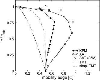
Figure 2: Mobility edge trajectory for the Anderson model calculated with KPM for a 3d-lattice (diamonds), and with AAT (circles), representing the distribution through a sample with $5\times 10^{4}$ elements. The crosses indicate points in the $(\omega,\gamma)$-plane, which correspond to delocalised states if sampled with $2.5\times 10^{7}$ elements. The dotted (dashed) line shows the mobility edge trajectory resulting from TMT (simplified TMT-variant).

Fig. 2 shows mobility edge trajectories calculated with AAT and KPM. Both trajectories show the same qualitative features. In contrast to KPM the AAT scheme does not suffer from limitations due to the finite geometric size of the system under consideration. Though the resolution which the distribution is sampled with in AAT is restricted by the finite size of the Monte-Carlo sample, this limitation can be easily overcome by increasing the sample size (cf. Fig. 1, 2). In principle this allows for an extremely precise determination of mobility edges within AAT.

Although both KPM and AAT construct the full distribution of the LDOS the localisation transition already manifests itself in a suitable moment thereof (e.g. the typical density of states). As a matter of course, this triggers the question whether the localisation problem can be treated by an effective theory using this moment as an (scalar and local) order parameter.

Indeed, the typical medium theory (TMT) [5] which is entirely based on the typical density of states is believed to capture the most basic effects of Anderson localisation, and has been recently applied to the Anderson-Hubbard model [6]. From a pragmatic point of view it is quite favorable to replace AAT by the simpler TMT. However, the typical density of states is no obvious choice for the order parameter. In contrast to what is sometimes claimed it provides no good approximation to the most probable value (cf. Fig. 1). So we tried to simplify even further and replaced the typical density of states with the minimal values of the LDOS calculated for the maximal value of the on-site potential $\epsilon_{i}$, i.e. $\epsilon_{i}=\pm\gamma/2$ for the box distribution. This means to incorporate only the maximal scattering contribution, originating from the deepest impurity. We can then calculate a mobility edge trajectory which, at a first glance, does equally well compared with the one resulting from TMT (cf. Fig. 2). Nevertheless, the two approaches fail to obtain the reentrant behaviour of the mobility edges. It seems that both TMT and our simplified TMT-variant do only capture localisation caused by deep impurities (“pushing states outside the band”), but not the subtle effects caused by quantum interference. Consistent with this interpretation the critical disorder predicted by these approaches is smaller than given by AAT. Therefore we come to the conclusion that the treatment of disordered systems within TMT might be inherently problematic.

To summarise: AAT is a theory of high precision for exponential localisation on the Bethe lattice which recovers all qualitative effects of exponential localisation on hypercubic lattices. The use of distributions in numerical treatments of Anderson localisation is further justified by a comparison to results obtained for 3d-hypercubic lattices. While localisation effects originating from local correlations are fully contained in AAT they are partially lost in averaged descriptions as TMT.

References

- [1] P. W. Anderson, Phys. Rev. 109, 1492 (1958).
- [2] R. Abou-Chacra, P. W. Anderson, and D. J. Thouless, J. Phys. C 6, 1734 (1973).
- [3] G. Schubert, A. Weiße, and H. Fehske, cond-mat/0309015 (2003).
- [4] F. X. Bronold, A. Alvermann, and H. Fehske, Phil. Mag. 84, 673 (2004).
- [5] V. Dobrosavljević, A. A. Pastor, and B. K. Nikolić, Europhys. Lett. 62, 76 (2003).
- [6] K. Byczuk, W. Hofstetter, and D. Vollhardt, cond-mat/0403765 (2004).