Efficient Algorithms for Sampling and Clustering of Large Nonuniform Networks

Abstract

We propose efficient algorithms for two key tasks in the analysis of large nonuniform networks: uniform node sampling and cluster detection. Our sampling technique is based on augmenting a simple, but slowly mixing uniform MCMC sampler with a regular random walk in order to speed up its convergence; however the combined MCMC chain is then only sampled when it is in its “uniform sampling” mode. Our clustering algorithm determines the relevant neighbourhood of a given node $u$ in the network by first estimating the Fiedler vector of a Dirichlet matrix with $u$ fixed at zero potential, and then finding the neighbourhood of $u$ that yields a minimal weighted Cheeger ratio, where the edge weights are determined by differences in the estimated node potentials. Both of our algorithms are based on local computations, i.e. operations on the full adjacency matrix of the network are not used. The algorithms are evaluated experimentally using three types of nonuniform networks: Dorogovtsev-Goltsev-Mendes “pseudofractal graphs”, scientific collaboration networks, and randomised “caveman graphs”.

1 Introduction

Two key tasks in the analysis of large natural networks, such as communication networks and social networks, are obtaining a uniform sample of nodes in the network, and determining the densely interconnected clusters of nodes. Uniform sampling is important e.g. for the purpose of estimating basic network characteristics such as the degree distribution, average path length, and clustering coefficient; it is, however, nontrivial to obtain a truly uniform random sample of nodes from a large, practically unobtainable network such as the WWW [13]. In this paper, we suggest an efficient approach for uniform sampling of undirected nonuniform graphs, using a construction that combines two types of random walks to produce one that mixes rapidly and still converges to the uniform distribution over the set of nodes.

We also discuss the problem of clustering nonuniform networks, i.e. the recognition of subgraphs where the nodes have relatively many edges among themselves and relatively few edges connecting them to the rest of the graph [16]. For large nonuniform networks, an effective clustering algorithm should scale at most linearly in the size of the graph, and for many applications, a method for determining the local cluster of a given source node will suffice, rather than a complete clustering of the entire graph. In this paper, we use approximate Fiedler vectors to determine potentials around a given source node, and then use the potentials to stochastically select an appropriate local cluster.

In Section 2, we present the MCMC construction for uniform sampling, and in Section 3 discuss experiments performed with the method. Section 4 discusses local clustering with Fiedler vectors. Finally, Section 5 summarises the work and addresses directions for further research.

2 An Efficient MCMC Method for Uniform Sampling

Let $G=(V,E)$ be a connected symmetric simple graph with $n$ nodes and $m$ edges. We denote the neighbourhood of node $i\in V$ by $\Gamma(i)=\{j\in V\mid(i,j)\in E\}$, and the degree of $i$ by $\deg(i)=|\Gamma(i)|$. It is well known (and easy to verify) that the regular random walk on $G$, with transition probabilities

$$p_{ij}=\left\{\begin{array}[]{ll}\displaystyle{\frac{1}{\deg(i)}},&\quad\text{if }j\in\Gamma(i),\\ 0,&\quad\text{otherwise,}\end{array}\right.$$ (1)

satisfies the detailed balance conditions

$$\forall i,\,j\in V:\pi_{i}\cdot p_{ij}=\pi_{j}\cdot p_{ji}$$ (2)

with respect to the distribution $\pi_{i}=\deg(i)/2m$, and hence this distribution, which we denote by $\pi_{\text{RW}}$, is stationary w.r.t. the walk [4, 14]. If $G$ is non-bipartite, then $\pi_{\text{RW}}$ is the unique equilibrium distribution. The chain (1) mixes rapidly, but the probability of obtaining any given node $i$ as a sample from it is proportional to the degree of $i$, and thus not uniform unless $G$ is regular.

A straightforward approach to uniform sampling [1] would be to augment the nodes of $G$ with virtual self-loops so as to make them all have the same degree $d=\max_{i\in V}\deg(i)$. This method, however, requires knowing the target degree $d$ ahead of time, and such global information is typically not available in many of the interesting applications. Moreover, this process may create some convergence anomalies in the case of highly nonuniform graphs $G$. Another alternative [13, 21] would be to postprocess a sample obtained from walk (1) in order to compensate for the bias in the stationary distribution $\pi_{\text{RW}}$. Such postprocessing, however, requires some a priori information on the number of burn-in steps needed before one can obtain a representative sample from $\pi_{\text{RW}}$, and the burn-in time again depends on the global structure of $G$.

We take a complementary approach, by starting from a somewhat more slowly mixing random walk on $G$ with a provably uniform stationary distribution, and then “accelerate” this walk by coupling it together with the chain (1); however we only sample the combined process when it is in the “uniform sampling” mode.

More precisely, we take as our starting point the following degree-balanced random walk on $G$, where the transition probabilities from node $i$ are inversely proportional to the degree of the target node $j$:

$$p_{ij}=\left\{\begin{array}[]{ll}\displaystyle\frac{1}{\deg(i)\cdot\deg(j)},&\text{ if }j\in\Gamma(i),\\ 1-\displaystyle\sum_{j\in\Gamma(i)}\displaystyle\frac{1}{\deg(i)\cdot\deg(j)},&\text{ if }j=i,\\ 0,&\text{ otherwise.}\end{array}\right.$$ (3)

It is simple to verify that the transition probabilities $p_{ij}$ given by (3) satisfy the detailed balance conditions with respect to the uniform distribution $\pi_{\text{ID}}(i)=1/n$, and hence $\pi_{\text{ID}}$ is a stationary distribution for this chain. (Note that in this case the equilibrium distribution is unique for any $G$ with more than two nodes, since any node $i$ with non-leaf neighbours has a self-loop probability of $p_{ii}>0$.)

However, this degree-balanced walk avoids visiting the high-degree nodes of a nonuniform graph, and so mixes relatively poorly in the graphs of most interest to us. A related problem is that the self-loop probabilities $p_{ii}$ are rather large for nodes with many high-degree neighbours.

Figure 1: A diagram of the mirror construction for two nodes $i$ and $j$ on the sampling side and their mirror nodes $i^{\prime}$ and $j^{\prime}$ on the mixing side.

In order to construct a sampling method that produces uniformly distributed samples but avoids the convergence problems of chain (3), we propose the following construction (cf. Figure 1): for each node $i\in V$ we create a “mirror node” $i^{\prime}$. The original nodes $i\in V$ are called the “sampling side” and the mirror nodes $i^{\prime}\in V^{\prime}$ are the “mixing side” of the augmented graph ($|V|=|V^{\prime}|=n)$. We continue to denote by $\deg(i)=\deg(i^{\prime})$ the degree of $i$ in the original graph $G$, i.e., ignoring the added edges that connect the two sides.

The transition probabilities on the sampling side follow those of the degree-balanced random walk; on the mixing side, a regular random walk is mimicked with minor modifications. The exact transition probabilities are defined as follows: let $\epsilon$ be a parameter satisfying $0<\epsilon<p_{ii}$ for all $i\in V$ — further restrictions on $\epsilon$ are discussed later in this section. Fix all the sampling-to-mixing transition probabilities $p_{ii^{\prime}}$ to $\epsilon$. On the sampling side, subtract $\epsilon$ from each $p_{ii}$ and give all other transition probabilities the values they would have in the degree-balanced walk. On the mixing side, denote the probability of moving back to the sampling side from nodes $i^{\prime}$ by $p_{i^{\prime}i}=\epsilon^{\prime}_{i}$. Let $\delta$ be a parameter (to be determined later) such that $\delta\geq\epsilon^{\prime}_{i}$ for all $i^{\prime}\in V^{\prime}$. Add to each node $i^{\prime}\in V^{\prime}$ a self-loop with transition probability $p_{i^{\prime}i^{\prime}}=\delta-\epsilon^{\prime}_{i}$, and divide the remaining probability mass $1-\delta$ evenly among the neighbours of $i^{\prime}$ as in a regular random walk, i.e. assign $p_{i^{\prime}j^{\prime}}=(1-\delta)\frac{1}{\deg(i)}$ for each $j^{\prime}\in\Gamma(i^{\prime})\setminus\{i\}$.

We claim that the stationary distribution of such a combination walk is a weighted combination of the distributions $\pi_{\text{ID}}$ and $\pi_{\text{RW}}$, such that an $\alpha$-fraction of the time the chain is in a state $i\in V$, and an $(1-\alpha)$-fraction of the time is spent within $V^{\prime}$:

$$\pi_{C}(x)=\left\{\begin{array}[]{ll}\alpha\cdot\pi_{\text{ID}}(x)=\alpha\cdot\frac{1}{n},&\text{ if }x=i\in V,\\ (1-\alpha)\cdot\pi_{\text{RW}}(x)=(1-\alpha)\cdot\frac{deg(i)}{2m},&\text{ if }x=i^{\prime}\in V^{\prime}.\\ \end{array}\right.$$ (4)

To verify the claim it suffices to check the detailed balance conditions (2) for the above construction. There are three cases to consider: (i) transitions within $V$, (ii) transitions within $V^{\prime}$, and (iii) transitions between $V$ and $V^{\prime}$.

The first two cases are essentially the same as those considered in the settings of the balanced and regular random walks, respectively: only some constant coefficients ($\alpha$, $(1-\alpha)$, $(1-\delta)$) appear on both sides of the balance equations and cancel out. This leaves us with the third type: here the requirement is that any transitions between a node $i\in V$ and its mirror node $i^{\prime}\in V^{\prime}$ satisfy $\pi_{C}(i)\cdot p_{ii^{\prime}}=\pi_{C}(i^{\prime})\cdot p_{i^{\prime}i}$, i.e. that

$$\alpha\frac{1}{n}\cdot\epsilon=(1-\alpha)\frac{\deg(i)}{2m}\cdot\epsilon^{\prime}_{i},\quad\text{for all $i\in V$.}$$ (5)

These equations can be satisfied by solving for the transition probabilities $\epsilon^{\prime}_{i}$, once values for the parameters $\alpha$ and $\epsilon$ have been chosen:

$$\epsilon^{\prime}_{i}=\frac{2m\alpha\epsilon}{n(1-\alpha)\deg(i)}=\frac{2m}{n}\cdot\frac{\alpha}{(1-\alpha)}\epsilon\deg(i)^{-1},$$ (6)

where $\frac{2m}{n}=\bar{k}$ is the average degree of nodes in $G$. As a probability, $\epsilon^{\prime}_{i}$ must be at most one for all $i\in V$. This yields an additional restriction on the parameter $\epsilon$:

$$\epsilon\leq\frac{n}{2m}\cdot\frac{1-\alpha}{\alpha}\deg(i)=\frac{1}{\bar{k}}\cdot\frac{1-\alpha}{\alpha}\deg(i),\quad\text{for all $i\in V$}.$$ (7)

Since $\deg(i)\geq 1$ for all $i\in V$, it suffices to choose $\epsilon\leq\bar{k}^{-1}\frac{1-\alpha}{\alpha}$. For a (nonuniform) graph, averaging over a regular random walk will quickly give a positively biased estimate for $\bar{k}$ that can be used to bound $\epsilon$; note that many nonuniform networks have a modest average degree, despite the existence of a few extremely high-degree nodes.

In an implementation of the above sampler one does not of course make explicit copies of the node sets, but rather uses a state flag that indicates which set of transition probabilities should be applied. All the transition probabilities are locally computable at each node $i$, if the parameters $\epsilon$ and $\alpha$ are given, and the degrees of both the node $i$ and its neighbours in $\Gamma(i)$ are accessible. The dependency of $\epsilon^{\prime}_{i}$ on the parameter $\alpha$ and the average degree $\bar{k}=2m/n$ can be resolved by simply always setting $\epsilon^{\prime}_{i}=\displaystyle\frac{\epsilon}{\deg(i)}$, which implicitly fixes the relationship

$$\frac{\alpha}{1-\alpha}\cdot\displaystyle\frac{2m}{n}=1\Rightarrow\alpha=\displaystyle\frac{1}{\bar{k}+1}.$$ (8)

This implies by equation (7) the condition $\epsilon\leq 1$, which is a natural restriction on $\epsilon$. By this choice of $\epsilon^{\prime}_{i}$ we also have $\epsilon^{\prime}_{i}\leq\epsilon$ for all $i\in V$, and may thus set $\delta=\epsilon$, completing the definition of the transition probabilities on the mixing side.

Figure 2: The DGM pseudo-fractal graphs $G_{t}$ (adapted from [8]). Newly added nodes are drawn white.

3 Sampling experiments

In this section, we report on experiments using the above sampler construction on both artificial networks with known properties (so called “pseudofractal graphs” of Dorogovtsev, Goltsev, and Mendes [8]), and scientific collaboration networks of $n=$ 503 and $n=$ 5,909 mathematicians and computer scientists, with total number of coauthorships $m=$ 828 and $m=$ 13,510 respectively (subgraphs of the network constructed in [24]).

In the deterministic scale-free network model of Dorogovtsev, Goltsev, and Mendes [8] (based on [2]), the initial graph $G_{-1}=(V_{-1},E_{-1})$ consists of two nodes $v$ and $w$ and an edge $(v,w)$. At each generation $t\geq 0$ of the generative process, per each edge $(u,v)\in E_{t-1}$, a new node $w$ is added together with edges $(u,w)$ and $(v,w)$. (See Figure 2 for an illustration of the first five generations.) The resulting graphs $G_{t}$ have an almost constant average degree of $\bar{k}_{t}=4(1+3^{-t})$, yet a power-law distribution of node degrees according to $n_{t}(d)=3^{t+1}d^{-\log_{2}3}$.

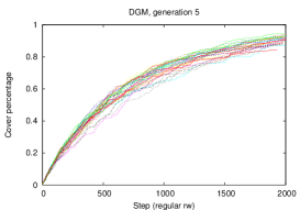
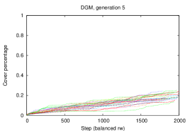
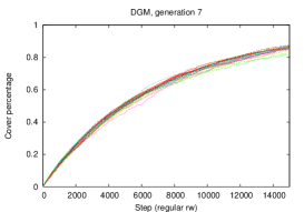
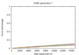
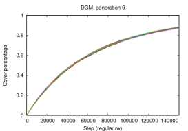
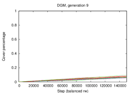
Figure 3: The coverage achieved by the regular (top row) and the degree-balanced walks at each step for DGM graphs of generations 5, 7, and 9. In each plot, 30 independent walks are shown.

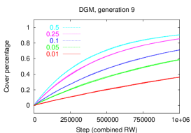
Figure 4: The coverage achieved by the combination random walk on a ninth generation DGM graph for different values of $\epsilon$.

As a first indication of the behaviour of various sampling strategies, Figures 3 and 4 present plots of the percentage of graph covered versus length of the walk, for DGM networks $G_{5}$, $G_{7}$ and $G_{9}$. Note that the combination walks sample fewer nodes during a walk of a given length than the others, as it does not record samples during the mixing phase. The tendency of the degree-balanced method to unwanted locality is quite evident in Figure 3.

In another set of experiments, we estimated the rate of convergence of the above discussed random walks to their respective stationary distributions. If $\pi_{t}$ is the distribution of a random walk after $t$ steps, and $\pi$ is its stationary distribution, the total variation distance between the two is defined as [4, 14]:

$$\Delta(t)=\max_{S\subseteq V}|\pi_{t}(S)-\pi(S)|=\frac{1}{2}\sum_{i\in V}|\pi_{t}(i)-\pi(i)|.$$ (9)

We estimate this quantity by running $k$ independent instantiations of a given random walk starting from the same start node, and looking at the state distributions at time $t$ of the instantiations. For definiteness, let us consider the case where the stationary distribution is uniform, with $\pi(i)=1/n$ for all $i\in V$. Denoting by $f_{t}(i)$ the number of instantiated walks that are visiting node $i$ at time $t$, a conservative estimate of the total variation distance at time $t$ can then be computed as [5]:

$$\Delta_{\text{est}}(t)=1-\sum_{i=1}^{n}\min\bigg{\{}\frac{f_{t}(i)}{k},\,\frac{1}{n}\bigg{\}}.$$ (10)

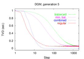
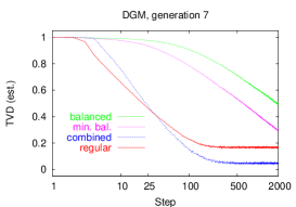
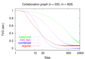
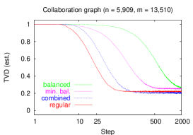
Figure 5: Values of $\Delta_{\text{est}}(t)$ for the regular, degree-balanced, combination, and Metropolis-Hastings (“minimum-balanced”) random walks over a set of 15,000 independent walks in two DGM graphs and two collaboration graphs, all starting from a fixed node, initially chosen at random. Note logarithmic scale on the time axis.

Figure 5 shows the time evolution of these estimates for the regular, balanced, combination random walks and the Metropolis-Hastings walk of [3] in DGM graphs of generations five and seven, and for the two collaboration graphs of $n=$ 503 and $n=$ 5,909 scientists. The stationary distribution for the regular walk is taken to be the degree-proportional distribution $\pi_{\text{RW}}$, and for the three other walks the uniform distribution $\pi_{\text{ID}}$. For the combination walk, only those instantiated walks that are on the sampling side at any given time step are included in computing the corresponding estimate. The plots illustrate quite graphically (particularly in the case of the heavy-tailed DGM graphs) that the convergence behaviour of the combination walk is qualitatively similar to that of the regular walk, whereas both the pure balanced walk and the Metropolis-Hastings walk converge noticeably more slowly.

4 Local clustering by approximate Fiedler vectors

Another key task in the analysis of natural networks is finding clusters of densely interconnected nodes. Most of the existing literature on this topic (see [19] for a survey) considers the task of finding an ideal complete clustering of a given graph. This is, however, often unnecessary and in any case infeasible in the case of really large networks such as the WWW. (The fastest complete algorithms can currently deal with networks containing up to maybe a few millions of nodes [15, 18, 19].) In many cases it would be sufficient to know the relevant cluster of a given source node, or maybe a group of nodes. Some recent papers, such as [23, 25] address also this more limited goal.

In [23, 24], a parameter-free local clustering quality measure is optimised using simulated annealing: the computational effort needed to obtain the cluster of a given source node is quite modest (and, most importantly, independent of the total size of the network), and the results seem to be quite robust w.r.t. variations in the annealing process. In [25], the clustering task is formulated as a problem of determining voltage levels in an electrical circuit with unit resistances corresponding to the edges of the original network. The source node is fixed at a high voltage value and a randomly selected target node at low voltage; an approximate solution to the Kirchhoff equations is computed by an iteration scheme, and the eventual cluster of the source node is deemed to consist of those nodes whose voltages are “close” to the high value. The possibility that the target node is accidentally selected from within the natural cluster of the source node is decreased by repeating the experiment some small number of times and determining cluster membership by majority vote.

This electrical circuit analogue appears to have been first suggested in [19], where however the aim is to compute a complete clustering of a given network by considering all possible source-target pairs, and for each pair solving the Kirchhoff equations exactly by explicitly inverting the corresponding Laplacian matrix. (We note that since solutions of the Kirchhoff equations can be decomposed in terms of the eigenvectors of the circuit graph Laplacian, this method is a variant of the much-studied spectral partitioning techniques [9, 10, 11, 12, 16, 20, 22]. A distributed algorithm for spectral analysis, possibly suited for large networks, is proposed in [17]. A fundamental reference is [6].)

We continue the analogue of representing cluster membership values as physical potentials, but eliminate the unnatural choice of random “target” nodes by basing our model on diffusion in an unbounded medium rather than an electrical closed-circuit model. Thus, we fix the source node $i$ at a constant potential level, which we choose to be zero, and find an eigenvector $u$ corresponding to the smallest eigenvalue $\sigma_{1}$ of the respective Dirichlet matrix, i.e. the Laplacian matrix of the network with row and column $i$ removed [6, 7]. This eigenvector $u$, called the (Dirichlet-)Fiedler vector of the graph, will now (hopefully) assign potential values $u(j)$ close to 0 for nodes $j$ that are within a densely interconnected neighbourhood of the source node $i$, and larger values for nodes that have sparser connections to the source. (The method obviously generalises to starting from a larger set of source nodes, if desired.)

Since we wish to develop a local algorithm, and not deal with the full adjacency matrix of the network, we approach the computation of the Fiedler vector $u$ via minimising the Rayleigh quotient [6, 7]:

$$\sigma_{1}\quad=\quad\inf_{u}\frac{\sum_{j\sim k}(u(j)-u(k))^{2}}{\sum_{j}u(j)^{2}},$$ (11)

where the infimum is computed over vectors $u$ satisfying the Dirichlet boundary condition of having $u(i)=0$ for the source node(s). (The notation $j\sim k$ is an abbreviation for $(j,k)\in E$.) Furthermore, since we are free to normalise our eventual Fiedler vector to any length we wish, we can constrain the minimisation to vectors $u$ that satisfy, say, $\|u\|^{2}_{2}=n=|V|$. Thus, the task becomes one of finding a vector $u$ that satisfies:

$$u\quad=\quad\mbox{argmin}\bigg{\{}\sum_{j\sim k}(u(j)-u(k))^{2}\;\mid\;u(i)=0,\;\|u\|_{2}^{2}=n\bigg{\}}.$$ (12)

We can solve this task approximately by reformulating the requirement that $\|u\|_{2}^{2}=n$ as a “soft constraint” with weight $c>0$, and minimising the objective function

$$f(u)\quad=\quad\frac{1}{2}\sum_{j\sim k}(u(j)-u(k))^{2}+\frac{c}{2}\cdot\big{(}n-\sum_{j}u(j)^{2}\big{)}$$ (13)

by gradient descent. Since the partial derivatives of $f$ have the simple form

$$\frac{\partial f}{\partial u(j)}\quad=\quad-\sum_{k\sim j}u(k)+(\deg(j)-c)\cdot u(j),$$ (14)

the descent step can be computed locally at each node, based on information about the $u$-estimates at the node itself and its neighbours:

$$\tilde{u}_{t+1}(j)\quad=\quad\tilde{u}_{t}(j)+\delta\cdot\big{(}\sum_{k\sim j}\tilde{u}(k)-(\deg(j)-c)\cdot\tilde{u}(j)\big{)},$$ (15)

where $\delta>0$ is a parameter determining the speed of the descent. Assuming that the natural cluster of node $i$ is small compared to the size of the full network, the normalisation $\|u\|_{2}^{2}=n$ entails that most nodes $j$ in the network will have $u(j)\approx 1$. Thus the descent iterations (15) can be started from an initial vector $\tilde{u}_{0}$ that has $\tilde{u}_{0}(i)=0$ for the source node $i$ and $\tilde{u}_{0}(k)=1$ for all $k\neq i$. The estimates need then to be updated at time $t>0$ only for those nodes $j$ that have neighbours $k\sim j$ such that $\tilde{u}_{t-1}(k)<1$.

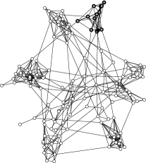
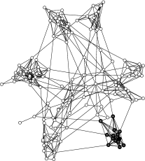
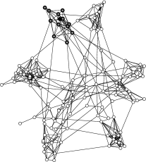
Figure 6: Three local Fiedler clusters in a caveman graph of 138 nodes.

Figure 6 represents the results of such approximate Fiedler vector calculations in the case of a slightly randomised “caveman” network of 138 nodes, starting from three different source nodes. For visual effect, the nodes are colour-coded so that dark colours correspond to small approximated Fiedler potential values, with the source node in each case coloured black. The parameter values used in this case were $c=0.1$, $\delta=0.05$.

Visually, the clusters in e.g. Figure 6 look reasonable; in practice, however, we need to determine the cluster boundaries automatically. One possibility would be to threshold the potentials as in [25], but we prefer not to introduce any additional instance-specific parameters to the algorithm. A natural alternative is to find a set of nodes $S$ that contains the source node $i$ and minimises some weighted Cheeger ratio [6, p. 35]:

$$h_{w}(S)\quad=\quad\frac{\sum_{j\in S}\sum_{k\sim j,k\not\in S}w(j,k)}{\sum_{j\in S}\sum_{k\sim j}w(j,k)},$$ (16)

where $w(j,k)$ is an appropriate nonnegative edge weight function. In our experiments, edge weights determined as $w(j,k)=(|u(j)-u(k)|)^{-1}$ seem to lead to natural clusters in different types of networks, and are also intuitively appealing. In Figure 6, we have indicated the nodes selected by this heuristic as belonging to each cluster by circles with thick boundaries. The minimisation of the cluster cost function (16) was here performed by a local simulated annealing process similar to the one used in [23, 24].

5 Conclusions and Further Work

In this paper we presented two methods to help analyse properties of large nonuniform graphs: a uniform sampling construction and a local method for clustering based on approximate Fiedler vectors. According to our experiments, both approaches are well-behaving and conform to the intuition that arises from their analytical properties.

As future work, we will look into more general constructions for rapidly mixing uniform MCMC samplers; one direction might be to combine the regular random walk with alternative slow uniform samplers, such as those of [3]. Accuracy of the estimates of natural network network characteristics based on our pseudo-uniform samples should also be assessed. Both the sampling and the clustering algorithms should also be extended to work on directed graphs, in order to deal with interesting natural networks such as the WWW.

Acknowledgments

We thank most appreciatively Mr. Kosti Rytk nen for providing us with his automatic graph drawing tool used to produce the diagrams in Figure 6.

References

- [1] Z. Bar-Yossef, A. Berg, S. Chien, J. Fakcharoenphol, and D. Weitz. Approximating aggregate queries about Web pages via random walks. In Proceedings of the 26th International Conference on Very Large Data Bases (VLDB’00), pages 535–544, Palo Alto, CA, 2000. Morgan Kaufmann.
- [2] A.-L. Barabási, E. Ravasz, and T. Vicsek. Deterministic scale-free networks. Physica A, 299(3–4):559–564, Oct. 15 2001, cond-mat/0107419.
- [3] S. Boyd, P. Diaconis, and L. Xiao. Fastest mixing Markov chain on a graph, 2004. Submitted for publication.
- [4] P. Br maud. Markov Chains, Gibbs Fields, Monte Carlo Simulation, and Queues. Springer-Verlag, New York, NY, 1999.
- [5] S. P. Brooks, P. Dellaportas, and G. O. Roberts. An approach to diagnosing total variation convergence of MCMC algorithms. Journal of Computational and Graphical Statistics, 6:251–265, 1997.
- [6] F. R. K. Chung. Spectral Graph Theory. American Mathematical Society, Providence, RI, 1997.
- [7] F. R. K. Chung and R. B. Ellis. A chip-firing game and Dirichlet eigenvalues. Discrete Mathematics, 257:341–355, 2002.
- [8] S. N. Dorogovtsev, A. V. Goltsev, and J. F. F. Mendes. Pseudofractal scale-free web. Physical Review E, 65(6):066122, June 2002, cond-mat/0112143.
- [9] M. Fiedler. Algebraic connectivity of graphs. Czechoslovak Mathematical Journal, 23:298–305, 1973.
- [10] M. Fiedler. A property of eigenvectors of nonnegative symmetric matrices and its application to graph theory. Czechoslovak Mathematical Journal, 25:619–633, 1975.
- [11] C. Gkantsidis, M. Mihail, and E. Zegura. Spectral analysis of Internet topologies. In Proceedings of the 22nd Annual Joint Conference of the IEEE Computer and Communications Societies (INFOCOM’03), pages 364–374, New York, NY, 2003. IEEE.
- [12] S. Guattery and G. L. Miller. On the quality of spectral separators. SIAM Journal on Matrix Analysis and Applications, 19(3):701–719, 1998.
- [13] M. R. Henzinger, A. Heydon, M. Mitzenmacher, and M. Najork. On near-uniform URL sampling. In Proceedings of the 9th International World Wide Web Conference, pages 295–308, 2000. URL: http://www9.org/w9cdrom/88/88.html.
- [14] O. Häggström. Finite Markov Chains and Algorithmic Applications. Cambridge University Press, Cambridge, U.K., 2002.
- [15] J. Hopcroft, O. Khan, B. Kulis, and B. Selman. Natural communities in large linked networks. In Proceedings of the 9th ACM SIGKDD International Conference on Knowledge Discovery and Data Mining, pages 541–546, New York, NY, 2003. ACM.
- [16] R. Kannan, S. Vempala, and A. Vetta. On clusterings: Good, bad and spectral. Journal of the ACM, 51(3):497–515, 2004.
- [17] D. Kempe and F. McSherry. A decentralized algorithm for spectral analysis. In Proceedings of the 36th ACM Symposium on Theory of Computing (STOC’04), New York, NY, 2004. ACM.
- [18] M. E. J. Newman. Fast algorithm for detecting community structure in networks. Technical Report, arXiv.org, Sept. 2003, cond-mat/0309508.
- [19] M. E. J. Newman and M. Girvan. Finding and evaluating community structure in networks. Physical Review E, 69:026113, 2004, cond-mat/0308217.
- [20] A. Pothen, H. D. Simon, and K. P. Liou. Partitioning sparse matrices with egenvectors of graphs. SIAM Journal of Matrix Analysis and Applications, 11:430–452, 1990.
- [21] P. Rusmevichientong, D. M. Pennock, S. Lawrence, and C. Giles. Methods for sampling pages uniformly from the World Wide Web, 2001. AAAI 2001 Fall Symposium on Using Uncertainty Within Computations. URL: http://www-users.cs.york.ac.uk/~tw/fall/Proceedings/.
- [22] D. A. Spielman and S.-H. Teng. Spectral partitioning works: planar graphs and finite element meshes. In Proceedings of the 37th IEEE Symposium on Foundations of Computing (FOCS’96), pages 96–105, Los Alamitos, CA, 1996. IEEE Computer Society.
- [23] S. E. Virtanen. Clustering the Chilean Web. In Proceedings of the First Latin American Web Congress, pages 229–231, Los Alamitos, CA, 2003. IEEE Computer Society.
- [24] S. E. Virtanen. Properties of nonuniform random graph models. Research Report A77, Helsinki University of Technology, Laboratory for Theoretical Computer Science, Espoo, Finland, May 2003. URL: http://www.tcs.hut.fi/Publications/info/bibdb.HUT-TCS-A77.shtml.
- [25] F. Wu and B. A. Huberman. Finding communities in linear time: a physics approach. The European Physics Journal B, 38:331–338, 2004, cond-mat/0310600.