Orbital and magnetic transitions in geometrically-frustrated vanadium spinels
– Monte Carlo study of an effective spin-orbital-lattice coupled model –

Abstract

We present our theoretical and numerical results on thermodynamic properties and the microscopic mechanism of two successive transitions in vanadium spinel oxides $A$V₂O₄ ($A$=Zn, Mg, or Cd) obtained by Monte Carlo calculations of an effective spin-orbital-lattice model in the strong correlation limit. Geometrical frustration in the pyrochlore lattice structure of V cations suppresses development of spin and orbital correlations, however, we find that the model exhibits two transitions at low temperatures. First, a discontinuous transition occurs with an orbital ordering assisted by the tetragonal Jahn-Teller distortion. The orbital order reduces the frustration in spin exchange interactions, and induces antiferromagnetic correlations in one-dimensional chains lying in the perpendicular planes to the tetragonal distortion. Secondly, at a lower temperature, a three-dimensional antiferromagnetic order sets in continuously, which is stabilized by the third-neighbor interaction among the one-dimensional antiferromagnetic chains. Thermal fluctuations are crucial to stabilize the collinear magnetic state by the order-by-disorder mechanism. The results well reproduce the experimental data such as transition temperatures, temperature dependence of the magnetic susceptibility, changes of the entropy at the transitions, and the magnetic ordering structure at low temperatures. Quantum fluctuation effect is also examined by the linear spin wave theory at zero temperature. The staggered moment in the ground state is found to be considerably reduced from saturated value, and reasonably agrees with the experimental data.

I Introduction

Geometrical frustration in strongly-correlated systems is one of the long-standing problems in condensed matter physics. Frustration suppresses a formation of a simpleminded long-range order and results in nearly-degenerate ground-state manifolds of a large number of different states. Many well-known examples are found in frustrated antiferromagnetic (AF) spin systems. There, all the antiparallel spin conditions between interacting pairs cannot be satisfied at the same time because closed loops contain an odd number of sites. The degeneracy due to the frustration yields nontrivial phenomena such as complicated ordering structures, spin liquid states, and glassy states. Diep1994 ; Liebmann1986 Besides the spin degree of freedom, charge ordering phenomena are also much affected by the geometrical frustration. Anderson1956 Quantum and thermal fluctuations play important roles in these systems, which are difficult to handle in a controllable manner.

Figure 1: Cubic unit cell of the lattice structure of vanadium spinel oxides $A$V₂O₄. (a) The pyrochlore lattice of vanadium cations (red balls). (b) The 3D edge-sharing network of VO₆ octahedra. Oxygen ions are on the corners of octahedra. Tetrahedral $A$ sites are omitted.

Pyrochlore lattice is a typical example of the geometrically-frustrated structures, and it consists of a three-dimensional (3D) network of corner-sharing tetrahedra as shown in Fig. 1 (a). Spin systems on the pyrochlore lattice have been intensively studied. Liebmann1986 ; Canals2000 ; Harris1991 ; Tsunetsugu2001 ; Koga2001 ; Berg2003 ; Reimers1991 ; Moessner1998 In particular, for quantum $S=1/2$ spin systems with only nearest-neighbor interactions, it is predicted that a macroscopic number of singlet states lie inside the singlet-triplet gap. Canals2000 Several types of symmetry breakings are predicted within the singlet subspace, e.g., dimer/tetramer ordering, but without magnetic long-range ordering. Harris1991 ; Tsunetsugu2001 ; Koga2001 ; Berg2003 Antiferromagnetic (AF) classical spin systems on the pyrochlore lattice are also believed to show no long-range ordering at any temperature. Liebmann1986 ; Reimers1991 ; Moessner1998 Due to the three dimensionality and the large unit cell (16 sites in the cubic unit cell), pyrochlore systems remain a big challenge to theoreticians and are still far from comprehensive understanding.

We can find many pyrochlore systems in real compounds. Most typically, pyrochlore systems are realized in so-called $B$ spinel oxides, where only $B$-site cations are magnetic in the general chemical formula $AB_{2}$O₄. Figure 1 (b) shows the $B$ spinel structure, which consists of a network of edge-sharing $B$O₆ octahedra. $B$ cation is shown by ball in center of each octahedron, and octahedron corners are occupied by oxygen ions, while nonmagnetic $A$-site cations are not shown for simplicity. With omitting oxygen ions on the corners of the octahedra, one obtains the pyrochlore lattice of $B$ cations in Fig. 1 (a).

In this paper, we will investigate insulating vanadium spinel oxides, $A$V₂O₄ with divalent $A$-site cations such as Zn, Mg, or Cd. In these compounds, each V³⁺ cation has two $3d$ electrons in a high-spin state by the Hund’s-rule coupling, and they are Mott insulators. Muhtar1988 Thus, we may consider that pyrochlore spin systems with $S=1$ are realized. Curie-Weiss temperature is estimated from the magnetic susceptibility as $|\Theta_{\rm CW}|\sim 1000$K, and any long-range ordering does not occur down to significantly lower temperatures than $|\Theta_{\rm CW}|$ due to the geometrical frustration. Muhtar1988 For instance, in ZnV₂O₄, a structural phase transition occurs at $T_{\rm c1}\simeq 50$K from the high-temperature cubic phase to the low-temperature tetragonal phase with a flattening of VO₆ octahedra in the $c$ direction. Ueda1997 Successively, an AF transition occurs at $T_{\rm c2}\simeq 40$K. Ueda1997 Neutron scattering experiments revealed that the AF ordering structure below $T_{\rm c2}$ is a collinear one which consists of the staggered AF chains in the $ab$ planes stacking in the $c$ direction with a four-times period as up-up-down-down-$\cdot\cdot\cdot$ as shown in Fig. 2. Niziol1973 ; Izyumov1979 These two successive transitions are commonly seen in compounds MgV₂O₄ and CdV₂O₄. Mamiya1997 ; Nishiguchi2002 This indicates that the degenerate ground-state manifolds in the pyrochlore systems are lifted at low temperatures in some manner.

Figure 2: Spin ordering structure proposed for ZnV₂O₄ on the basis of the neutron scattering results. The ordering pattern consists of staggered AF chains in the $ab$ plane (red solid lines) which stack with a four-times period in the $c$ direction as up-up-down-down-$\cdot\cdot\cdot$ (blue dashed lines). (b) Projection of (a) from the $z$ direction. Symbols of $+$ and $-$ denote the up and down spins, respectively.

A few years ago, Yamashita and Ueda proposed a scenario to explain the mechanism of the transitions in $A$V₂O₄. Yamashita2000 Their approach is based on a valence-bond-solid picture for $S=1$ spins and takes account of the coupling to Jahn-Teller (JT) lattice distortions. They claimed that the first transition at $T_{\rm c1}$ is due to the JT effect which lifts the degeneracy of the spin-singlet local ground states at each tetrahedron unit. This scenario based on the spin-JT coupling is appealing, however, some difficulty still remains. The problem is that it is difficult to explain the magnetic transition at a lower temperature $T_{\rm c2}$. In this approach, a finite energy gap is assumed between the spin-singlet ground-state subspace and the spin-triplet excitations, and a low-energy effective theory is derived to describe a phase transition within the spin-singlet subspace. High-energy excitations with total spin $S\neq 0$ are already traced out at the starting point, and therefore their effective model has no chance to describe the AF ordering within their theory.

A similar JT scenario was also examined for classical spin systems. Tchernyshyov2002 In this case, although the problem to have AF order does not exist, there is another difficulty to explain the following generic difference from chromium family of $A$Cr₂O₄ ($A$=Zn, Mg, or Cd). These chromium oxides are also $B$ spinels and magnetic Cr cations constitute a pyrochlore lattice. However, in contrast to the two transitions in vanadium compounds, the chromium compounds exhibit only one transition, i.e., the AF order appears simultaneously with the structural transition. Kagomiya2002 ; Rovers2002 This clear difference is generic, being independent of divalent $A$ cations, and ascribed to the difference of magnetic cations V³⁺ and Cr³⁺, which cannot be explained by the classical spin approach based on the spin-JT effect unless there exists essential difference in the model parameters between the two families.

Therefore, these spin-JT type theories appear to be insufficient to explain the mechanism of two transitions in vanadium spinels $A$V₂O₄. These insulating compounds are undoped states of LiV₂O₄ which exhibits a unique heavy fermion behavior. Kondo1997 ; Urano2000 The origin of the mass enhancement is still controversial between the scenario based on the Kondo effect Anisimov1999 ; Singh1999 ; Nekrasov2003 and the scenario of strong correlations with the geometrical frustration. Eyert1999 ; Matsuno1999 ; Fujimoto2001 ; Tsunetsugu2002 ; Yamashita2003 Since the doping of Li shows systematic changes of magnetic Muhtar1988 and transport properties, Kawakami1986 as well as the phase diagram, Ueda1997 ; Onoda1997 understanding of undoped materials may give a starting point to discuss the doped state in LiV₂O₄. Therefore, it is also highly desired to clarify the mechanism of orderings in the undoped compounds $A$V₂O₄.

The generic difference between vanadium and chromium spinels mentioned above suggests an importance of $t_{2g}$ orbital degrees of freedom. In the case of chromium spinels, each Cr³⁺ cation has three electrons in threefold $t_{2g}$ levels and large Hund’s-rule coupling leads to a high-spin state, and therefore, there is no orbital degree of freedom. On the contrary, in the case of vanadium spinels, since each V³⁺ cation has two electrons, the orbital degree of freedom is active. With taking account of this $t_{2g}$ orbital degeneracy, the authors have derived an effective spin-orbital-lattice coupled model in the strong correlation limit and investigated it by mean-field type arguments. Tsunetsugu2003 A reasonable scenario was obtained, but discussions were limited to a qualitative level. In order to investigate temperature dependences of physical properties semiquantitatively accurate enough to be compared with experimental data, we need more elaborate analysis.

In the present study, we will investigate thermodynamic properties of the effective spin-orbital-lattice model derived by the authors in Ref. Tsunetsugu2003, by extensive Monte Carlo (MC) calculations. We will show that this model indeed exhibits two successive transitions in a reasonable parameter range, and clarify the microscopic mechanism of these transitions in detail. First, an orbital order appears with the tetragonal JT distortion which flattens VO₆ octahedra. This orbital order reduces magnetic frustration partially, and enhances AF spin correlations in one-dimensional (1D) chains in the $ab$ planes. At a lower temperature, the third-neighbor exchange interaction and thermal fluctuations align these 1D AF chains coherently, and stabilize a 3D collinear AF order. With comparing numerical results of physical quantities with experimental data, we will show that our theory captures essential physics at low temperatures in the vanadium spinels $A$V₂O₄.

This paper is organized as follows. In Sec. II, we introduce the effective spin-orbital-lattice coupled model, and briefly summarize the mean-field arguments discussed in Ref. Tsunetsugu2003, . Realistic parameter values and MC method are also described. In Sec. III, we show numerical results in comparison with experimental data. We then make several remarks, in particular, on comparisons with experimental results and other theoretical proposals in Sec. IV. Section V is devoted to summary.

II Model and Method

II.1 Effective spin-orbital-lattice model

In the present study, we will investigate thermodynamic properties of the spin-orbital-lattice coupled model which is proposed by the authors in Ref. Tsunetsugu2003, . The Hamiltonian consists of two terms as

$$H=H_{\rm SO}+H_{\rm JT}.$$ (1)

The first term describes exchange interactions in spin and orbital degrees of freedom and the second term is for orbital-lattice couplings of the Jahn-Teller type.

The spin-orbital Hamiltonian $H_{\rm SO}$ is derived from a multiorbital Hubbard model with threefold $t_{2g}$ orbital degeneracy by the perturbation in the strong correlation limit. Kugel1973 The starting $t_{2g}$ Hubbard model is given in the form

$$H_{\rm Hub}=\sum_{i,j}\sum_{\alpha,\beta}\sum_{\tau}[t_{\alpha\beta}(\mbox{\boldmath$r$}_{i}-\mbox{\boldmath$r$}_{j})c_{i\alpha\tau}^{\dagger}c_{j\beta\tau}+{\rm H.c.}]$$

$$\quad+\frac{1}{2}\sum_{i}\sum_{\alpha\beta,\alpha^{\prime}\beta^{\prime}}\sum_{\tau\tau^{\prime}}U_{\alpha\beta,\alpha^{\prime}\beta^{\prime}}c_{i\alpha\tau}^{\dagger}c_{i\beta\tau^{\prime}}^{\dagger}c_{i\beta^{\prime}\tau^{\prime}}c_{i\alpha^{\prime}\tau},$$ (2)

where $i,j$ and $\tau,\tau^{\prime}$ are site and spin indices, respectively, and $\alpha,\beta=1$ ($d_{yz}$), $2$ ($d_{zx}$), $3$ ($d_{xy}$) are orbital indices. The first term of $H_{\rm Hub}$ is the electron hopping, and the second term describes Coulomb interactions, for which we use the standard parametrizations, note2

$$U_{\alpha\beta,\alpha^{\prime}\beta^{\prime}} = U^{\prime}\delta_{\alpha\alpha^{\prime}}\delta_{\beta\beta^{\prime}}+J_{\rm H}(\delta_{\alpha\beta^{\prime}}\delta_{\beta\alpha^{\prime}}+\delta_{\alpha\beta}\delta_{\alpha^{\prime}\beta^{\prime}}),$$ (3)

$$U = U^{\prime}+2J_{\rm H}.$$ (4)

We do not include here the relativistic spin-orbit coupling and the trigonal distortion in the model (2). Effects of these neglected elements will be discussed in Sec. IV.2 and E.

Considering the vanadium spinel oxides are insulators, it is reasonable to start from the strong correlation limit and treat the hopping term as perturbation. The unperturbed states are atomic eigenstates with two electrons on each V cation in a high-spin state. As for the perturbation part, on the basis of the tight-binding fit for the band structure Matsuno1999 (see Sec. II.2), we take account of hopping integrals of $\sigma$ bonds for nearest-neighbor pairs, $t_{\sigma}^{\rm nn}$, and for third-neighbor pairs, $t_{\sigma}^{\rm 3rd}$, as shown in Fig. 3. Note that the third-neighbor pair corresponds to the next nearest-neighbor pair along each chain. The hopping integral between second-neighbor pairs (the gray arrow in Fig. 3) is expected to be small because of the geometry of the pyrochlore lattice, note4 and moreover the exchange interaction derived from it is frustrated.

Figure 3: Hopping integrals for the $\sigma$ bonds; $t_{\sigma}^{\rm nn}$ and $t_{\sigma}^{\rm 3rd}$ are for the nearest-neighbor sites and for the third-neighbor sites, respectively. The overlaps between $d_{xy}$ orbitals within the $xy$ plane (the solid arrows) and those between $d_{yz}$ orbitals within the $yz$ plane (the dashed arrows) are shown. The $d_{zx}$ overlaps are similarly taken into account. The gray arrow shows an example of second-neighbor pair.

The second order perturbation in $t_{\sigma}^{\rm nn}$ and $t_{\sigma}^{\rm 3rd}$ gives the Hamiltonian in the form

$$H_{\rm SO}=H_{\rm SO}^{\rm nn}+H_{\rm SO}^{\rm 3rd},$$ (5)

$$H_{\rm SO}^{\rm nn}=-J\sum_{\langle i,j\rangle}\ [\ h_{\rm o-AF}^{(ij)}+h_{\rm o-F}^{(ij)}\ ],$$ (6)

$$H_{\rm SO}^{\rm 3rd}=-J_{3}\sum_{\langle\!\langle i,j\rangle\!\rangle}\ [\ h_{\rm o-AF}^{(ij)}+h_{\rm o-F}^{(ij)}\ ],$$ (7)

$$h_{\rm o-AF}^{(ij)}=(A+B\mbox{\boldmath$S$}_{i}\cdot\mbox{\boldmath$S$}_{j})$$

$$\quad\times\big{[}n_{i\alpha(ij)}(1-n_{j\alpha(ij)})+(1-n_{i\alpha(ij)})n_{j\alpha(ij)}\big{]},$$ (8)

$$h_{\rm o-F}^{(ij)}=C(1-\mbox{\boldmath$S$}_{i}\cdot\mbox{\boldmath$S$}_{j})n_{i\alpha(ij)}n_{j\alpha(ij)},$$ (9)

where $\mbox{\boldmath$S$}_{i}$ is the $S=1$ spin operator and $n_{i\alpha}=\sum_{\tau}c_{i\alpha\tau}^{\dagger}c_{i\alpha\tau}$ is the density operator for site $i$ and orbital $\alpha$. The summations with $\langle i,j\rangle$ and $\langle\!\langle i,j\rangle\!\rangle$ are taken over the nearest-neighbor sites and third-neighbor sites, respectively. Here, $\alpha(ij)$ is the orbital which has a finite hopping integral between the sites $i$ and $j$, for instance, $\alpha(ij)=3$ ($d_{xy}$) for $i$ and $j$ sites in the same $xy$ plane. The other parameters in Eqs. (6)-(9) are determined by coupling constants in Eq. (2) as note

$$J=(t_{\sigma}^{\rm nn})^{2}/U,$$ (10)

$$J_{3}=(t_{\sigma}^{\rm 3rd})^{2}/U,$$ (11)

$$A=(1-\eta)/(1-3\eta),$$ (12)

$$B=\eta/(1-3\eta),$$ (13)

$$C=(1+\eta)/(1+2\eta),$$ (14)

$$\eta=J_{\rm H}/U,$$ (15)

and each site is subject to the local constraint, $\sum_{\alpha=1}^{3}n_{i\alpha}=2$. Realistic values of these parameters are given in Sec. II.2.

An important feature of $H_{\rm SO}$ is the highly anisotropic form of the orbital intersite interaction. It is a three-state clock type interaction corresponding to three different orbital states, in which there is no quantum fluctuation since the density operator $n_{i\alpha}$ is a constant of motion. This anisotropy comes from the orbital diagonal nature of the $\sigma$-bond hopping integrals which do not mix different orbitals. Moreover, the orbital interaction depends on both the bond direction and the orbital states in two sites. On the other hand, the spin exchange interaction is Heisenberg type and isotropic, independent of the bond direction.

Figure 4: (a) Tetragonal distortion and the level splitting. (b) The orbital ordering pattern for the model (1) predicted by the mean-field argument in Ref. Tsunetsugu2003, . The ferro-type (antiferro-type) orbital bonds are shown by the blue solid (red dashed) lines.

The orbital-lattice term $H_{\rm JT}$ in Eq. (1) reads

$$H_{\rm JT} = \gamma\sum_{i}Q_{i}(n_{i1}+n_{i2}-2n_{i3})$$ (16)

$$+ \sum_{i}Q_{i}^{2}/2-\lambda\sum_{\langle i,j\rangle}Q_{i}Q_{j},$$

where $\gamma$ is the electron-phonon coupling constant and $Q_{i}$ denotes the amplitude of local lattice distortion at site $i$. Here, we take account of only the tetragonal mode in the $z$ direction. Note that this simplification breaks the cubic symmetry of the system. We choose the sign of $Q_{i}$ such that it is positive for a flattening of VO₆ octahedra which leads to the level splitting in Fig. 4 (a). The second term in Eq. (16) denotes the local elastic energy of distortions. Finally, the third term denotes the interaction of JT distortions between nearest-neighbor sites which mimics the cooperative aspect of the JT distortion. It is reasonable to assume a positive value of $\lambda$ because a tetragonal distortion of a VO₆ octahedron modifies its neighboring octahedra in a similar distortion due to the edge-sharing 3D network of octahedra in Fig. 1 (b). For simplicity, we here neglect quantum nature of phonons. Although JT distortions modify $H_{\rm SO}$ through changes of hopping integrals, we neglect these corrections in the present study.

We normalized the variable $Q_{i}$ to absorb the elastic constant in the second term in Eq. (16), hence the dimension of $Q_{i}$ is (energy)^1/2. As a result, the dimensions of $\gamma$ and $\lambda$ are (energy)^1/2 and (energy), respectively.

For the following discussions, we here briefly summarize the results of the mean-field type analysis on the model (1) obtained in Ref. Tsunetsugu2003, . The analysis predicts that first, the degeneracy due to the geometrical frustration will be partially lifted in the orbital channel. There, the anisotropy of the orbital interaction in $H_{\rm SO}^{\rm nn}$ plays a crucial role; the interaction is a three-state clock type and depends on the orbital states as well as the bond direction. The remaining degeneracy of orbital states is lifted by the tetragonal JT coupling in $H_{\rm JT}$: A flattening of VO₆ octahedra splits the threefold orbital levels as shown in Fig. 4 (a), and selects the orbital ordering structure as shown in Fig. 4 (b). There, one of the two electrons occupies the $d_{xy}$ orbital at every site, and the other occupies either $d_{yz}$ or $d_{zx}$ orbital in an alternative manner along the $z$ direction. When we consider only the nearest-neighbor interactions $H_{\rm SO}^{\rm nn}$, this orbital occupation induces AF spin interactions on the bonds within the $ab$ planes [the blue solid lines in Fig. 4 (b)] and ferromagnetic spin interactions on the bonds among the $ab$ planes [the red dashed lines in Fig. 4 (b)]. The coupling constant for the former AF interaction is $JC$ and that for the latter ferromagnetic interaction is $-JB$. Since $\eta$ is a small parameter of the order of 0.1 as estimated in Sec. II.2, the former AF interaction is much larger than the latter ferromagnetic one. Moreover, the ferromagnetic interactions are frustrated for the AF spin configuration within the $ab$ planes because of the geometry of the pyrochlore lattice. Hence, under the orbital ordering shown in Fig. 4 (b), the AF spin correlations develop within the 1D chains in the $ab$ planes, and the 1D AF chains are independent with each other; relative angles among the AF moments are not yet determined at this stage. The relative angles are partially fixed by including the third-neighbor interactions $H_{\rm SO}^{\rm 3rd}$: The third-neighbor interactions align the AF moments in two next-neighboring $ab$ planes, and lead to a 3D collinear AF order with the wave vector $\mbox{\boldmath$q$}=(0,0,2\pi/c)$. (See Fig. 10.) In the ordered state, however, there are two independent AF sublattices; one consists of $[110]$ chains and the other consists of $[1\bar{1}0]$ chains. The relative angle between the AF moments on the two sublattices is still free in this mean-field argument. From the spin wave calculation of the zero-point energy, we discussed that quantum fluctuations fix the relative angle and stabilize a collinear AF order in Fig. 2 that is consistent with the neutron scattering result.

The mean-field argument gives a reasonable scenario for two transitions in $A$V₂O₄, but the argument is limited to a qualitative level. In order to confirm the scenario and understand the experimental results more quantitatively, we need more sophisticated analysis, especially for the thermodynamic properties of the system. In the present study, we will perform the Monte Carlo simulation for this purpose.

II.2 Parameters

Here, we estimate realistic values of parameters in the model (1) which are given by the parameters in the starting $t_{2g}$ Hubbard model (2). As for the hopping parameters $t_{\alpha\beta}(\mbox{\boldmath$r$}_{i}-\mbox{\boldmath$r$}_{j})$ in $H_{\rm Hub}$, a tight-binding fit to the results of the first-principle band calculation suggests the dominant hopping integrals are those of $\sigma$ bonds, and gives $t_{\sigma}^{\rm nn}\sim-0.32$eV and $t_{\sigma}^{\rm 3rd}\sim-0.045$eV for nearest-neighbor and third-neighbor pair of sites, respectively. Matsuno1999 ; note4 For Coulomb interactions, there are estimates based on the cluster analysis for optical experiments for vanadium perovskites $A$VO₃, which also have a VO₆ octahedral unit. Mizokawa1996 The estimates are $U\sim 6$eV and $J_{\rm H}\sim 0.68$eV, thus, $\eta=J_{\rm H}/U$ in Eq. (15) is a small parameter of the order of 0.1. We will set $\eta=0.08$ in the following numerical calculations. The estimates of $t_{\sigma}^{\rm nn}$, $t_{\sigma}^{\rm 3rd}$, and $U$ give $J\sim 200$K and $J_{3}\sim 4$K, i.e., $J_{3}/J\sim 0.02$. In the Monte Carlo calculations, we study mainly the case of $J_{3}/J=0.02$, but we vary the value of $J_{3}/J$ from 0 to 0.05 to examine the systematic change by $J_{3}$. Hereafter, we will set $J=1$ as an energy unit and the lattice constant of cubic unit cell as a length unit ($a=b=c=1$), and use the convention of the Boltzmann constant $k_{\rm B}=1$.

It is hard to estimate the electron-phonon interaction parameters $\gamma$ and $\lambda$, and therefore, we treat them as variable parameters in the present study. In the present MC calculations to confirm the above mean-field scenario, we are interested in the parameter region where the orbital order in Fig. 4 (b) is stabilized by the tetragonal JT distortion with a flattening of VO₆ octahedra. The stability conditions for this orbital and lattice order will be obtained in Appendix A by a mean-field type argument. In the following MC calculations, we will show MC results for typical values of $\gamma$ and $\lambda$ which satisfy the conditions as $\gamma^{2}/J=0.04$ and $\lambda/J=0.15$.

II.3 Monte Carlo method

In the present study, we will use MC calculations to investigate thermodynamic properties of the effective spin-orbital-lattice model (1). Quantum MC simulations for frustrated systems are known to be difficult because of the negative sign problem. In the present MC study, we neglect quantum fluctuations and approximate the model in the classical level. This approximation retains effects of thermal fluctuations which may play dominant roles in finite-temperature transitions. The quantum nature originates only from spin $S=1$ operators in the model (1), since the orbital interaction is classical and is a diagonal one of three-state clock type and since JT distortions are also treated as classical variables. Thus, we approximate the spin operators by classical vectors with the modulus $|\mbox{\boldmath$S$}|=1$ [the length of the vector is normalized to give the same largest $z$ component $S^{z}=1$ (classical part)]. Effects of quantum fluctuations will be discussed by using the spin wave approximation in Sec. IV.3. Thereby, the model (1) consists of the classical Heisenberg part for spins, the three-state clock part for orbitals, and the classical phonon part. We use a standard metropolis MC algorithm.

In the actual MC calculations, the MC sampling is performed to measure spin vectors $\mbox{\boldmath$S$}_{i}$, three-state clock spins for the orbital states (defined in Sec. III.1.2), and amplitudes of the JT distortion $Q_{i}$ at all the lattice sites. We typically perform $10^{5}$ MC samplings for measurements after $10^{5}$ steps for thermalization. The measurements are performed in every $N_{\rm int}$-times MC update, and we typically take $N_{\rm int}=2$. Results are divided into five bins to estimate statistical errors by variance of average values in the bins. Here, one MC update consists of several-times sweeps (typically twice) for spin directions, orbital states, and JT distortions. The one sweep is $N_{\rm site}$-times trials by choosing a site randomly, where $N_{\rm site}$ is the number of lattice sites. In the sampling on spin directions, we apply the so-called pivot rotation when a trial is rejected, which is a precession without energy cost: The pivot rotation of a spin is achieved by a random rotation with keeping the relative angle to the mean-field vector determined by its nearest-neighbor and third-neighbor spin and orbital states. This accelerates the MC sampling in the configurational space.

As shown in Sec. III, the orbital transition accompanied by the JT distortion is first order. To avoid a hysteresis and determine the transition temperature precisely, we start MC calculations at each temperature from a mixed initial condition for orbital and lattice states in which a half of the system takes a low-temperature ordered configuration and the rest takes a high-temperature disordered configuration. This technique is known to be free from trapping at a metastable state for large enough system sizes. Ozeki2003 At very low temperatures, we use an perfectly ordered initial state to accelerate the convergence. The system sizes in the present work are up to $L=12$ where $L$ is the linear dimension of the system measured in the cubic units, i.e., the total number of sites $N_{\rm site}$ is given by $L^{3}\times 16$.

III Results

In this section, we present MC results for the model (1) in comparison with experimental data. In Secs. III.1-C, we show the results for the typical case of $J_{3}/J=0.02$. Systematic changes with $J_{3}/J$ and a generic phase diagram will be discussed in Sec. III.4.

III.1 Two transitions

In the following, we present MC results for $J_{3}/J=0.02$ to show that the model (1) exhibits two phase transitions with temperature. In Sec. III.1.1, we present the MC results for the internal energy and the specific heat, which show two different anomalies. We also discuss the changes of the entropy related to the two transitions. In Secs. III.1.2 and 3, we discuss the nature of the two transitions by calculating the order parameters. In Sec. III.1.4, we examine the magnetic ordering structure in the low temperature phase, and point out the importance of thermal fluctuations. Sec. III.1.5 contains MC results for the uniform magnetic susceptibility for comparison with experimental data.

III.1.1 Internal energy and specific heat

Figure 5 shows temperature dependences of the internal energy and the specific heat per site. The internal energy per site is calculated by the thermal average of the Hamiltonian (1) as

$$E=\langle H\rangle/N_{\rm site}.$$ (17)

The specific heat is calculated by fluctuations of the internal energy as

$$C=\frac{\langle H^{2}\rangle-\langle H\rangle^{2}}{T^{2}N_{\rm site}}.$$ (18)

As shown in Fig. 5 (a), the internal energy $E$ jumps at $T\simeq 0.19J$. It indicates that a first-order transition occurs at this temperature. The jump is also found in the specific heat at the same temperature in Fig. 5 (b). The specific heat shows another anomaly at a lower temperature $T\simeq 0.115J$. There, we find a systematic enhancement of the peak as the system size increases, which is a sign of second-order phase transition. Thus, MC data in Fig. 5 indicate that the system shows two different transitions; the first-order transition at $T_{\rm O}\simeq 0.19J$ and the second-order transition at $T_{\rm N}\simeq 0.115J$. In the following sections, the two transitions are to be assigned to the orbital ordering with tetragonal lattice distortion and the AF spin ordering, respectively.

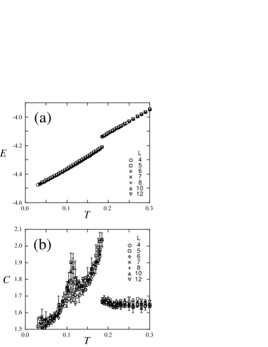
Figure 5: (a) The internal energy per site [Eq. (17)] and (b) the specific heat per site [Eq. (18)] at $J_{3}/J=0.02$. Error bars are smaller than symbol sizes in (a). Typical error bars are shown in (b).

It is noted that the specific heat approaches $3/2$ (in units of $k_{\rm B}$) as $T\rightarrow 0$ as shown in Fig. 5 (b). A finite value of $C$ at $T=0$ is characteristic to classical models, and one degree of freedom remaining at the ground state contributes $1/2$ to $C$. Hence, the data in Fig. 5 (b) suggests that there remain three degrees of freedom at $T=0$ in the present model. From the discussions of the ordered phase at low temperatures in the following sections, they can be ascribed to two transverse modes of the AF spin order and one JT mode.

From the jump of the internal energy in Fig. 5 (a), we estimate the entropy jump $\Delta{\cal S}$ associated with the first-order transition from the disordered phase above $T_{\rm O}$ to the ordered phase below $T_{\rm O}$. The two phases have the same free energy $F=E-T{\cal S}$ at $T_{\rm O}$, which gives us the entropy difference $\Delta{\cal S}$ as

$$\Delta{\cal S}=\lim_{\delta\rightarrow 0}\frac{E(T_{\rm O}+\delta)-E(T_{\rm O}-\delta)}{T_{\rm O}}\sim 0.4.$$ (19)

This corresponds to $\sim 30$-$40$% of $\ln 3$ per site.

The amount of the entropy which is related to the fluctuation around the second-order transition at $T_{\rm N}$ is estimated from the area of the anomalous peak at $T_{\rm N}$ in the plot of $C/T$ as a function of $T$. Although it is difficult to estimate it because of the large system-size dependence of $C$ as well as the large error bars in Fig. 5 (b), a rough estimate is obtained by an interpolation with polynomial functions for the normal contribution and a numerical integration of the anomalous part. The estimate is roughly $0.05$-$0.1$, which corresponds to $\sim 5$-$10$% of $\ln 3$ per site.

In experiments, the amounts of entropy related to the two transitions are also estimated from the specific heat. In ZnV₂O₄, the entropy change in the higher-temperature transition at $T_{\rm c1}$ is $\sim 3$-$4$J/mol K, i.e., $\sim 20$% of $\ln 3$ per V cation. Kondo2000 The entropy related to the lower-temperature transition at $T_{\rm c2}$ is small and not estimated quantitatively, but roughly less than $1$J/mol K, i.e., $\mathrel{\mathchoice{\lower 2.5pt\vbox{\halign{$\m@th\displaystyle\hfil#\hfil$\cr<\crcr\sim\crcr}}}{\lower 2.5pt\vbox{\halign{$\m@th\textstyle\hfil#\hfil$\cr<\crcr\sim\crcr}}}{\lower 2.5pt\vbox{\halign{$\m@th\scriptstyle\hfil#\hfil$\cr<\crcr\sim\crcr}}}{\lower 2.5pt\vbox{\halign{$\m@th\scriptscriptstyle\hfil#\hfil$\cr<\crcr\sim\crcr}}}}5$% of $\ln 3$ per V cation. Kondo2000 In MgV₂O₄, the former is estimated as $\sim 3$J/mol K, i.e., $\sim 16$% of $\ln 3$, and the latter is $\sim 0.4$J/mol K, i.e., $\sim 2$% of $\ln 3$ per V cation. Mamiya1997 Our estimates from the MC results in Fig. 5 show semiquantitative agreement with these experimental values, and particularly, explain that the entropy related to the lower-temperature transition is considerably smaller than that for the higher-temperature transition. The small entropy related to the transition at $T_{\rm N}$ is likely due to the magnetic frustration and a 1D AF correlation well developed above $T_{\rm N}$ which will be discussed in Sec. III.2.

III.1.2 High-temperature transition: Orbital ordering

To characterize two transitions in Fig. 5, we calculate corresponding order parameters. First, we consider the transition at the higher temperature $T_{\rm O}\simeq 0.19J$. Figure 6 (a) shows the sublattice orbital moment, which is defined in the form

$$M_{\rm O}=\frac{4}{N_{\rm site}}\Big{\langle}\Big{|}\sum_{i\in{\rm sublattice}}\mbox{\boldmath$I$}_{i}\Big{|}\Big{\rangle},$$ (20)

where the summation is taken over the sites within one of the four sublattices in Fig. 4 (b). Here, $\mbox{\boldmath$I$}_{i}$ is the three-state clock vector at the site $i$ which describes three different orbital states as shown in the inset of Fig. 6 (a); $\mbox{\boldmath$I$}_{i}=(1,0)$ for ($xy,yz$), $\mbox{\boldmath$I$}_{i}=(-1/2,\sqrt{3}/2)$ for ($yz,zx$), and $\mbox{\boldmath$I$}_{i}=(-1/2,-\sqrt{3}/2)$ for ($zx,xy$) orbital occupations, respectively. It is found that the values of $M_{\rm O}$ for four different sublattices have the same value within the error bars so that we omit the sublattice index in Eq. (20). As shown in Fig. 6 (a), $M_{\rm O}$ shows a clear jump at the same temperature as for the internal energy and the specific heat. This suggests that a four-sublattice orbital ordering occurs at $T_{\rm O}$. At low temperatures, $M_{\rm O}$ approaches its maximum value $1$, which indicates the four-sublattice orbital order becomes almost perfect there.

Figures 6 (b)-(e) show the orbital distribution for four sublattices $1$-$4$ shown in Fig. 4 (b), respectively, which is defined as

$$\bar{n}_{\alpha}=\frac{4}{N_{\rm site}}\sum_{i\in{\rm sublattice}}\langle n_{i\alpha}\rangle,$$ (21)

where $\alpha=1$ ($d_{yz}$), $2$ ($d_{zx}$), and $3$ ($d_{xy}$). The results indicate that at $T_{\rm O}$ the orbital distributions suddenly change from equally distributed $\bar{n}_{\alpha}\sim 2/3$ in the para phase above $T_{\rm O}$ to almost polarized $\bar{n}_{\alpha}\sim 0$ or $1$ for $T<T_{\rm O}$. In the orbital ordered phase below $T_{\rm O}$, $d_{yz}$ ($\alpha=1$) and $d_{xy}$ ($\alpha=3$) orbitals are occupied in the sublattices 1 and 4, and $d_{zx}$ ($\alpha=2$) and $d_{xy}$ ($\alpha=3$) orbitals are occupied in the sublattices 2 and 3 (Ref. note3, ). This orbital ordering structure is shown in Fig. 7. This pattern is consistent with the mean-field prediction in Fig. 4 (b).

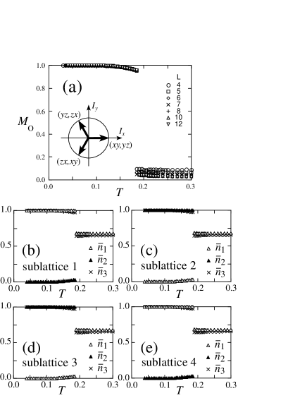
Figure 6: (a) The sublattice orbital moment in Eq. (20) at $J_{3}/J=0.02$. The inset shows the three-state clock vector for the orbital state. (b)-(d) Electron density in each orbital for four sublattices $1$-$4$ shown in Fig. 4 (b) for $L=12$ [Eq. (21)]. Error bars are smaller than the symbol sizes.

Figure 7: Orbital ordering structure obtained by MC calculations. Dark blue and light yellow octahedra in (a) contain V cations where ($d_{xy},d_{zx}$) and ($d_{xy},d_{yz}$) orbitals are occupied, respectively. They stack alternatively in the $z$ direction. Some of $d_{zx}$ and $d_{yz}$ orbitals are shown by white and black lobes, respectively. (b) is the projection of (a) from the $z$ direction. $d_{xy}$ orbitals are singly occupied at all the sites and not shown in the figures.

Accompanying the transition at $T_{\rm O}$, a tetragonal JT distortion occurs discontinuously. In Fig. 8, we plot the average of the JT distortions which is calculated by

$$\bar{Q}=\sum_{i}\langle Q_{i}\rangle/N_{\rm site}.$$ (22)

The positive value of $\bar{Q}$ below $T_{\rm O}$ corresponds to a ferro-type tetragonal JT distortion with a flattening of VO₆ octahedra as mentioned in Sec. II.1. Therefore, the level splitting shown in Fig. 4 (a) is realized. The value of $\bar{Q}$ approaches 2 at low temperatures which is the mean-field value obtained in Appendix A. We note that $\bar{Q}$ is small but finite even for $T>T_{\rm O}$. This is because $H_{\rm JT}$ breaks the cubic symmetry of the system as mentioned before.

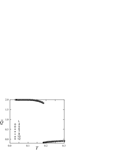
Figure 8: The average of the JT distortion defined in Eq. (22) at $J_{3}/J=0.02$. Error bars are smaller than the symbol sizes.

Therefore, the discontinuous phase transition at $T_{\rm O}$ is ascribed to the orbital ordering with the pattern of Fig. 7 accompanied by the tetragonal JT distortion with the flattening of VO₆ octahedra. From Figs. 6 and 8, we estimate $T_{\rm O}=(0.19\pm 0.01)J$ for $J_{3}/J=0.02$.

III.1.3 Low-temperature transition: Antiferromagnetic Spin Ordering

Next, we consider the other transition at $T_{\rm N}\simeq 0.115J$. Figure 9 (a) shows the temperature dependence of the staggered magnetization defined in the form

$$M_{\rm S}=\langle|\mbox{\boldmath$f$}|^{2}\rangle^{1/2},$$ (23)

where the structure factor is given by

$$\mbox{\boldmath$f$}=\frac{2}{N_{\rm site}}\sum_{i_{\rm ch}=1}^{N_{\rm ch}}\exp(2\pi il_{i_{\rm ch}}^{z})\big{[}{\sum_{i}}^{\prime}\mbox{\boldmath$S$}_{i}(-1)^{4y_{i}}\big{]}.$$ (24)

This definition looks complicated but nothing but the order parameter of the spin ordering pattern shown in Fig. 2. Here, the first summation is taken over different chains lying in the $xy$ planes ($N_{\rm ch}$ is the total number of the $xy$ chains in the system, i.e., $N_{\rm ch}=4L^{2}$ where $L$ is the linear dimension of the system measured in the cubic units), and the second summation $\sum^{\prime}$ is taken over the sites in the $i_{\rm ch}$-th $xy$ chain. $y_{i}$ is the $y$ coordinates of the site $i$, and $l_{i_{\rm ch}}^{z}$ is the $z$ coordinate of the $i_{\rm ch}$-th $xy$ chain measured in the cubic units. We set the normalization in Eq. (24) such that $M_{\rm S}$ becomes $1$ for the fully saturated AF order in Fig. 2. Note that the structure factor $f$ cannot be defined only by a real phase factor because of the complicated AF ordering pattern which is expected to have the four-period structure in the $yz$ and $zx$ directions as shown in Fig. 2. See also the discussions in Sec. III.1.4. The structure factor is also expressed in a simpler form as

$$\mbox{\boldmath$f$}=\frac{2}{N_{\rm site}}\sum_{i}g_{i}\mbox{\boldmath$S$}_{i},$$ (25)

where the form factor $g_{i}$ is given by

$$g_{i}=\cos[2\pi(x_{i}+y_{i})]+i\cos[2\pi(x_{i}-y_{i})].$$ (26)

Note that $g_{i}$ is specified only by the $x$ and $y$ coordinates of the site $i$ because the $z$ coordinate is uniquely determined within the cubic unit cell due to the special structure of the pyrochlore lattice. [See the projection in Fig. 2 (b).]

As shown in Fig. 9 (a), the staggered magnetization $M_{\rm S}$ develops continuously below $T_{\rm N}\simeq 0.115J$, and approaches the fully saturated value $M_{\rm S}=1$ as $T\rightarrow 0$. Figure 9 (b) shows the staggered magnetic susceptibility obtained by

$$\chi_{\rm S}=\frac{N_{\rm site}}{T}\big{(}\langle|\mbox{\boldmath$f$}|^{2}\rangle-|\langle\mbox{\boldmath$f$}\rangle|^{2}\big{)}.$$ (27)

Here, we calculate the susceptibility by using $\langle|\mbox{\boldmath$f$}|\rangle$ instead of $|\langle\mbox{\boldmath$f$}\rangle|$ in Eq. (27) for convenience of numerical calculations since both quantities agree with each other in the thermodynamic limit. The susceptibility $\chi_{\rm S}$ shows a diverging behavior at $T_{\rm N}$ and the peak value increases with the system size. In Fig. 9 (c), we show the Binder parameter for the staggered magnetization which is defined as Binder1981

$$g_{\rm S}=1-\frac{\langle(|\mbox{\boldmath$f$}|^{2})^{2}\rangle}{3\langle|\mbox{\boldmath$f$}|^{2}\rangle^{2}}.$$ (28)

It is known that the Binder parameter becomes larger (smaller) for larger system sizes in the ordered (disordered) phase, and hence, the crossing point of the Binder parameter for different system sizes gives a good estimate of the transition temperature. The MC data in Fig. 9 (c) shows the crossing at the same temperature of the divergence of $\chi_{\rm S}$ in Fig. 9 (b), which indicates the phase transition by the order parameter $M_{\rm S}$ at $T_{\rm N}$.

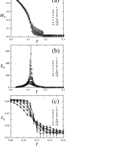
Figure 9: (a) The staggered moment defined in Eq. (23). Error bars are smaller than the symbol sizes. (b) The staggered magnetic susceptibility in Eq. (27). (c) The Binder parameter defined in Eq. (28). The lines are guides for the eyes. All the results are calculated at $J_{3}/J=0.02$.

All these results in Fig. 9 indicate that the phase transition at $T_{\rm N}$ is caused by the continuous growth of the staggered magnetic order. From Figs. 9 (b) and (c), we estimate $T_{\rm N}=(0.115\pm 0.005)J$ for $J_{3}/J=0.02$. The magnetic ordering pattern will be discussed in the next section.

III.1.4 Collinearity of magnetic ordering

The mean-field argument in Ref. Tsunetsugu2003, and in Sec. II.1 predicts that the staggered magnetizations develop independently on two sublattices and the relative angle between two AF moments is free. The two sublattices are shown in Fig. 10; one consists of the $[110]$ chains and the other consists of the $[1\bar{1}0]$ chains. The staggered magnetization $M_{\rm S}$ defined in Eq. (23) is the order parameter of the 3D AF spin ordering in Fig. 2, but cannot measure the collinearity between two staggered magnetizations. For example, $M_{\rm S}$ takes the value of $1$ independent of the relative angle between staggered moments in two sublattices, $\mbox{\boldmath$M$}_{1}$ and $\mbox{\boldmath$M$}_{2}$, shown in Fig. 10, when both sublattice moments saturate. The spin configuration in Fig. 10 is a noncollinear one, while that in Fig. 2 is a collinear one, and both give $M_{\rm S}=1$.

Here, we measure the collinearity between the staggered moments in the two sublattices by

$$C_{12}=\Big{\langle}\frac{(\mbox{\boldmath$M$}_{1}\cdot\mbox{\boldmath$M$}_{2})^{2}}{(\mbox{\boldmath$M$}_{1})^{2}(\mbox{\boldmath$M$}_{2})^{2}}\Big{\rangle}=\langle\cos^{2}\theta_{12}\rangle.$$ (29)

Here we may consider $\theta_{12}$ the angle between $\mbox{\boldmath$M$}_{1}$ and $\mbox{\boldmath$M$}_{2}$. In the present calculations, the two sublattice moments are obtained by the real and imaginary parts of the structure factor $f$ in Eq. (24) as

$$\mbox{\boldmath$M$}_{1}=\mbox{Re}(\mbox{\boldmath$f$}),\ \mbox{\boldmath$M$}_{2}=\mbox{Im}(\mbox{\boldmath$f$}),$$ (30)

respectively. If the AF order is collinear, i.e., $\mbox{\boldmath$M$}_{1}\parallel\mbox{\boldmath$M$}_{2}$, the value of $C_{12}$ become $1$. Figure 11 shows the MC results. Below $T_{\rm N}\simeq 0.115J$, $C_{12}$ is rapidly enhanced, and becomes larger and approaches $1$ as the system size increases. This indicates that the magnetic state is collinear below $T_{\rm N}$. Thus, the AF order below $T_{\rm N}$ is identified by the collinear AF spin order whose pattern is given by Fig. 2.

Figure 10: Two sublattices; one consists of the [$110$] chains (blue dashed lines) and the other consists of the [$1\bar{1}0$] chains (red solid lines). In each sublattice, chains are connected by the third-neighbor exchange $J_{3}$ in the $yz$ and $zx$ directions. Black (white) arrows show spins in the sublattice moment $\mbox{\boldmath$M$}_{1}$ ($\mbox{\boldmath$M$}_{2}$).

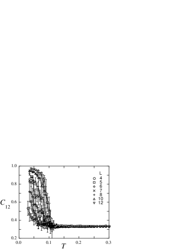
Figure 11: The collinearity defined in Eq. (29) at $J_{3}/J=0.02$. The lines are guides for the eyes.

The result indicates that thermal fluctuations in the classical version of the model (1) lift the degeneracy of the relative angle between two sublattice magnetizations and stabilize the collinear spin structure. This is a kind of the so-called order-by-disorder phenomena. Villain1977 In Sec. II.1 and Ref. Tsunetsugu2003, , we discussed that the collinear order may appear also by quantum fluctuations. Thus, we can conclude that both thermal and quantum fluctuations favor a collinear state of the two sublattice magnetizations. It is known that in many frustrated systems, thermal and quantum fluctuations favor a collinear state. This is also the case for the model (1).

III.1.5 Uniform magnetic susceptibility

We show in Fig. 12 the temperature dependence of the uniform magnetic susceptibility calculated by

$$\chi=\frac{N_{\rm site}}{T}(\langle M_{\rm tot}^{2}\rangle-\langle M_{\rm tot}\rangle^{2}),$$ (31)

where $M_{\rm tot}$ is the total magnetic moment per site, $M_{\rm tot}=|\sum_{i}\mbox{\boldmath$S$}_{i}|/N_{\rm site}.$ The result corresponds to the zero-field-cool (ZFC) result in experiments rather than the field-cool (FC) result since the susceptibility is measured by starting the MC simulation from an initial state with zero magnetic field at each temperature as described in Sec. II.3. The MC results show a sudden drop at $T_{\rm O}\simeq 0.19J$ and a little continuous change at $T_{\rm N}\simeq 0.115J$. These features qualitatively agree with the experimental results. Ueda1997

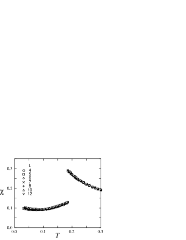
Figure 12: The uniform magnetic susceptibility in Eq. (31) at $J_{3}/J=0.02$. Error bars are smaller than the symbol sizes.

In experiments, a large difference between ZFC and FC results has been found. The difference develops from well above $T_{\rm c1}$, and remains substantial even below $T_{\rm c2}$. We will comment on this behavior in Sec. IV.4.

III.2 One-dimensional spin correlation in the intermediate phase

As shown in Fig. 9 (a), $M_{\rm S}$ in finite-size systems are enhanced below $T_{\rm O}$ even above $T_{\rm N}$. In this section, we show that there the short-range AF correlation is much enhanced along 1D chains in the $xy$ planes compared to the $yz$ and $zx$ chains.

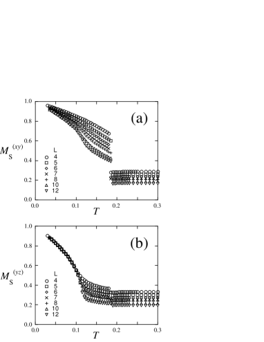
Figure 13: The staggered magnetic moment along (a) the $xy$ chains [Eq. (32)] and (b) the $yz$ chains [Eq. (33)] at $J_{3}/J=0.02$. Error bars are smaller than the symbol sizes.

The mean-field arguments in Sec. II.1 and in Ref. Tsunetsugu2003, suggest that the orbital order enhances 1D AF correlations within the $xy$ chains in the intermediate phase $T_{\rm N}<T<T_{\rm O}$. To examine the spatially anisotropic spin correlation, we calculate the staggered magnetic moments along the chains in different directions. The staggered moment along the $xy$ chains may be defined by

$$M_{\rm S}^{(xy)}=\Big{\langle}\Big{[}\frac{1}{N_{\rm ch}}\sum_{i_{\rm ch}=1}^{N_{\rm ch}}\big{|}\frac{1}{4L}{\sum_{i}}^{\prime}\mbox{\boldmath$S$}_{i}\exp(4\pi ix_{i})\big{|}^{2}\Big{]}^{1/2}\Big{\rangle},$$ (32)

where the summations are taken in the same manner as in Eq. (24), and the phase factor describes the $\uparrow$-$\downarrow$-$\uparrow$-$\downarrow$- $\cdot\cdot\cdot$ structure in the $xy$ chains as shown in Fig. 2. Similarly, the “staggered” moment along the $yz$ chains is calculated by

$$M_{\rm S}^{(yz)}=\Big{\langle}\Big{[}\frac{2}{N_{\rm ch}}\sum_{i_{\rm ch}=1}^{N_{\rm ch}}\big{|}\frac{1}{4L}{\sum_{i}}^{\prime}\mbox{\boldmath$S$}_{i}\exp(2\pi iz_{i})\big{|}^{2}\Big{]}^{1/2}\Big{\rangle},$$ (33)

where the first summation is taken over all the $yz$ chains in the system and the second summation is taken over the sites within the $i_{\rm ch}$-th $yz$ chain with a phase factor of period four in the $z$ direction with considering the $\uparrow$-$\uparrow$-$\downarrow$-$\downarrow$- $\cdot\cdot\cdot$ structure as shown in Fig. 2. Here, $N_{\rm ch}$ is the number of the $xy$ or $yz$ chains, i.e., $N_{\rm ch}=4L^{2}$ where $L$ is the linear dimension of the system measured in the unit cell. The normalization factors in Eqs. (32) and (33) are given such that both $M_{\rm S}^{(xy)}$ and $M_{\rm S}^{(yz)}$ become $1$ in the fully saturated AF state with $|\mbox{\boldmath$M$}_{1}|=|\mbox{\boldmath$M$}_{2}|=1$ in Eq. (30).

Figure 13 shows the MC results. The moment in the $zx$ chains, $M_{\rm S}^{(zx)}$, has the same value as $M_{\rm S}^{(yz)}$ within the statistical error bars. Below $T_{\rm O}\simeq 0.19J$, the moment in the $xy$ chains, $M_{\rm S}^{(xy)}$, is much more enhanced compared to that in the $yz$ and $zx$ chains, $M_{\rm S}^{(yz)}$ and $M_{\rm S}^{(zx)}$. This indicates that in the intermediate phase $T_{\rm N}<T<T_{\rm O}$, the AF spin correlations develop mainly within the $xy$ chains.

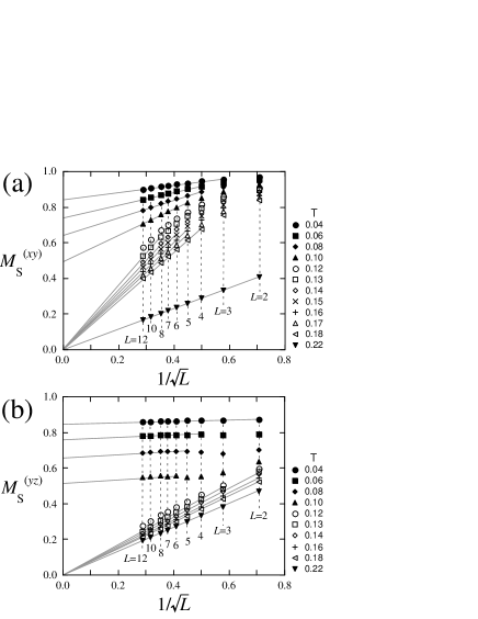
Figure 14: System-size extrapolations of the staggered magnetic moment along (a) the $xy$ chains and (b) the $yz$ chains at $J_{3}/J=0.02$. Error bars are smaller than the symbol sizes. The gray lines are the fits to a linear function of $1/\sqrt{L}$. See the text for details.

The system-size dependence of these moments within the chains provides further information. Figure 14 plots the system-size extrapolations of the MC data in Fig. 13. In the ordered phase below $T_{\rm N}\simeq 0.115J$, the MC data are extrapolated to finite values, which indicates a long-range order. The extrapolated values of $M_{\rm S}^{(xy)}$ and $M_{\rm S}^{(yz)}$ to $L\to\infty$ agree with each other within the error bars as expected in this 3D ordered phase. On the other hand, in the disordered phase above $T_{\rm O}\simeq 0.19J$, the MC data for both $M_{\rm S}^{(xy)}$ and $M_{\rm S}^{(yz)}$ well scale to $1/\sqrt{L}$ and are extrapolated to zero. (Only the data at $T=0.22J$ are shown in the figures as a typical example but other data at $T>T_{\rm O}$ show a similar behavior.) This scaling implies the exponential decay of the spin-spin correlation along the chain as explained below. Compared to the rather isotropic behavior for $T<T_{\rm N}$ and $T>T_{\rm O}$, we find a contrasting behavior between $M_{\rm S}^{(xy)}$ and $M_{\rm S}^{(yz)}$ in the intermediate phase $T_{\rm N}<T<T_{\rm O}$; almost all the data of $M_{\rm S}^{(yz)}$ well scale to $1/\sqrt{L}$ even for the smallest system size in the present calculations with $L=2$, while the data of $M_{\rm S}^{(xy)}$ show a clear deviation from the scaling in the small-$L$ region.

In order to analyze this contrasting behavior in the intermediate phase, we introduce the correlation length $\xi$ along the chain, and assume a simple scaling form of the spin-spin correlation function; the amplitude of staggered spin-spin correlation becomes an almost constant value within the length scale $\xi$ and decays exponentially for further distance than $\xi$, that is,

$$|\langle\mbox{\boldmath$S$}_{i}\cdot\mbox{\boldmath$S$}_{j}\rangle| \sim c\quad{\rm for}\ \ r_{ij}<\xi$$ (34)

$$\sim c\exp[-(r_{ij}-\xi)/\xi]\quad{\rm for}\ \ r_{ij}>\xi,$$

where $c$ is a constant and $r_{ij}=|\mbox{\boldmath$r$}_{i}-\mbox{\boldmath$r$}_{j}|$ is the distance between sites $i$ and $j$ along the chain measured in the cubic units. The staggered moments in Eqs. (32) and (33) can be rewritten by using the spin-spin correlation. For instance, Eq. (32) is rewritten in the form

$$M_{\rm S}^{(xy)} \sim \Bigg{[}\frac{1}{(4L)^{2}}{\sum_{ij}}^{\prime}\langle\mbox{\boldmath$S$}_{i}\cdot\mbox{\boldmath$S$}_{j}\cos 4\pi(x_{i}+y_{i})\rangle\Bigg{]}^{1/2}$$ (35)

$$\sim \Bigg{[}\frac{1}{\sqrt{2}L}\int\big{|}\langle\mbox{\boldmath$S$}_{0}\cdot\mbox{\boldmath$S$}_{r}\rangle\big{|}dr\Bigg{]}^{1/2},$$

by introducing the continuum limit to evaluate the summation. Note that $\sqrt{2}L$ is the length of the chains in the $L^{3}$ system. Therefore, by assuming the scaling form in Eq. (34), we obtain

$$M_{\rm S}^{(xy)}\sim\Bigg{[}\frac{1}{\sqrt{2}L}\int_{0}^{\sqrt{2}L}c\ dr\Bigg{]}^{1/2}=\sqrt{c}$$ (36)

for the case of $\xi>\sqrt{2}L$, and

$$M_{\rm S}^{(xy)} \sim \Bigg{[}\frac{1}{\sqrt{2}L}\Big{\{}\int_{0}^{\xi}c\ dr+ce\int_{\xi}^{\sqrt{2}L}\exp\big{(}-\frac{r}{\xi}\big{)}dr\Big{\}}\Bigg{]}^{1/2}$$ (37)

$$= \Bigg{[}\frac{1}{\sqrt{2}L}\Big{\{}2c\xi-ce\xi\exp\big{(}-\frac{\sqrt{2}L}{\xi}\big{)}\Big{\}}\Bigg{]}^{1/2}$$

$$\sim \frac{2^{1/4}\sqrt{c\xi}}{\sqrt{L}}$$

for the case of $\xi<\sqrt{2}L$. The staggered moment in the $yz$ chains in Eq. (33) is also estimated in a similar manner.

With considering the above arguments based on the scaling form (34), we can roughly estimate $\xi$ from the crossover of the scaling from $1/\sqrt{L}$ [Eq. (37)] to the constant [Eq. (36)] (+ corrections) in the system-size dependence in Fig. 14. That is, the linear dimension of the system size where the crossover occurs gives a rough estimate of $\xi$. For instance, at $T=0.13J$, $M_{\rm S}^{(xy)}$ deviates from the scaling of $1/\sqrt{L}$ at $L\mathrel{\mathchoice{\lower 2.5pt\vbox{\halign{$\m@th\displaystyle\hfil#\hfil$\cr<\crcr\sim\crcr}}}{\lower 2.5pt\vbox{\halign{$\m@th\textstyle\hfil#\hfil$\cr<\crcr\sim\crcr}}}{\lower 2.5pt\vbox{\halign{$\m@th\scriptstyle\hfil#\hfil$\cr<\crcr\sim\crcr}}}{\lower 2.5pt\vbox{\halign{$\m@th\scriptscriptstyle\hfil#\hfil$\cr<\crcr\sim\crcr}}}}8$, on the contrary, $M_{\rm S}^{(yz)}$ obeys the scaling down to $L\sim 3$. This suggests that $\xi^{(xy)}\sim 6$ ($\sim 16$ sites) and $\xi^{(yz)}\sim 2$ ($\sim 6$ sites). [Note that the longest distance along the chain in the periodic $L^{3}$ system ($N_{\rm site}=16L^{3}$) is $L/\sqrt{2}$.] The correlation length in the $xy$ direction is about 3 times longer than in the $yz$ and $zx$ directions. We note that the crossover length systematically shifts to a longer value as decreasing temperature, which suggests divergence of $\xi$ as $T\to T_{\rm N}$. [$\xi$ is expected to diverge in all the directions with the same critical exponent although the divergence of $\xi^{(yz)}$ is not clear in Fig. 14 (b) compared to $\xi^{(xy)}$.]

Therefore, we find a 1D anisotropy of the spin correlation: The magnitude of the moment is much enhanced and the correlation length is much longer in the $xy$ chains than in the $yz$ and $zx$ chains. As predicted in the mean-field arguments, the staggered spin correlation develops dominantly in the $xy$ chains due to the cooperation of the orbital ordering and the geometrical frustration.

Recently, the neutron scattering experiment has been performed in both above and below $T_{\rm c1}$. LeePREPRINT A clear difference of the $Q$ dependence of the inelastic neutron intensity has been found between the data above and below $T_{\rm c1}$, and ascribed to the 1D spin anisotropy due to the orbital ordering. The proposed pattern of the orbital order is the same as our result in Sec. III.1.2.

III.3 Anisotropy in optical response

It has been recognized that the interplay between orbital and spin degrees of freedom often causes an anisotropic electronic state, which is observed in optical measurements. For instance, in perovskite vanadium oxides, a strong 1D nature in the 3D lattice structure has been observed in the optical measurement, Miyasaka2002 and theoretically ascribed to the anisotropic orbital exchange in the spin ordered state. Motome2003 Therefore, we expect that the 1D anisotropy found in the previous section also shows up in the optical response.

We consider the anisotropy of the optical response by calculating the spectral weight in the present spinel case. The spectral weight is the total weight of the optical conductivity defined by

$$I_{\mu}=\frac{2\hbar^{2}}{\pi e^{2}}\int_{0}^{\infty}\sigma_{\mu\mu}(\omega)d\omega,$$ (38)

where $e$ is the electron charge, $\hbar=h/2\pi$ is the Planck’s constant, $\sigma_{\mu\mu}$ is the diagonal element of the optical conductivity tensor, and $\mu=x,y,$ or $z$. Here, we consider only the optical transfer within the $3d$ $t_{2g}$ electron bands and neglect that to the other bands such as the $3d$ $e_{g}$ bands and the oxygen $p$ bands. In experiments, the integral of Eq. (38) is calculated up to an appropriate energy cutoff to extract the spectral weight from the relevant $t_{2g}$ levels. The spectral weight in Eq. (38) is generally given by the kinetic energy in the $t_{2g}$ Hubbard model (2). Maldague1977 ; Shastry1990 In the strong correlation limit, it is calculated by the spin and orbital exchange energy in the effective model (5). Motome2003 We show in the following only the results of the calculations. Details of the calculations are explained in Appendix B.

In the calculation of the spectral weight for the present model, there are three points to be noticed. One is that the original Hubbard model (2) contains not only the nearest-neighbor but also the third-neighbor hoppings. These two types of hopping contribute differently to the spectral weight. The second point is that the directions of the electron hoppings are different from the crystal axes. Electrons hop along the $xy$, $yz$, and $zx$ chains which are canted by 45 degree from two crystal axes and perpendicular to the rest one. From this, for instance, $I_{z}$ is given by the kinetic energy both in the $zx$ and $yz$ chains but not in the $xy$ chains. The third point is the crystal symmetry. Since the system shows the tetragonal lattice distortion below $T_{\rm O}$, there holds a general relation in the form

$$I_{x}=I_{y}\neq I_{z}$$ (39)

for $T<T_{\rm O}$. We note that there remains weak anisotropy of Eq. (39) even in the high-temperature phase above $T_{\rm O}$ because of the broken cubic symmetry in $H_{\rm JT}$. With taking account of these points, we can derive the following expressions

$$I_{x} = \frac{-1}{2N_{\rm site}}\sum_{\zeta=zx,xy}\Big{[}\big{\langle}(H_{\rm SO}^{\rm nn})_{\zeta}\big{\rangle}+4\big{\langle}(H_{\rm SO}^{\rm 3rd})_{\zeta}\big{\rangle}\Big{]},$$ (40)

$$I_{y} = \frac{-1}{2N_{\rm site}}\sum_{\zeta=xy,yz}\Big{[}\big{\langle}(H_{\rm SO}^{\rm nn})_{\zeta}\big{\rangle}+4\big{\langle}(H_{\rm SO}^{\rm 3rd})_{\zeta}\big{\rangle}\Big{]},$$ (41)

$$I_{z} = \frac{-1}{2N_{\rm site}}\sum_{\zeta=yz,zx}\Big{[}\big{\langle}(H_{\rm SO}^{\rm nn})_{\zeta}\big{\rangle}+4\big{\langle}(H_{\rm SO}^{\rm 3rd})_{\zeta}\big{\rangle}\Big{]},$$ (42)

where we set $e=\hbar=1$, and $(H_{\rm SO}^{\rm nn})_{\zeta}$ and $(H_{\rm SO}^{\rm 3rd})_{\zeta}$ represent the matrix elements of Eqs. (6) and (7) in the $\zeta$ chains, respectively ($\zeta=yz$, $zx$, or $xy$). The derivation of Eqs. (40)-(42) will be given in Appendix B.

In Fig. 15, we show the MC results for the spectral weight. The spectral weight becomes highly anisotropic in the tetragonal phase below $T_{\rm O}$ with satisfying the relation (39): The spectral weight in the $z$ direction, $I_{z}$, is suddenly suppressed at $T_{\rm O}$, while those in the $xy$ plane, $I_{x}$ and $I_{y}$, are slightly enhanced there. Moreover, in the orbital ordered phase below $T_{\rm O}$, $I_{x}$ and $I_{y}$ increase monotonically with decreasing temperature, whereas $I_{z}$ shows a complicated temperature dependence although the dependence itself is small; $I_{z}$ slightly decreases above $T_{\rm N}$, and it turns to increase below $T_{\rm N}$. The increase below $T_{\rm N}$ comes from the energy gain in the $yz$ and $zx$ directions by the development of the AF spin order.

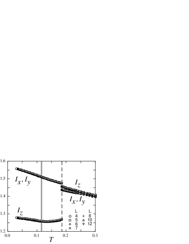
Figure 15: The spectral weights for the $x$, $y$, and $z$ direction calculated by Eqs. (40)-(42) at $J_{3}/J=0.02$. Error bars are smaller than the symbol sizes. The solid (dashed) line shows $T_{\rm N}$ ($T_{\rm O}$).

The anisotropic electronic state indicated by our MC results can be observed in the optical measurements with applying the electric field in each direction. It needs a clean surface in the single crystal. Unfortunately, it is difficult to grow a single crystal large enough thus far, and the experimental confirmation of our results remains for further study.

III.4 Systematic changes for $J_{3}/J$ and phase diagram

Here, we discuss systematic changes with respect to the value of $J_{3}/J$. Figures 16, 17, and 18 show the specific heat in Eq. (18), the uniform magnetic susceptibility in Eq. (31), and the orbital and magnetic moments in Eqs. (20) and (23), respectively, for several values of $J_{3}/J$. The orbital and JT transition temperatures $T_{\rm O}$ are indicated by the dashed lines in the figures, which are monitored by discontinuous changes of $C$, $\chi$, and $M_{\rm O}$ as well as $E$ and $\bar{Q}$ (not shown here). The AF transition temperatures $T_{\rm N}$ are indicated by the downward arrows in the figures, which are determined by the singular peak of $C$ and a continuous development of $M_{\rm S}$ as well as the diverging peak of $\chi_{\rm S}$ and the crossing point of $g_{\rm S}$ (not shown here).

In the case of $J_{3}=0$, the system shows only the orbital and lattice transition, and there is no AF ordering down to the lowest temperature. Upon switching on $J_{3}$, the magnetic transition appears at a finite temperature $T_{\rm N}$, below which the 3D AF order exists. As shown in Figs. 16-18, $T_{\rm N}$ increases whereas $T_{\rm O}$ slightly decreases as $J_{3}/J$ increases. The increase of $T_{\rm N}$ is easily understood because the AF spin ordering is stabilized by the third-neighbor exchange interaction $J_{3}$. The reason for the decrease of $T_{\rm O}$ is not so clear, but it might be due to the strong interplay between spin and orbital degrees of freedom as well as the frustration between $J$ and $J_{3}$ within the same chains. For $J_{3}/J\mathrel{\mathchoice{\lower 2.5pt\vbox{\halign{$\m@th\displaystyle\hfil#\hfil$\cr>\crcr\sim\crcr}}}{\lower 2.5pt\vbox{\halign{$\m@th\textstyle\hfil#\hfil$\cr>\crcr\sim\crcr}}}{\lower 2.5pt\vbox{\halign{$\m@th\scriptstyle\hfil#\hfil$\cr>\crcr\sim\crcr}}}{\lower 2.5pt\vbox{\halign{$\m@th\scriptscriptstyle\hfil#\hfil$\cr>\crcr\sim\crcr}}}}0.04$, $T_{\rm N}$ coincides with $T_{\rm O}$, and there is only one discontinuous transition where both orbital and AF spin moments become finite discontinuously.

Figure 16: Temperature dependences of the specific heat at (a) $J_{3}/J=0.0$, (b) $0.01$, (c) $0.02$, (d) $0.03$, (e) $0.04$, and (f) $0.05$, respectively. The dashed lines (the downward arrows) indicate $T_{\rm O}$ ($T_{\rm N}$). Typical error bars are shown.

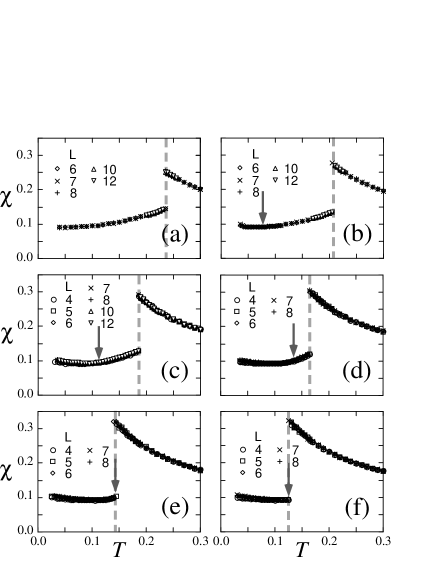
Figure 17: Temperature dependences of the uniform magnetic susceptibility at (a) $J_{3}/J=0.0$, (b) $0.01$, (c) $0.02$, (d) $0.03$, (e) $0.04$, and (f) $0.05$, respectively. The dashed lines (the downward arrows) indicate $T_{\rm O}$ ($T_{\rm N}$). Error bars are smaller than the symbol sizes.

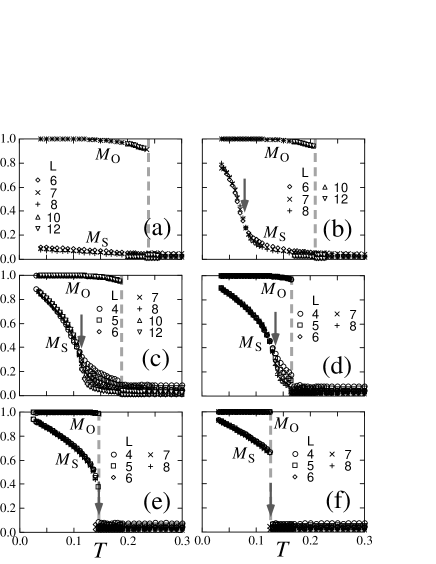
Figure 18: Temperature dependences of the orbital sublattice moment and the staggered magnetic moment at (a) $J_{3}/J=0.0$, (b) $0.01$, (c) $0.02$, (d) $0.03$, (e) $0.04$, and (f) $0.05$, respectively. The dashed lines (the downward arrows) indicate $T_{\rm O}$ ($T_{\rm N}$). Error bars are smaller than the symbol sizes.

Figure 19 summarizes the phase diagram in the $J_{3}$-$T$ parameter space determined by the analysis of the results in Figs. 16-18 as well as other quantities such as $E$, $\bar{Q}$, $\chi_{\rm S}$, and $g_{\rm S}$. The shaded area for $T_{\rm N}<T<T_{\rm O}$ shows the orbital ordered phase with the tetragonal JT distortion with a flattening of VO₆ octahedra as shown in Fig. 4 (a). The 1D anisotropy of spin correlation found in Sec. III.2 appears in this region. The hatched area for $T<T_{\rm N}$ is the AF ordered phase concomitant with the orbital and lattice orders.

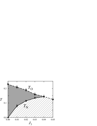
Figure 19: Phase diagram for the spin-orbital-lattice coupled model (1) determined by classical Monte Carlo calculations. The shaded area $T_{\rm N}<T<T_{\rm O}$ shows the orbital and lattice ordered phase. The hatched area below $T_{\rm N}$ is the AF ordered phase concomitant with the orbital and lattice orders. The orbital and lattice transition at $T_{\rm O}$ (the dashed line) is a first-order transition, while the AF transition at $T_{\rm N}$ (the solid line) is a second-order one. The lines are guides for the eyes.

From estimates of parameters in Sec. II.2, we obtained $J\sim 200$K and $J_{3}\sim 0.02J\sim 4$K. From Fig. 19, these estimates give $T_{\rm O}\sim 40$K and $T_{\rm N}\sim 20$K. The experimental values are $T_{\rm c1}\simeq 50$K and $T_{\rm c2}\simeq 40$K in ZnV₂O₄. Ueda1997 Thus, two transitions at $T_{\rm c1}$ and $T_{\rm c2}$ in experiments are consistently understood by the orbital and lattice ordering transition at $T_{\rm O}$ and the AF ordering transition at $T_{\rm N}$, respectively. The semiquantitative agreement of the transition temperatures between our MC results and the experimental values is satisfactory with considering the assumptions on the derivation of the model (1) and on parameter estimates in Sec. II.2. In particular, we note that $\gamma$ and $\lambda$ in the JT part in Eq. (16), are parameters in our theory for which there has not been any experimental estimate to our knowledge as mentioned in Sec. II.2. The agreement in spite of these assumptions strongly suggests that our model (1) captures essential physics in vanadium spinel oxides $A$V₂O₄.

IV Discussions

IV.1 Role of tetragonal JT distortion

The orbital and lattice orderings at $T_{\rm O}$ are considered to be caused by the cooperation between the intersite orbital interaction in Eq. (5) and the JT coupling in Eq. (16). In this section, we examine the role of the JT distortion in more detail.

We focus on the instability in the orbital sector and neglect spins momentarily. That is, we here consider the effective orbital model which is derived from the model (5) by assuming the spin paramagnetic state in the mean-field level as discussed in Ref. Tsunetsugu2003, . We replace $\mbox{\boldmath$S$}_{i}\cdot\mbox{\boldmath$S$}_{j}$ by $\langle\mbox{\boldmath$S$}_{i}\cdot\mbox{\boldmath$S$}_{j}\rangle=0$ in Eq. (5), and obtain the effective orbital Hamiltonian in the form

$$H_{\rm O}=J_{\rm O}\sum_{\langle i,j\rangle}n_{i\alpha(ij)}n_{j\alpha(ij)},$$ (43)

where $J_{\rm O}=J(2A-C)$. For simplicity, we neglect small contributions from the $J_{3}$ terms in this section. Since $J_{\rm O}>0$, the Hamiltonian is an AF three-state clock model, which is the same as Eq. (5) in Ref. Tsunetsugu2003, up to irrelevant constants.

The mean-field argument for the model (43) predicts that a degeneracy remains partially in the tetrahedron unit. Tsunetsugu2003 There are totally $3^{4}=81$ different orbital states in the four-sites unit, and $30$ states among them are in the lowest energy state which have four antiferro-type and two ferro-type orbital bonds. The $30$ degenerate states are categorized into two different types shown in Fig. 2 (a) and (b) in Ref. Tsunetsugu2003, . [The former corresponds to Fig. 4 (b) and the latter corresponds to Figs. 22 (a) and (b) in the present paper.] In the first type, two ferro-type bonds do not touch with each other, while they touch at one site in the second type. Thus, we expect that in the absence of the JT coupling, the orbital degeneracy remains partially and prevents the emergence of a particular ordered state.

To confirm this prediction, we perform the Monte Carlo simulation for the effective orbital model (43). The result of the specific heat per site is shown in Fig. 20 (a) (black symbols). The data show a broad peak around $T\simeq 0.4J_{\rm O}$ without any singularity or any significant system-size dependence. This indicates that the system does not show any phase transition, as predicted by the above mean-field picture. In Fig. 20 (b) (black symbols), we plot the temperature dependence of the entropy sum defined by

$${\cal S}(T)=\int_{0}^{T}\frac{C(T^{\prime})}{T^{\prime}}dT^{\prime}.$$ (44)

The entropy sum appears to saturate at $\sim 0.5$ at high temperatures, which is largely suppressed from the expected value of $\ln 3\simeq 1.1$ for free three-state clock spins. This indicates that there remains the entropy at zero temperature due to the degeneracy discussed above.

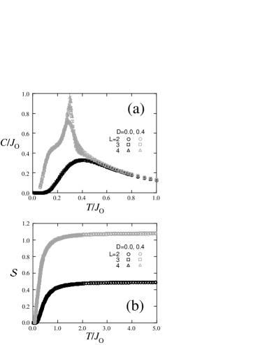
Figure 20: Temperature dependences of (a) the specific heat per site and (b) the entropy sum [Eq. (44)] for the effective orbital model (43). Black symbols show the results without the JT distortion. Gray symbols show the results in the presence of the tetragonal JT level splitting with $D/J_{\rm O}=0.4$ in Eq. (47).

One way to estimate the zero-temperature entropy ${\cal S}_{0}$ is the so-called Pauling’s method. Liebmann1986 In this method, the ground state degeneracy in the whole system is calculated simply multiplying the local degeneracy. In the present case, the total number of states is $3^{N_{\rm site}}$, and $30$ of $81$ states constitute the degenerate ground-state in each tetrahedron as mentioned above. With noting that there are $N_{\rm site}/2$ tetrahedra in the system and assuming that the tetrahedra are independent with each other, the zero-temperature entropy within the Pauling’s approximation is obtained as

$${\cal S}_{0} = \lim_{N_{\rm site}\to\infty}\frac{1}{N_{\rm site}}\ln\Big{[}3^{N_{\rm site}}\Big{(}\frac{30}{81}\Big{)}^{N_{\rm site}/2}\Big{]}$$ (45)

$$= \ln 3-\frac{1}{2}\ln\Big{(}\frac{81}{30}\Big{)}.$$

Thus, we obtain the entropy sum as

$${\cal S}(T\to\infty)=\ln 3-{\cal S}_{0}=\frac{1}{2}\ln\Big{(}\frac{81}{30}\Big{)}\simeq 0.5.$$ (46)

The estimate is close to the saturated value in Fig. 20 (b).

The tetragonal JT distortion with a flattening of the octahedra as shown in Fig. 4 (a) splits the degenerate energy levels, and lowers the energy of one orbital state of the first type, i.e., the configuration in Fig. 4 (b). In this case, all the tetrahedra are in the same orbital states. That is, there we expect the orbital ordering and disappearance of the zero-temperature entropy. The results for the case with the level splitting are also shown in Fig. 20 (gray symbols). Here, for simplicity, we incorporate the level splitting by adding the term

$$H_{D}=-\frac{D}{3}\sum_{i}(n_{i1}+n_{i2}-2n_{i3})$$ (47)

to Eq. (43), which mimics the JT term in Eq. (16). As expected, the specific heat in Fig. 20 (a) shows a singularity at $T\sim 0.3J_{\rm O}$, which indicates a phase transition. Figure 20 (b) shows ${\cal S}(T\to\infty)\simeq\ln 3$, which indicates that the phase transition reduces the remaining entropy by lifting the degeneracy.

The results in this section confirm the mean-field picture in Ref. Tsunetsugu2003, , and explicitly show the importance of the cooperation between the intersite orbital interaction and the JT coupling.

IV.2 Symmetry of orbital ordered state

Here, we comment on the spatial symmetry of the orbital ordered state below $T_{\rm O}$. Our result in Fig. 7 indicates that the orbital ordering breaks the mirror symmetry for the $[110]$ or $[1\bar{1}0]$ plane. The symmetry breaking will also appear in the lattice structure through the electron-phonon coupling which breaks the $d_{yz}$ and $d_{zx}$ symmetry although such coupling is not included in our model [the tetragonal JT mode in Eq. (16) does not split the $d_{yz}$ and $d_{zx}$ levels].

Recently, the orbital ordered state with another symmetry has been proposed theoretically. TchernyshyovPREPRINT The theory is based on the assumption of the dominant role of the relativistic spin-orbit coupling. The predicted orbital order consists of the ferro-type occupation of the $d_{xy}$ and $(d_{yz}+id_{zx})$ orbitals at every site. This orbital order does not break the mirror symmetry.

The difference of the resultant orbital ordered state is important to consider the fundamental physics of the present $t_{2g}$ electron system. In $t_{2g}$ electron systems, in general, there is keen competition among different contributions whose energy scales are close to each other; the spin and orbital exchange interactions, the JT coupling, and the relativistic spin-orbit coupling. Kugel1982 In our argument, the former two mechanisms play a primary role while the last one is not taken into account. On the contrary, in Ref. TchernyshyovPREPRINT, , the relativistic spin-orbit coupling is assumed to be dominant. Therefore, the determination of the orbital and lattice symmetry is relevant to clarify the primary factor in the keen competition.

Experimental results on the lattice symmetry, however, are still controversial. In Refs. Nishiguchi2002, and Reehuis2003, , the X-ray scattering results for polycrystal samples are consistent with the symmetry $I4_{1}/amd$ below $T_{\rm c1}$, which suggests the persistence of the mirror symmetry at the low temperature phase. On the contrary, in recent synchrotron X-ray data for a single crystal sample, a new peak is found whose intensity is three orders of magnitude weaker than a typical main peak. LeePREPRINT Unfortunately, the new peak cannot conclude whether the mirror symmetry is broken or not, but it suggests the different symmetry from the previous $I4_{1}/amd$, i.e., either $I\bar{4}m2$ or $I\bar{4}$. This controversy, probably coming from a small electron-phonon coupling in this $t_{2g}$ system, reveals the necessary of more sophisticated experiments for larger single crystals. Such experiments are highly desired to settle the theoretical controversy.

Another possible experiment to conclude the symmetry problem is to detect the orbital state directly. This may be achieved, for instance, by the resonant X-ray scattering technique. Murakami1998 Besides, another way to distinguish the orbital ordered states in our results and in Ref. TchernyshyovPREPRINT, is to examine the time reversal symmetry. The $(d_{yz}+id_{zx})$ orbital order in Ref. TchernyshyovPREPRINT, breaks the time reversal symmetry even above the magnetic transition temperature. A possible experiment is the detection of either circular dichroism or birefringence.

IV.3 Quantum fluctuation effect

Our classical Monte Carlo calculations have shown that with approaching zero temperature, the staggered moment increases and saturates at the maximum value, $M_{\rm S}\rightarrow 1$, when the third-neighbor coupling $J_{3}$ is finite. In physical units, this value should be multiplied by $gS\mu_{\rm B}$ and corresponds to $M_{\rm S}=2\mu_{\rm B}$. Here, $\mu_{\rm B}$ is the Bohr magneton and the $g$-factor is assumed to be the standard value $g=2$. This behavior was plotted in Figs. 9 (a) and 18 (b)-(f). On the other hand, recent experiments show $M_{\rm S}\sim 0.6\mu_{\rm B}$ at low temperatures, only less than a half of this classical value. LeePREPRINT ; Reehuis2003 It is well known that quantum fluctuations due to magnon excitations reduce the amplitude of spontaneous moment in antiferromagnets. We expect that this effect is particularly important in frustrated magnets like pyrochlore systems, since frustration generally reduces the energy scale of magnon excitations and correspondingly enhances quantum fluctuations of the staggered moment.

Here, we examine at $T=0$ the effect of quantum fluctuations of spin degree of freedom on the reduction of staggered moment for the model (1), by using the linear spin wave theory. For this purpose, we assume the perfect orbital order with the ordering pattern in Fig. 7, and substitute the density operators in Eq. (5) by their expectation values 0 or 1. That is, we here consider the effective quantum spin model on the pyrochlore lattice in the form

$$H_{\rm spin}=\sum_{\langle i,j\rangle}J_{ij}\mbox{\boldmath$S$}_{i}\cdot\mbox{\boldmath$S$}_{j}+{\sum_{\langle\!\langle i,j\rangle\!\rangle}}J_{3}^{\prime}\mbox{\boldmath$S$}_{i}\cdot\mbox{\boldmath$S$}_{j},$$ (48)

where the first summation should be taken over nearest-neighbor pairs, while the second one be over third-neighbor pairs coupled by $\sigma$-bond. Under the orbital ordering in Fig. 7, exchange coupling constants are ferromagnetic for nearest-neighbor spin pairs on the $yz$ and $zx$ chains, $J_{ij}=-JB=J_{\rm F}<0$, and antiferromagnetic for those on the $xy$ chains, $J_{ij}=JC=J_{\rm AF}>0$, while the third-neighbor couplings are also antiferromagnetic, $J_{3}^{\prime}=J_{3}C$. These parameters were defined in Eqs. (10)-(15). It is important that $J_{\rm AF}\gg|J_{\rm F}|\gg J_{3}^{\prime}$, since $\eta\ll 1$ and $t_{\sigma}^{\rm 3rd}\ll t_{\sigma}^{\rm nn}$. Roughly speaking, the small control parameter in the spin wave theory is 1/[$S\times z$ (number of neighbors)]. In the present case, $S$=1 and $z$=6, leading to a control parameter small enough, and therefore we may expect quite good estimate from the spin wave theory.

For the magnetic order determined by the mean field arguments in Sec. II.1 and Ref. Tsunetsugu2003, , we have calculated the reduction of staggered moment at $T=0$ by using the linear spin wave theory. The magnetic structure is shown in Fig. 2 and its unit cell contains 8 spins. Details of the calculations will be reported elsewhere and here we show only the results for the staggered moment.

When the third-neighbor exchange couplings are zero ($J_{3}^{\prime}=0$), magnons have zero energy (zero modes) on the planes $k_{x}=\pm k_{y}$ in the Brillouin zone. Within the linear spin wave theory, magnons are treated as noninteracting to each other, and these zero modes are excited freely without any energy cost. This leads to the logarithmic divergence of the reduction of moment, $\Delta S\rightarrow\infty$. It is noted that in the pyrochlore spin system in which all the nearest-neighbor couplings are antiferromagnetic with same amplitude, a half of magnon excitations are zero modes throughout the whole Brillouin zone, and this results in $\Delta S=\infty$, as a manifestation of strong geometrical frustration. Tsunetsugu2002a

Once the third-neighbor exchange couplings $J_{3}^{\prime}$ are switched on, zero modes acquire a positive energy and the reduction of moment becomes finite. Figure 21 shows the results of the reduction of moment $\Delta S$ as a function of $J_{3}^{\prime}$ for $J_{\rm AF}=1$ and $J_{\rm F}=-0.113$, corresponding to $\eta=0.08$ at which the MC calculations have been performed. The amplitude of staggered moment is reduced to $M_{\rm S}=(S-\Delta S)g\mu_{\rm B}$. In the case of the vanadium spinel oxides with $S=1$, $S-\Delta S>0$ for $J_{3}^{\prime}\mathrel{\mathchoice{\lower 2.5pt\vbox{\halign{$\m@th\displaystyle\hfil#\hfil$\cr>\crcr\sim\crcr}}}{\lower 2.5pt\vbox{\halign{$\m@th\textstyle\hfil#\hfil$\cr>\crcr\sim\crcr}}}{\lower 2.5pt\vbox{\halign{$\m@th\scriptstyle\hfil#\hfil$\cr>\crcr\sim\crcr}}}{\lower 2.5pt\vbox{\halign{$\m@th\scriptscriptstyle\hfil#\hfil$\cr>\crcr\sim\crcr}}}}10^{-3}J_{\rm AF}$, which indicates that the antiferromagnetic order shown in Fig. 2 is stable down to very small third-neighbor exchange couplings. For example, at a reasonable value, $J_{3}^{\prime}\sim 0.02J_{\rm AF}$, the amplitude of staggered moment is $M_{\rm S}\sim(1-0.5)g\mu_{\rm B}\sim 0.5g\mu_{\rm B}$. With using $g=2$, this corresponds to $M_{\rm S}\sim 1\mu_{\rm B}$. Hence, the reduction is significantly large in the present spin-orbital-lattice coupled system, and particularly the staggered moment rapidly decreases as $J_{3}^{\prime}$ in the realistic small-$J_{3}^{\prime}$ region. We consider that the estimate of $M_{\rm S}$ is satisfactory and can explain the experimental value by carefully tuning the model parameters.

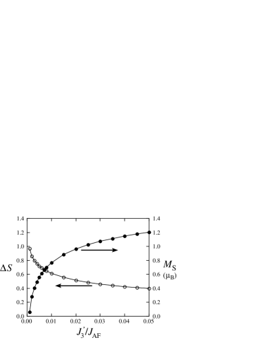
Figure 21: Reduction of the staggered moment due to quantum fluctuations (open symbols) estimated by the linear spin wave calculation at $J_{\rm F}/J_{\rm AF}=-0.113$. The staggered moment is also plotted (filled symbols), which is given by $M_{\rm S}=(S-\Delta S)g\mu_{\rm B}$ and by assuming $g=2$. The lines are guides for the eyes.

We also note that there may be a small contribution from quantum fluctuations in the orbital degree of freedom. In our spin-orbital-lattice coupled model (1), this contribution is not taken into account since we consider only $\sigma$ bond for hopping integrals. Other hopping integrals lead to small orbital exchange interactions, causing small quantum fluctuations of orbitals. This will slightly reduce the orbital sublattice moment and may lead to a further reduction of the staggered spin moment.

IV.4 Difference of ZFC and FC susceptibility

We have shown that the MC results for the uniform magnetic susceptibility in Sec. III.1.5 qualitatively explain the experimental data in the zero-field-cool (ZFC) measurement. In experiments, there has been reported that the ZFC and field-cool (FC) data show a large difference at low temperatures. Ueda1997 The difference between the ZFC and FC data emerges at a higher temperature than the structural transition temperature $T_{\rm c1}$, and develops on cooling. One of the mysteries is that the difference remains finite and large even in the AF spin ordered phase below $T_{\rm c2}$: The FC value becomes nearly twice of the ZFC one at the lowest temperature. This strongly suggests that the difference cannot be explained as a simple spin-glass phenomenon.

A key observation is that the starting temperature of the difference between the ZFC and FC data as well as the magnitude of the difference appears to depend on samples. In Ref. Ueda1997, , the difference emerges at $T\sim 100$K, and becomes $\sim 0.8\times 10^{3}$emu/V-mol at $T_{\rm c1}$. On the other hand, in Ref. Reehuis2003, , the difference starts at $T\sim 70$K, and becomes $\sim 0.3\times 10^{3}$emu/V-mol at $T_{\rm c1}$. We also note that the temperature dependences of the ZFC data show a sample dependence, especially near two transition temperatures. These sample dependences imply the importance of quenched disorder. Effects of disorder in the present spin-orbital-lattice coupled system are interesting and open problems.

In our MC calculations, it is difficult to obtain the FC results because the system shows a discontinuous transition at $T_{\rm O}$: There appears a huge hysteresis when we change the temperature successively by using the MC sample in the previous run as the initial state in the next run. On cooling, the system remains in the high-temperature para state well below the true transition temperature $T_{\rm O}$ as a metastable state because of an exponentially large energy barrier in the first-order transition. One way to avoid this hysteresis is to apply more sophisticated MC method such as the multicanonical technique. Berg1991 This interesting problem is left for further study.

IV.5 $A$-site substitution effect

We have shown that our spin-orbital-lattice coupled model (1) exhibits two transitions which well agree with experimental results in $A$V₂O₄. Here, we discuss a difference among the compounds with different $A$ cations observed in experiments.

Among $A$V₂O₄ with $A$=Zn, Mg, or Cd, CdV₂O₄ shows a different behavior near $T_{\rm c1}$ from others. Nishiguchi2002 As temperature decreases, the magnetic susceptibility for the compounds with $A$=Zn and Mg shows a sudden drop at $T_{\rm c1}$ as in our numerical result in Fig. 12, whereas that for the Cd compound shows a sharp increase. Moreover, the transition temperature $T_{\rm c1}$ is substantially higher in the Cd case than in the Zn and Mg cases; $T_{\rm c1}=97$K for Cd while $T_{\rm c1}=52$K and $64.5$K for Zn and Mg, respectively. On the other hand, the AF magnetic transition temperature $T_{\rm c2}$ is almost the same among three compounds; $T_{\rm c2}=44,45$, and $35$K for Zn, Mg, and Cd, respectively. Nishiguchi2002

Our results show that the transition temperature $T_{\rm O}$, which corresponds to $T_{\rm c1}$, is determined by the energy balance between the intersite orbital interaction in Eq. (5) and the elastic energy gain in Eq. (16). The $A$-site cations are nonmagnetic and locate at the tetrahedral sites which are separated from the pyrochlore network of V cations, and the change of the $A$ cation may affect the lattice structure since $A$O₄ tetrahedra share oxygen ions with VO₆ octahedra. Thereby, we may consider that the Cd cation, which has relatively large ionic radius, may modify the lattice structure and have an influence on the JT energy gain as well as the form and magnitude of the orbital interaction.

Actually, although the symmetry is the same for the three compounds, the so-called $u$ parameter of the spinel structure is considerably larger for CdV₂O₄ than for Zn and Mg compounds. The $u$ parameter represents the magnitude of the trigonal distortion. The absence of the trigonal distortion gives $u=0.375$ by definition, and a larger $u$ denotes a larger trigonal distortion. For the Zn and Mg cases, $u=0.385$ and $0.386$, respectively, whereas $u$ becomes 0.394 for the Cd compound: The trigonal distortion is substantially larger in the Cd case than in the Zn and Mg cases. This suggests that the peculiar behavior in CdV₂O₄ may be ascribed to effects of the trigonal distortion.

The agreement between the experimental data in Zn and Mg compounds and our numerical results, which do not include effects of the trigonal distortion, indicates that the small trigonal distortion does not play an important role in these two compounds. To understand the behavior of the Cd compound, i.e., the sharp increase in the magnetic susceptibility as well as the higher $T_{\rm c1}$, it is interesting to examine the effect of the trigonal distortion in our theoretical framework. In addition to the contribution from the electron-phonon coupling to the trigonal distortion, we may have to include more complicated hopping integrals not only the $\sigma$-bond type but also, for instance, $\pi$-bond type or the second-neighbor hoppings, since the trigonal distortion affects the network of VO₆ octahedra: These additional hoppings modify the spin and orbital intersite interactions in the derived effective model in Eq. (5). The complicated effects of this trigonal distortion are left for further study.

V Summary

In the present work, we have investigated the microscopic mechanism of two transitions in vanadium spinel oxides $A$V₂O₄ with nonmagnetic divalent $A$ cations such as Zn, Mg, and Cd. We have focused on the role of the $t_{2g}$ orbital degree of freedom as well as spin in these strongly correlated electron systems on the geometrically frustrated lattice structure, i.e., the pyrochlore lattice consists of the magnetic V cations. We have derived the effective spin-orbital-lattice coupled model in the strong correlation limit from the multiorbital Hubbard model with explicitly taking account of the $t_{2g}$ orbital degeneracy. The effective model describes the interplay between orbital and spin, and reveals the contrasting form of the intersite interactions in two degrees of freedom; the Heisenberg type for the spin part and the three-state clock type for the orbital part. The anisotropy in the orbital interaction originates from the dominant role of the $\sigma$-bond hopping integrals in the edge-sharing configuration of VO₆ octahedra. The Jahn-Teller coupling with the tetragonal lattice distortion is also included. Thermodynamic properties of the effective model have been investigated by the Monte Carlo simulation, which is a classical one to avoid the negative sign problem due to the geometrical frustration. Quantum corrections are examined by the spin wave approximation. Main results are summarized in the following.

Our effective spin-orbital-lattice coupled model exhibits two transitions at low temperatures. As temperature decreases, first, the orbital ordering transition occurs assisted by the tetragonal Jahn-Teller distortion. This is a first-order transition. Successively, at a lower temperature, the antiferromagnetic spin order sets in. This transition is second order.

For realistic parameter values, our numerical results agree with experimental data semiquantitatively. The estimates of two transition temperatures are $T_{\rm O}\sim 40$K and $T_{\rm N}\sim 20$K, while the experimental values are $T_{\rm c1}\sim 50$K and $T_{\rm c2}\sim 40$K. The changes of the entropy at the transitions are comparable to the experimental values: In particular, the small change at $T_{\rm N}$ compared to the considerable change at $T_{\rm O}$ is well reproduced. The magnetic ordering structure in the low temperature phase is completely consistent with the neutron scattering results. The magnitude of the staggered moment at $T=0$ is largely reduced by quantum fluctuations, and the estimate by the spin wave theory reasonably agrees with the experimental data. The temperature dependence of the uniform magnetic susceptibility is similar to the experimental data. The agreement strongly indicates that our effective model captures the essential physics of the vanadium spinel compounds $A$V₂O₄.

Our results give an understanding of the mechanism of the two transitions in the vanadium spinel oxides. The present numerical study has confirmed the mean-field scenario in our previous publication, Tsunetsugu2003 and moreover, given more detailed and quantitative information. The first transition with orbital and lattice orderings is induced by the intersite orbital interaction which is three-state clock type and spatially anisotropic depending on both the bond direction and the orbital states in two sites. The anisotropy lifts the degeneracy due to the geometrical frustration inherent to the pyrochlore lattice. The tetragonal Jahn-Teller coupling also plays an important role to stabilize the particular orbital ordering pattern. The obtained orbital ordering structure is the antiferro type which consists of the alternative stacking of two ferro-type $ab$ planes; ($d_{xy},d_{yz}$) orbitals are occupied in one plane, and ($d_{xy},d_{zx}$) orbitals are occupied in the other. Once the orbital ordering takes place, the orbital state affects the spin exchange interactions through the spin-orbital interplay, and reduces the magnetic frustration partially. As a consequence, the antiferromagnetic spin correlation develops mainly in the one-dimensional chains in the $ab$ planes. We found typically about three-times longer correlation length in the $xy$ direction than in the $yz$ and $zx$ directions. At the second transition, these one-dimensional chains are ordered by the third-neighbor exchange interaction to form the three-dimensional antiferromagnetic spin order. It was found that thermal fluctuations stabilize the collinear state by the order-by-disorder type mechanism.

There still remain several open problems on this topic as discussed in Sec. IV; the controversy on the symmetry of the orbital ordered state, the large difference of the zero-field-cool and field-cool data of the magnetic susceptibility, and the $A$-site dependence, which is probably related to the trigonal distortion. They need further investigations from both experimental and theoretical viewpoints. Besides them, another important problem is the carrier doping effect on the Mott insulating materials, such as the Li doping in Zn_1-xLi_xV₂O₄. In experiments, it is known that the doping rapidly destroys the ordered states at $x=0$, and replaces them by a glassy state. Urano2000 Finally, at $x=1$, the system becomes metallic and shows a heavy-fermion like behavior. Kondo1997 ; Urano2000 We believe that our present results give a good starting point to study the interesting doping effects.

Appendix A

In this Appendix, we examine the conditions for $\gamma$ and $\lambda$ in the Hamiltonian (16) to stabilize the orbital order in Fig. 4 (b) accompanied by the tetragonal JT distortion with a flattening of VO₆ octahedra as shown in Fig. 4 (a) at low temperatures. We employ the mean-field type argument to discuss the instability at high temperatures as in Ref. Tsunetsugu2003, . Here, we consider only the nearest-neighbor interactions and neglect small contributions from $H_{\rm SO}^{\rm 3rd}$. With considering a spin disordered state and replacing $\mbox{\boldmath$S$}_{i}\cdot\mbox{\boldmath$S$}_{j}$ by $\langle\mbox{\boldmath$S$}_{i}\cdot\mbox{\boldmath$S$}_{j}\rangle=0$ in Eq. (1), we obtain the effective Hamiltonian for the orbital and JT parts as

$$H_{\rm O-JT}=J_{\rm O}\sum_{\langle i,j\rangle}n_{i\alpha(ij)}n_{j\alpha(ij)}+H_{\rm JT},$$ (49)

where $J_{\rm O}=J(2A-C)$. The first term is equivalent to Eq. (43) and to Eq. (5) in Ref. Tsunetsugu2003, up to irrelevant constants.

We consider the orbital state and the JT distortion in the tetrahedron unit shown in Fig. 4 (b). For an orbital configuration at the four sites, the expectation value of the JT part $H_{\rm JT}$ for one tetrahedron is written in the following quadratic form

$$e_{\rm JT}(\mbox{\boldmath$Q$})=\mbox{\boldmath$Q$}\cdot\hat{M}\mbox{\boldmath$Q$}+\mbox{\boldmath$Q$}\cdot\mbox{\boldmath$A$}+\mbox{\boldmath$A$}\cdot\mbox{\boldmath$Q$},$$ (50)

where $Q$ is a four-dimensional vector which denotes the amplitude of the JT distortion in each site as $\mbox{\boldmath$Q$}=^{t}(Q_{1},Q_{2},Q_{3},Q_{4})$, and $\hat{M}$ is the $4\times 4$ matrix whose matrix elements are given by $\hat{M}_{ij}=1/2$ for $i=j$ and $\hat{M}_{ij}=-\lambda$ for $i\neq j$. The vector $A$ describes the electron-phonon coupling part and depends on the orbital state; for instance, $\mbox{\boldmath$A$}=^{t}(-\gamma/2,-\gamma/2,-\gamma/2,-\gamma/2)$ for the orbital occupation in Fig. 4 (b). Here, we consider the physical situation in which the system does not show any spontaneous lattice distortion without the coupling to electrons of the second and third terms in Eq. (50). This is satisfied when the matrix $\hat{M}$ is positive definite. Three of the eigenvalues of $\hat{M}$ are $(1+2\lambda)/2$ and the last one is $(1-6\lambda)/2$, and therefore, by noting that we consider only positive $\lambda$ as mentioned in Sec. II.1, the condition is

$$0<\lambda<\frac{1}{6}.$$ (51)

The quadratic form of $e_{\rm JT}$ in Eq. (50) can be transformed to the following form

$$e_{\rm JT}(\mbox{\boldmath$P$})=(\mbox{\boldmath$P$}+\mbox{\boldmath$B$})\cdot(\mbox{\boldmath$P$}+\mbox{\boldmath$B$})-\mbox{\boldmath$B$}\cdot\mbox{\boldmath$B$},$$ (52)

where $\mbox{\boldmath$P$}=\hat{L}\mbox{\boldmath$Q$}$, $\mbox{\boldmath$B$}=\hat{L}^{-1}\mbox{\boldmath$A$}$, and $\hat{L}=\hat{M}^{1/2}$ is well-defined since $\hat{M}$ is a positive-definite matrix under the condition of Eq. (51). Therefore, we find that the JT energy takes its minimum value

$$e_{\rm JT}^{\rm min}=-\mbox{\boldmath$B$}\cdot\mbox{\boldmath$B$}=-\mbox{\boldmath$A$}\cdot\hat{M}^{-1}\mbox{\boldmath$A$},$$ (53)

for the amplitude of the distortions

$$\mbox{\boldmath$Q$}^{\rm min}=-\hat{M}^{-1}\mbox{\boldmath$A$}.$$ (54)

For instance, for the configuration in Fig. 4 (b), we obtain $e_{\rm JT}^{\rm min}=-2\gamma^{2}/(1-6\lambda)$ for $\mbox{\boldmath$Q$}^{\rm min}=^{t}(Q,Q,Q,Q)$ with $Q=\gamma/(1-6\lambda)$.

All the different orbital configurations with $\langle n_{i\alpha}\rangle=0$ or $1$ are classified by the energy value $e_{\rm JT}$ into five groups, which are described by the vector $A$ as

$$\mbox{\boldmath$A$}_{1} = {}^{t}(-\gamma/2,-\gamma/2,-\gamma/2,\gamma),$$ (55)

$$\mbox{\boldmath$A$}_{2} = {}^{t}(-\gamma/2,-\gamma/2,\gamma,\gamma),$$ (56)

$$\mbox{\boldmath$A$}_{3} = {}^{t}(-\gamma/2,\gamma,\gamma,\gamma),$$ (57)

$$\mbox{\boldmath$A$}_{4} = {}^{t}(\gamma,\gamma,\gamma,\gamma),$$ (58)

$$\mbox{\boldmath$A$}_{5} = {}^{t}(-\gamma/2,-\gamma/2,-\gamma/2,-\gamma/2),$$ (59)

where arbitrary permutations of components in each vector give the same energy. Typical orbital configurations are shown in Fig. 22. (The configuration for $\mbox{\boldmath$A$}_{5}$ is shown in Fig. 4 (b).)

Figure 22: Orbital ordering patterns (a), (b), (c), and (d) for the categories 1, 2, 3, and 4 specified by Eqs. (55), (56), (57), and (58), respectively. The ferro-type (antiferro-type) orbital bonds are shown by the blue solid (red dashed) lines.

On the basis of the above consideration on the JT energy, we calculate the expectation value of the Hamiltonian (49), for the five types of orbital configurations. With considering the orbital interaction energy from the first term in Eq. (49), the minimized values of the energy per tetrahedron are obtained as

$$e_{1} = 4J_{\rm O}-\frac{\gamma^{2}(7-40\lambda)}{2(1+2\lambda)(1-6\lambda)},$$ (60)

$$e_{2} = 4J_{\rm O}-\frac{\gamma^{2}(5-26\lambda)}{(1+2\lambda)(1-6\lambda)},$$ (61)

$$e_{3} = 6J_{\rm O}-\frac{\gamma^{2}(13-28\lambda)}{2(1+2\lambda)(1-6\lambda)},$$ (62)

$$e_{4} = 8J_{\rm O}-\frac{8\gamma^{2}}{1-6\lambda}.$$ (63)

$$e_{5} = 4J_{\rm O}-\frac{2\gamma^{2}}{1-6\lambda},$$ (64)

Note that there are twelve bonds per one tetrahedron.

By comparing $e_{5}$ with other four values $e_{i}$ ($i=1-4$), we obtain the stability conditions for the orbital configuration of Fig. 4 (b). First, the conditions $e_{5}<e_{1}$ and $e_{5}<e_{2}$ are satisfied when

$$\frac{1}{10}<\lambda<\frac{1}{6}.$$ (65)

In this range, the condition $e_{5}<e_{3}$ leads to

$$\gamma^{2}<\frac{4J_{\rm O}(1+2\lambda)(1-6\lambda)}{9(1-4\lambda)},$$ (66)

and the condition $e_{5}<e_{4}$ leads to

$$\gamma^{2}<2J_{\rm O}(1-6\lambda)/3.$$ (67)

The shaded area in Fig. 23 shows the parameter region where all the conditions of Eqs. (65)-(67) are satisfied. We performed several MC runs to confirm the present mean-field type analysis. In the MC calculations in Sec. III, we take $\gamma^{2}/J=0.04$ and $\lambda/J=0.15$ as a typical set in this region.

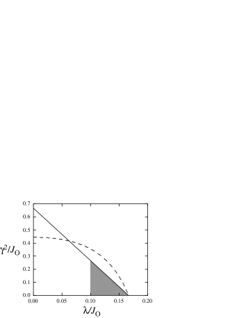
Figure 23: The parameter region of Eqs. (65)-(67) is shown by the shaded area. The dashed and solid lines denote the conditions of Eqs. (66) and (67), respectively.

Appendix B

In this appendix, we derive the expressions for the spectral weights in Eqs. (40)-(42) for our effective model (1).

The spectral weight, which is the total weight of the optical conductivity, is given by the kinetic energy of the system ($f$-sum rule). Maldague1977 ; Shastry1990 We may safely extend the formula for the single-band Hubbard model;

$$I_{\mu}=\frac{2}{\pi}\int_{0}^{\infty}\sigma_{\mu\mu}(\omega)d\omega=\frac{1}{N_{\rm u.c.}}\sum_{\mbox{\boldmath$k$}}\Big{\langle}-\frac{\partial^{2}K(\mbox{\boldmath$k$})}{\partial k_{\mu}^{2}}\Big{\rangle},$$ (68)

to our multiorbital case. (We set $e=\hbar=1$, and $N_{\rm u.c.}$ is the number of unit cells.) Here, $K(\mbox{\boldmath$k$})$ describes the kinetic energy term of the multiorbital Hubbard Hamiltonian as

$$\sum_{\mbox{\boldmath$k$}}K(\mbox{\boldmath$k$})=\sum_{\mbox{\boldmath$k$}}\sum_{a,b}\sum_{\alpha,\beta}t_{a\alpha,b\beta}(\mbox{\boldmath$k$})c_{a\alpha}^{\dagger}(\mbox{\boldmath$k$})c_{b\beta}(\mbox{\boldmath$k$}),$$ (69)

which is the Fourier transform of the first term of Eq. (2). Here, $a,b=0,1,2,3$ are the atom indices in the primitive unit-cell containing four V atoms, whose relative positions are labelled by $\mbox{\boldmath$\delta$}_{0}=(0,0,0)$, $\mbox{\boldmath$\delta$}_{1}=(0,1/4,1/4)$, $\mbox{\boldmath$\delta$}_{2}=(1/4,0,1/4)$, $\mbox{\boldmath$\delta$}_{3}=(1/4,1/4,0)$, respectively.

Since the pyrochlore lattice consists of three different chains in the $xy$, $yz$, and $zx$ directions, and we here consider only the $\sigma$-bond hopping integrals which are finite only along the chains, $K(\mbox{\boldmath$k$})$ is given by the summation of the contributions from each chain as

$$K(\mbox{\boldmath$k$})=\sum_{\zeta}\big{[}u_{\zeta}\kappa_{\zeta}^{\rm nn}(\mbox{\boldmath$k$})+v_{\zeta}\kappa_{\zeta}^{\rm 3rd}(\mbox{\boldmath$k$})\big{]},$$ (70)

where $\zeta=1$ ($yz$), $2$ ($zx$), $3$ ($xy$) denote the three different types of the chains, and $u_{\zeta},v_{\zeta}$ are the nearest-neighbor and the third-neighbor hopping integrals along the $\zeta$ chain, respectively. In the Hamiltonian (2), $u_{1}=u_{2}=u_{3}=t_{\sigma}^{\rm nn}$ and $v_{1}=v_{2}=v_{3}=t_{\sigma}^{\rm 3rd}$, but they are deliberately denoted by different parameters for later use. Each term in Eq. (70) is defined by

$$\kappa_{1}^{\rm nn}(\mbox{\boldmath$k$})=2\cos(\mbox{\boldmath$k$}\cdot\mbox{\boldmath$\delta$}_{01})[c_{01}^{\dagger}(\mbox{\boldmath$k$})c_{11}(\mbox{\boldmath$k$})+c_{11}^{\dagger}(\mbox{\boldmath$k$})c_{01}(\mbox{\boldmath$k$})]$$

$$\quad+2\cos(\mbox{\boldmath$k$}\cdot\mbox{\boldmath$\delta$}_{23})[c_{21}^{\dagger}(\mbox{\boldmath$k$})c_{31}(\mbox{\boldmath$k$})+c_{31}^{\dagger}(\mbox{\boldmath$k$})c_{21}(\mbox{\boldmath$k$})],$$ (71)

$$\kappa_{1}^{\rm 3rd}(\mbox{\boldmath$k$})=2\cos(2\mbox{\boldmath$k$}\cdot\mbox{\boldmath$\delta$}_{01})[c_{01}^{\dagger}(\mbox{\boldmath$k$})c_{01}(\mbox{\boldmath$k$})+c_{11}^{\dagger}(\mbox{\boldmath$k$})c_{11}(\mbox{\boldmath$k$})]$$

$$\quad+2\cos(2\mbox{\boldmath$k$}\cdot\mbox{\boldmath$\delta$}_{23})[c_{21}^{\dagger}(\mbox{\boldmath$k$})c_{21}(\mbox{\boldmath$k$})+c_{31}^{\dagger}(\mbox{\boldmath$k$})c_{31}(\mbox{\boldmath$k$})],$$ (72)

and so on, where $\mbox{\boldmath$\delta$}_{ab}=\mbox{\boldmath$\delta$}_{a}-\mbox{\boldmath$\delta$}_{b}$.

Let us now evaluate the derivatives of $K(\mbox{\boldmath$k$})$ in Eq. (68). By using Eq. (70), it is straightforward to obtain, for instance, the derivative in terms of $k_{x}$ in the form

$$\frac{\partial^{2}K(\mbox{\boldmath$k$})}{\partial k_{x}^{2}} = \frac{1}{16}\big{[}u_{2}\kappa_{2}^{\rm nn}(\mbox{\boldmath$k$})+u_{3}\kappa_{3}^{\rm nn}(\mbox{\boldmath$k$})\big{]}$$ (73)

$$+ \frac{1}{4}\big{[}v_{2}\kappa_{2}^{\rm 3rd}(\mbox{\boldmath$k$})+v_{3}\kappa_{3}^{\rm 3rd}(\mbox{\boldmath$k$})\big{]}.$$

The derivatives in terms of $k_{y}$ and $k_{z}$ are obtained in a similar manner. Thus, with noting $N_{\rm u.c.}=N_{\rm site}/4$, the spectral weights for the multiorbital Hubbard model (2) are obtained in the forms

$$I_{x} = -\frac{1}{4N_{\rm site}}\Big{[}\big{\{}\langle(H_{\rm K}^{\rm nn})_{zx}\rangle+\langle(H_{\rm K}^{\rm nn})_{xy}\rangle\big{\}}$$ (74)

$$\quad\quad+4\big{\{}\langle(H_{\rm K}^{\rm 3rd})_{zx}\rangle+\langle(H_{\rm K}^{\rm 3rd})_{xy}\rangle\big{\}}\Big{]},$$

$$I_{y} = -\frac{1}{4N_{\rm site}}\Big{[}\big{\{}\langle(H_{\rm K}^{\rm nn})_{xy}\rangle+\langle(H_{\rm K}^{\rm nn})_{yz}\rangle\big{\}}$$ (75)

$$\quad\quad+4\big{\{}\langle(H_{\rm K}^{\rm 3rd})_{xy}\rangle+\langle(H_{\rm K}^{\rm 3rd})_{yz}\rangle\big{\}}\Big{]},$$

$$I_{z} = -\frac{1}{4N_{\rm site}}\Big{[}\big{\{}\langle(H_{\rm K}^{\rm nn})_{yz}\rangle+\langle(H_{\rm K}^{\rm nn})_{zx}\rangle\big{\}}$$ (76)

$$\quad\quad+4\big{\{}\langle(H_{\rm K}^{\rm 3rd})_{yz}\rangle+\langle(H_{\rm K}^{\rm 3rd})_{zx}\rangle\big{\}}\Big{]},$$

where $(H_{\rm K}^{\rm nn})_{\zeta}$ and $(H_{\rm K}^{\rm 3rd})_{\zeta}$ are the nearest-neighbor and the third-neighbor matrix elements of the kinetic term in Eq. (2) along the $\zeta$ chain, respectively.

In the strong correlation limit, the kinetic energy corresponds to the spin and orbital exchange energy as discussed below. The expectation values of the kinetic terms in Eqs. (74)-(76) can be represented as coupling-constant derivatives;

$$\langle(H_{\rm K}^{\rm nn})_{\zeta}\rangle = \Big{\langle}u_{\zeta}\frac{\partial}{\partial u_{\zeta}}H_{\rm Hub}\Big{\rangle}=\frac{\partial}{\partial\ln|u_{\zeta}|}\langle H_{\rm Hub}\rangle,$$ (77)

$$\langle(H_{\rm K}^{\rm 3rd})_{\zeta}\rangle = \frac{\partial}{\partial\ln|v_{\zeta}|}\langle H_{\rm Hub}\rangle.$$ (78)

Here, we have used the Hellman-Feynman theorem to exchange the order of derivative and expectation value. In the strong correlation limit, we can replace the derivatives in terms of $u_{\zeta}$ and $v_{\zeta}$ of $\langle H_{\rm Hub}\rangle$ by the derivatives in terms of the exchange $J$ of the expectation values of the effective spin-orbital Hamiltonian (5) as

$$\frac{\partial}{\partial\ln|u_{\zeta}|}\langle H_{\rm Hub}\rangle = 2\frac{\partial}{\partial\ln|(J)_{\zeta}|}\langle H_{\rm SO}\rangle=2\langle(H_{\rm SO}^{\rm nn})_{\zeta}\rangle,$$ (79)

$$\frac{\partial}{\partial\ln|v_{\zeta}|}\langle H_{\rm Hub}\rangle = 2\frac{\partial}{\partial\ln|(J_{3})_{\zeta}|}\langle H_{\rm SO}\rangle=2\langle(H_{\rm SO}^{\rm 3rd})_{\zeta}\rangle,$$ (80)

where $(J)_{\zeta}=u_{\zeta}^{2}/U$ and $(J_{3})_{\zeta}=v_{\zeta}^{2}/U$ are the nearest-neighbor and the third-neighbor exchange coupling constants along the $\zeta$ direction, respectively; and $(H_{\rm SO}^{\rm nn})_{\zeta}$ and $(H_{\rm SO}^{\rm 3rd})_{\zeta}$ are the nearest-neighbor and the third-neighbor matrix elements of Eqs. (6) and (7) along the $\zeta$ chain, respectively. In the model (5), $(J)_{\zeta}=J=(t_{\sigma}^{\rm nn})/U$ and $(J_{3})_{\zeta}=J_{3}=(t_{\sigma}^{\rm 3rd})/U$, and they are independent of the direction $\zeta$. By substituting all the expectation values in Eqs. (74)-(76) by Eqs. (79), (80), and the similar expressions, we obtain the formulas of the spectral weights for the effective spin-orbital coupled model in the strong correlation limit as given in Eqs. (40)-(42).

References

- (1) For instance, see Magnetic System with Competing Interaction, ed. by H.T. Diep (World Scientific Publishing Co., 1994).
- (2) R. Liebmann, Statistical mechanics of periodic frustrated Ising systems (Springer-Verlag, Berlin, Tokyo, 1986).
- (3) P.W. Anderson, Phys. Rev. 102, 1008 (1956).
- (4) B. Canals and C. Lacroix, Phys. Rev. B 61, 1149 (2000).
- (5) A.B. Harris, A.J. Berlinsky, and C. Bruder, J. Appl. Phys. 69, 5200 (1991).
- (6) H. Tsunetsugu, J. Phys. Soc. Jpn. 70, 640 (2001); Phys. Rev. B 65, 024415 (2002).
- (7) A. Koga and N. Kawakami, Phys. Rev. B 63, 144432 (2001).
- (8) E. Berg, E. Altman, and A. Auerbach, Phys. Rev. Lett. 90, 147204 (2003).
- (9) J.N. Reimers, A.J. Berlinsky, and A.-C. Shi, Phys. Rev. B 43, 865 (1991); J.N. Reimers, ibid. 45, 7287 (1992).
- (10) R. Moessner and J.T. Chalker, Phys. Rev. Lett. 80, 2929 (1998); Phys. Rev. B 58, 12049 (1998).
- (11) Muhtar, F. Takagi, K. Kawakami, and N. Tsuda, J. Phys. Soc. Jpn. 57, 3119 (1988).
- (12) Y. Ueda, N. Fujiwara, and H. Yasuoka, J. Phys. Soc. Jpn. 66, 778 (1997).
- (13) S. Nizioł, Phys. Status Solidi A 18, K11 (1973).
- (14) Yu.A. Izyumov, V.E. Naish, and S.B. Petrov, J. Mag. Mag. Mater. 13, 267 (1979).
- (15) H. Mamiya, M. Onoda, T. Furubayashi, J. Tang, and I. Nakatani, J. Appl. Phys. 81, 5289 (1997).
- (16) N. Nishiguchi and M. Onoda, J. Phys: Condens. Matter 14, L551 (2002); M. Onoda and J. Hasegawa, ibid. 15, L95 (2003).
- (17) Y. Yamashita and K. Ueda, Phys. Rev. Lett. 85, 4960 (2000).
- (18) O. Tchernyshyov, R. Moessner, and S.L. Sondhi, Phys. Rev. Lett. 88, 067203 (2002); Phys. Rev. B 66, 064403 (2002).
- (19) I. Kagomiya, K. Kohn, M. Toki, Y. Hata, and E. Kita, J. Phys. Soc. Jpn. 71, 916 (2002).
- (20) M.T. Rovers, P.P. Kyriakou, H.A. Dabkowska, G.M. Luke, M.I. Larkin, and A.T. Savici, Phys. Rev. B 66, 174434 (2002).
- (21) S. Kondo, D.C. Johnston, C.A. Swenson, F. Borsa, A.V. Mahajan, L.L. Miller, T. Gu, A.I. Goldman, M.B. Maple, D.A. Gajewski, E.J. Freeman, N.R. Dilley, R.P. Dickey, J. Merrin, K. Kojima, G.M. Luke, Y.J. Uemura, O. Chmaissem, and J.D. Jorgensen, Phys. Rev. Lett 78, 3729 (1997); S. Kondo, D.C. Johnston, and L.L. Miller, Phys. Rev. B 59, 2609 (1999).
- (22) C. Urano, M. Nohara, S. Kondo, F. Sakai, H. Takagi, T. Shiraki, and T. Okubo, Phys. Rev. Lett. 85, 1052 (2000).
- (23) V.I. Anisimov, M.A. Korotin, M. Zölfl, T. Pruschke, K. Le Hur, and T.M. Rice, Phys. Rev. Lett. 83, 364 (1999).
- (24) D.J. Singh, P. Blaha, K. Schwarz, and I.I. Mazin, Phys. Rev. B 60, 16359 (1999).
- (25) I.A. Nekrasov, Z.V. Pchelkina, G. Keller, Th. Pruschke, K. Held, A. Krimmel, D. Vollhardt, and V.I. Anisimov, Phys. Rev. B 67, 085111 (2003).
- (26) V. Eyert, K.-H. Höck, S. Horn, A. Loidl, and P.S. Riseborough, Europhys. Lett. 46, 762 (1999).
- (27) J. Matsuno, A. Fujimori, and L.F. Mattheiss, Phys. Rev. B 60, 1607 (1999).
- (28) S. Fujimoto, Phys. Rev. B 64, 085102 (2001).
- (29) H. Tsunetsugu, J. Phys. Soc. Jpn. 71, 1844 (2002).
- (30) Y. Yamashita and K. Ueda, Phys. Rev. B 67, 195107 (2003).
- (31) K. Kawakami, Y. Sakai, and N. Tsuda, J. Phys. Soc. Jpn., 55, 3174 (1986).
- (32) M. Onoda, H. Imai, Y. Amako, and H. Nagasawa, Phys. Rev. B 56, 3760 (1997).
- (33) H. Tsunetsugu and Y. Motome, Phys. Rev. B 68, 060405(R) (2003).
- (34) K.I. Kugel’ and D.I. Khomskiĭ, Zh. Eksp. Teor. Fiz. 64, 1429 (1973) [Sov. Phys. JETP 37, 725 (1973)]; Fiz. Tverd. Tela, 17, 454 (1975) [Sov. Phys. Solid State 17, 285 (1975)].
- (35) We use slightly different notation for the Coulomb parameters from Ref. Tsunetsugu2003, .
- (36) Both -bond and -bond hopping integrals for second-neighbor pairs are estimated to be less than half of in Ref. Matsuno1999, .
- (37) Note that the definition of is different from that in Ref. Tsunetsugu2003, for convenience. in the present work corresponds to in Ref. Tsunetsugu2003, . Note also that Eqs. (12) and (13) are slightly modified from those in Ref. Tsunetsugu2003, because of a minor mistake in the perturbation calculation, however, these minor changes do not alter the mean-field results in Ref. Tsunetsugu2003, .
- (38) T. Mizokawa and A. Fujimori, Phys. Rev. B 54, 5368 (1996).
- (39) Y. Ozeki, K. Kasono, N. Ito, and S. Miyashita, Physica A 321, 271 (2003).
- (40) S. Kondo, C. Urano, Y. Kurihara, M. Nohara, and H. Takagi, J. Phys. Soc. Jpn. 69 Suppl. B, 139 (2000).
- (41) In the orbital ordered state below , there are two energy minima with equal energy; one is for the orbital occupations in Figs. 6 (b)-(e) and the other is for the occupations with exchanging and . In the present MC calculations, one of two configurations is selected depending on the initial configuration, and the MC sampling is performed around the selected energy minimum, since the energy barrier between the two minima is exponentially large in the first order transition.
- (42) K. Binder, Z. Phys. B 43, 119 (1981).
- (43) J. Villain, J. Phys. C: Solid State Phys. 10, 1717 (1977); Z Phys. B 33, 31 (1979).
- (44) S.-H. Lee, D. Louca, H. Ueda, S. Park, T.J. Sato, M. Isobe, Y. Ueda, S. Rosenkranz, P. Zschack, J. Íñiguez, Y. Qui, and R. Osborn, preprint (cond-mat/0312558).
- (45) S. Miyasaka, Y. Okimoto, and Y. Tokura, J. Phys. Soc. Jpn. 71, 2086 (2002).
- (46) Y. Motome, H. Seo, Z. Fang, and N. Nagaosa, Phys. Rev. Lett. 90, 146602 (2003).
- (47) P.F. Maldague, Phys. Rev. B 16, 2437 (1977).
- (48) B.S. Shastry and B. Sutherland, Phys. Rev. Lett. 65, 243 (1990); B.S. Shastry, B.I. Shraiman, R.R.P. Singh, Phys. Rev. Lett. 70, 2004 (1993).
- (49) O. Tchernyshyov, preprint (cond-mat/0401203).
- (50) K.I. Kugel’ and D.I. Khomskiĭ, Usp. Fiz. Nauk 136, 621 (1982) [Sov. Phys. Usp. 25, 231 (1982)].
- (51) M. Reehuis, A. Krimmel, N. Büttgen, A. Loidl, and A. Prokofiev, Eur. Phys. J. B 35, 311 (2003).
- (52) Y. Murakami, H. Kawada, H. Kawata, M. Tanaka, T. Arima, Y. Moritomo, and Y. Tokura, Phys. Rev. Lett. 80, 1932 (1998); Y. Murakami, J.P. Hill, D. Gibbs, M. Blume, I. Koyama, M. Tanaka, H. Kawata, T. Arima, Y. Tokura, K. Hirota, and Y. Endoh, Phys. Rev. Lett. 81, 582 (1998).
- (53) H. Tsunetsugu, J. Phys. Chem. Solids 63, 1325 (2002).
- (54) B.A. Berg and T. Neuhaus, Phys. Lett. B 267, 249 (1991); Phys. Rev. Lett. 68, 9 (1992).