Tagged-particle dynamics in a hard-sphere system: mode-coupling theory analysis

Abstract

The predictions of the mode-coupling theory of the glass transition (MCT) for the tagged-particle density-correlation functions and the mean-squared displacement curves are compared quantitatively and in detail to results from Newtonian- and Brownian-dynamics simulations of a polydisperse quasi-hard-sphere system close to the glass transition. After correcting for a 17% error in the dynamical length scale and for a smaller error in the transition density, good agreement is found over a wide range of wave numbers and up to five orders of magnitude in time. Deviations are found at the highest densities studied, and for small wave vectors and the mean-squared displacement. Possible error sources not related to MCT are discussed in detail, thereby identifying more clearly the issues arising from the MCT approximation itself. The range of applicability of MCT for the different types of short-time dynamics is established through asymptotic analyses of the relaxation curves, examining the wave-number and density-dependent characteristic parameters. Approximations made in the description of the equilibrium static structure are shown to have a remarkable effect on the predicted numerical value for the glass-transition density. Effects of small polydispersity are also investigated, and shown to be negligible.

I Introduction

Understanding the slow dynamical processes that occur when one cools or compresses a liquid is a great challenge of condensed matter physics. In particular in the time window accessible to scattering experiments or molecular-dynamics (MD) computer simulations, one observes in equilibrium a precursor of the liquid-glass transition that is commonly termed structural relaxation. From these experiments, a large amount of detailed information about the equilibrium fluctuations in such systems is available Götze (1999).

Many of the recent experiments on structural relaxation were stimulated by the mode-coupling theory of the glass transition (MCT). This theory attempts to provide a first-principles description of the slow structural relaxation processes, requiring as input the (averaged) equilibrium static structure of the system under study. Unfortunately, for many commonly studied glass formers, the latter is not available to the extent required. Thus comparisons of MCT with experiment usually proceed by referring to asymptotic predictions or schematic simplifications of the theory that can be evaluated without restriction to a specific system, and by fitting the remaining parameters of the theory. One has to be careful when interpreting these results, since it is known that most experimental data is hardly inside the regime of applicability of the asymptotic formulas Franosch et al. (1997); Götze and Th. Voigtmann (2000). Still, this way, many studies of the predicted MCT scenario have been performed (see Ref. Götze (1999) for a review).

Having established the general scenario, important questions arising are what are its ranges of validity, and what is the effect of the approximations made in the course of deriving the theory. These questions can be addressed by comparing the ‘full’ solutions of the theory to experimental results for one and the same system for which the static structure is known in detail. While work has been done along this direction to various degrees of detail recently, a coherent picture for a single prototypical system has not yet emerged. This paper aims towards filling this gap by providing a detailed comparison of computer-simulation results for a system of quasi-hard spheres with the corresponding ‘full’ MCT solutions, to establish the performance of MCT in describing the dynamics of a prototypical glass-forming system as a fully microscopic theory.

Such first-principles comparisons have become possible with the appearance of powerful MD simulations for simple model systems. Simulation data has been used to successfully test the MCT predictions for the frozen glassy structure (the long-time limit of the dynamical correlation functions) for a mixture of Lennard-Jones particles Nauroth and Kob (1997), a model silica melt Sciortino and Kob (2001), and a computer model of the molecular glass former Ortho-terphenyl Chong and Sciortino (2003). In these cases, the equilibrium-structure input to MCT was determined from the simulations themselves. The dynamical information has not been compared to MCT in these cases. This comparison has been tackled for the Lennard-Jones mixture Kob et al. (2002) and for two binary hard-sphere mixtures Foffi et al. (2004), but there the discussion had to be restricted to the slowest decay process, while qualitative deviations from MCT at intermediate and short times could not be resolved. This is in contrast to a full-MCT analysis of experimental light-scattering data from a quasi-binary hard-sphere like colloidal mixture Th. Voigtmann (2003), where agreement over the full accessible time window was found as far as MCT was concerned, including short and intermediate times. It is unclear to what extent the different system types and the different forms of short-time dynamics between the MD simulations and the colloidal system give rise to the differing results. Thus it seems appropriate to perform this comparison for an even more fundamental, paradigmatic glass former, viz.: the hard-sphere system (HSS).

Simulations for this system close to the glass transition have been performed by Doliwa and Heuer Doliwa and Heuer (1998, 2000) using a Monte Carlo procedure and a slight polydispersity. There, an emphasis was put on the analysis of cooperative motion on the single-particle level, and no quantitative connection to MCT was reported. Instead we focus on the analysis of the self-intermediate scattering functions, which can be directly compared to theory and experiment. We chose to perform molecular dynamics (MD) simulations instead of MC, in order to be able to also study the influence of different realistic types of short-time dynamics, i.e. ‘atomistic’ Newtonian dynamics (ND) and ‘colloidal’ Brownian dynamics (BD). Such a study has been performed earlier for the Lennard-Jones mixture mentioned above Gleim et al. (1998), however no full-MCT analysis was included there.

For an observation of the equilibrium glassy dynamics, it is, in general, necessary to avoid crystallization by some means. For the HSS, this can be accomplished by introducing a small amount of polydispersity that drastically reduces crystallization rates Williams et al. (2001). This is inherently the case in studies of colloidal suspensions. In the MD simulation, we are able to fully control the distribution of particle radii in the system. In colloidal suspensions, solvent-mediated hydrodynamic interactions (HI) are inevitable. It is an as yet not settled question to what extent HI influence the dynamics at high densities. In the present simulations, HI are not present. Thus our study also serves to complement previous analyses of colloidal hard-sphere suspensions with asymptotic formulas van Megen and Underwood (1993, 1994), demonstrating that HI are not an important ingredient for a quantitative description of structural relaxation.

The paper is organized as follows. First, we introduce in Sec. II the relevant quantities for the discussion. An investigation of some asymptotic properties of the simulation data is performed in Sec. III, whereas Sec. IV is devoted to a comparison of the time-dependent data with MCT results for the one-component HSS. In Sec. V, the effects of polydispersity will be discussed within the framework of this MCT analysis. We summarize our findings in the conclusions, Sec. VI.

II Simulation and Theory Details

II.1 Molecular Dynamics Simulations

We perform standard molecular-dynamics simulations of $N=1000$ particles in the canonical ensemble in a polydisperse system of quasi-hard spheres. The core-core repulsion between particles at a distance $r$ is given by

$$V_{c}(r)=k_{\text{B}}T\left(\frac{r}{d_{12}}\right)^{-36}\,,$$ (1)

where $d_{12}$ is the center-to-center distance, $d_{12}=(d_{1}+d_{2})/2$, with $d_{1}$ and $d_{2}$ the diameters of the particles. This potential is tailored to be a continuous approximation to the hard-sphere potential considered in the theoretical part of the work, as this facilitates the simulation of Brownian dynamics. The control parameters of this soft-sphere system are the number density $\varrho$ and temperature $T$; they appear however only as a single effective coupling parameter, $\Gamma=\varrho T^{-12}$ Hansen and McDonald (1986). In the simulation, $\Gamma$ is varied by changing the density and keeping the temperature fixed. In the following, we denote the number density in terms of a packing (or volume) fraction, which for a monodisperse system reads $\varphi=(\pi/6)\varrho d^{3}$. To avoid crystallization, the diameters of the particles in the simulation are distributed according to a flat distribution centered around $d$ and a half-width of $\delta/2=0.1d$. Thus the volume fraction reads $\varphi=(\pi/6)d^{3}\left[1+\delta^{2}\right]\varrho$.

Note that, due to polydispersity and finite-size effects, it is not trivial to ensure that the volume fraction remains constant among different runs, i.e. different realizations of the polydispersity distribution. If one randomly draws $N$ particles with radii according to the polydispersity distribution at a fixed number density, the resulting packing fraction will vary from run to run, by up to about $1\%$ in the cases we have investigated. This is not acceptable, since the slow dynamics to be discussed depends sensitively on the packing fraction. In order to eliminate such fluctuations of $\varphi$, we instead choose a fixed realization of the radius distribution ($1000$ equally spaced radii from $0.9$ to $1.1$), and randomly assign each radius to one of the particles in the initial configuration.

Both Newtonian and Brownian dynamics simulations were performed, to analyze the effect of the microscopic dynamics on the structural relaxation. Newtonian dynamics (ND) was simulated by integrating the Newton’s equations of motion in the canonical ensemble at constant volume. In Brownian dynamics (BD), or more precisely, strongly damped Newtonian dynamics, each particle experiences a Gaussian distributed white noise force with zero mean, $\vec{\eta}(t)$, and a damping force proportional to the velocity, $\gamma\dot{\vec{r}}$, apart from the deterministic forces from the interactions. Hence the equation of motion for particle $j$ is

$$m\ddot{\vec{r}}_{j}-\sum_{i}\vec{F}_{ij}=-\gamma\dot{\vec{r}}_{j}+\vec{\eta}_{j}(t)\,,$$ (2)

where $\gamma$ is a damping constant. The stochastic and friction forces fulfill the fluctuation-dissipation theorem, $\langle\vec{\eta}_{i}(t)\vec{\eta}_{j}(t^{\prime})\rangle=6k_{\text{B}}T\gamma\delta(t-t^{\prime})\delta_{ij}$. The value of $\gamma$ was set to $(30/\sqrt{3})\,kT/(dv_{\text{th}})$; this ‘overdamped limit’ ensures that the results presented here no longer show a dependence on the value $\gamma$. Such a form of the dynamics has been introduced in the study of glassy relaxation by Gleim et al. Gleim et al. (1998). Let us note that the short-time dynamics visible in the correlators and in the mean-squared displacement still is not strictly diffusive, but rather strongly damped ballistic. Since it is not our aim to investigate the very short-time dynamical features of the simulations, this will not be discussed in the following.

Equilibration runs were done with ND in all cases, since the damping not only introduces a change in the overall time scale but also slows down the equilibration process. Lengths are measured in units of the diameter, the unit of time is fixed setting the thermal velocity to $v_{\text{th}}=\sqrt{k_{\text{B}}T/m}=1/\sqrt{3}$, and the temperature is fixed to $k_{\text{B}}T=1/3$. In ND, the equations of motion were integrated using the velocity-Verlet algorithm Frenkel and Smit (2001), with a time step $\delta t=0.0025$. The thermostat was applied by rescaling the particle velocity to ensure constant temperature every $n_{t}$ time steps. For well equilibrated samples, no effect of $n_{t}$ was detected. The equations for Brownian motion were integrated following a Heun algorithm Paul and Yoon (1995) with a time step of $\delta t=0.0005$. In this case, no external thermostat was used, since the samples were already equilibrated when running BD simulations.

The orientational order parameter $Q_{6}$ Steinhardt et al. (1983); ten Wolde et al. (1996) was used to check that the system was not crystalline. For amorphous liquid-like structures, $Q_{6}$ is close to zero, whereas it takes a finite value for an ordered phase. Even though the $10\%$ polydispersity is high enough to prevent crystallization in most cases, some samples at the highest volume fractions studied did show a tendency to crystallize. Those have been excluded from the analysis.

The volume fractions investigated in this work are $\varphi=0.50$, $0.53$, $0.55$, $0.57$, $0.58$, $0.585$, and $0.59$. At each volume fraction, we extracted as statistical information on the slow dynamics the self part of the intermediate scattering function for several wave vectors $\vec{q}$, $\phi^{s}(q,t)=\langle\exp[-i\vec{q}(\vec{r}_{s}(t)-\vec{r}_{s}(0))]\rangle$, formed with the Fourier-transformed fluctuating density of a single ‘tagged’ particle at position $\vec{r}_{s}(t)$. Here, angular brackets $\langle\cdot\rangle$ denote canonical averaging. A related quantity which we also extracted from the simulations is the mean-squared displacement (MSD) of a tagged particle, $\delta r^{2}(t)=\langle(\vec{r}_{s}(t)-\vec{r}_{s}(0))^{2}\rangle$. The correlators and the MSD were averaged over typically $50$ runs, except for the BD simulations at $\varphi=0.585$ and $0.59$, where $20$ runs have been performed originally. For $\varphi=0.59$ we have also performed additional runs for both ND and BD in order to investigate some phenomena found there, see Sec. III.2 below.

II.2 Mode-Coupling Theory

In a system of $N$ structureless classical particles, i.e. without any internal degrees of freedom, the statistical information on the structural dynamics is encoded in the density correlation function, $\phi(q,t)=\langle\varrho(\vec{q},t)^{*}\varrho(\vec{q})\rangle$, formed with the fluctuating number densities $\varrho(\vec{q},t)=\sum_{j=1}^{N}\exp(i\vec{q}\cdot\vec{r}_{j}(t))/\sqrt{N}$ for wave vector $\vec{q}$. $\phi(q,t)$ is a real function that depends on $\vec{q}$ only through $q=|\vec{q}|$, since it is the Fourier transform of a real, translational-invariant and isotropic function. The dynamics given by $\phi(q,t)$ is probed by the mean-squared displacement, $\delta r^{2}(t)$, and the self-part of the intermediate scattering function (also called tagged-particle correlation function), $\phi^{s}(q,t)$, extracted from our simulations. Note that the latter is linked to the MSD in the limit $q\to 0$, via $\phi^{s}(q,t)=1-(1/6)q^{2}\delta r^{2}(t)+{\mathcal{O}}(q^{4})$.

The mode-coupling theory of the glass transition (MCT) Götze (1991) builds upon an exact equation of motion for the density autocorrelation function $\phi(q,t)$,

$$\frac{1}{\Omega(q)^{2}}\partial_{t}^{2}\phi(q,t)+\phi(q,t)\\ +\int_{0}^{t}m(q,t-t^{\prime})\partial_{t^{\prime}}\phi(q,t^{\prime})\,dt^{\prime}=0\,.$$ (3a)

Here, $$\Omega(q)^{2}=q^{2}v_{\text{th}}^{2}/S(q) \phi(q,t=0)=1 \partial_{t}\phi(q,t=0)=0 m(q,t) m^{\text{MCT}}(q,t)$$ is a characteristic squared frequency of the short-time motion. The equation of motion is supplemented by the initial conditions and . All many-body interaction effects are contained in the memory kernel , the description of which is the aim of the MCT approximations. One splits off from this kernel a mode-coupling contribution , while the remainder is assumed to describe regular liquid-state dynamics. Let us approximate this latter part by an instantaneous contribution,

$$m(q,t)\approx(\nu(q)/\Omega(q)^{2})\delta(t)+m^{\text{MCT}}(q,t)\,.$$ (3b)

The damping term $$\nu(q) \nu=(30/\sqrt{3})\,v_{\text{th}}/d q \phi(q,t) \phi(q,t)=1-(q^{2}/S(q))(k_{\text{B}}T/\gamma)t+{\mathcal{O}}(t^{2})=1-(\Omega(q)^{2}/\nu)t+{\mathcal{O}}(t^{2}) q \nu$$ is chosen as independent of ; a choice that ensures the short-time expansion of in the overdamped limit to match that one of the simulation, cf. Eq. (2): one gets . Note that the -independent choice of destroys momentum conservation for the hard-sphere particles; this is appropriate for a model of a colloidal system.

The MCT contribution to the memory kernel is given by $m^{\text{MCT}}(q,t)={\mathcal{F}}_{q}[\phi(t)]$, where

$${\mathcal{F}}[\hat{f}]=\frac{\varrho}{2q^{4}}\int\frac{d^{3}k}{(2\pi)^{3}}S(q)S(k)S(p)V(\vec{q},\vec{k},\vec{p})\hat{f}(k)\hat{f}(p)$$ (3c)

and the abbreviation $\vec{p}=\vec{q}-\vec{k}$ has been used. The vertices $V(\vec{q},\vec{k},\vec{p})$ are the coupling constants of the theory, through which all crucial control-parameter dependence enters. They are given entirely in terms of static two- and three-point correlation functions describing the equilibrium structure of the system’s liquid state. The latter are approximated using a convolution approximation, so that the vertex reads

$$V(\vec{q},\vec{k},\vec{p})=\left[(\vec{q}\vec{k})c(k)+(\vec{q}\vec{p})c(p)\right]^{2}\,.$$ (3d)

Here, $c(q)$ is the direct correlation function (DCF) connected to the static structure factor by $S(q)=1/(1-\varrho c(q))$.

The long-time limit of the correlation functions, $f(q)=\lim_{t\to\infty}\phi(q,t)$, is used to discriminate between liquid and glassy states. In the liquid, $f(q)\equiv 0$, while the glass is characterized by some $f(q)\neq 0$. From Eqs. (3), one finds $f(q)$ as the largest real and positive solution of the implicit equations Götze and Sjögren (1995)

$$\frac{f(q)}{1-f(q)}={\mathcal{F}}_{q}[f]\,.$$ (4)

In particular, there exist critical points in the control-parameter space, identified as ideal glass transition points, where a new permissible solution of Eq. (4) appears. Typically, $f(q)$ jumps discontinuously from zero to nonzero values there. Close to such a critical point on the liquid side, the correlation functions exhibit a two-step relaxation scenario, composed by a relaxation towards a plateau value, and by a later relaxation from this plateau value to zero termed $\alpha$ relaxation. On approaching the transition, the characteristic time scale for the $\alpha$ relaxation diverges, and an increasingly large window opens where the correlation functions stay close to their plateau. The plateau values on the liquid side are in leading order given by the critical solutions of Eq. (4), $f^{c}(q)$, i.e. by the maximal solutions of Eq. (4) evaluated at a critical point. The time window for which $\phi(q,t)$ is close to $f^{c}(q)$ is called the $\beta$-relaxation regime, and is the object of asymptotic predictions of MCT Götze (1991); Franosch et al. (1997); Fuchs et al. (1998). These include scaling laws for the correlators, whose power-law exponents $a$ and $b$, called the critical and the von Schweidler exponent, are given by an exponent parameter $\lambda$. The latter is calculated within MCT and depends on the static equilibrium structure of the system. We will test some of the predictions connected with $\beta$ relaxation in Sec. III.4.

Let us also recollect the MCT equations of motion for the tagged-particle correlation function $\phi^{s}(q,t)$ of a tagged particle that is of the same species as the host fluid, since this will be the quantity we shall analyze below. For it, an expression similar to that of Eqs. (3) holds,

$$\frac{1}{\Omega^{s}(q)^{2}}\partial_{t}^{2}\phi^{s}(q,t)+\phi^{s}(q,t)\\ +\int_{0}^{t}m^{s}(q,t-t^{\prime})\partial_{t^{\prime}}\phi^{s}(q,t^{\prime})\,dt^{\prime}=0\,,$$ (5a)

where we have $$\Omega^{s}(q)^{2}=q^{2}v_{\text{th}}^{2} m^{s}(q,t)\approx(\nu_{s}(q)/Omega^{s}(q)^{2})\delta(t)+{\mathcal{F}}^{s}[\phi^{s}(t),\phi(t)]$$. The tagged-particle memory kernel is given in MCT approximation by , with

$${\mathcal{F}}^{s}[\hat{f}^{s},\hat{f}]=\frac{1}{q^{4}}\int\frac{d^{3}k}{(2\pi)^{3}}V^{s}(\vec{q},\vec{k})f(k)f^{s}(p)\,,$$ (5b)

and with vertices

$$V^{s}(\vec{q},\vec{k})=(\vec{q}\vec{k})^{2}c(k)^{2}\,,$$ (5c)

where we set $$\nu_{s}(q)\equiv\nu$$ in the following.

The qualitative features of $\phi^{s}(q,t)$ close to an ideal glass transition are the same as those of $\phi(q,t)$, as long as it couples strongly enough to via Eq. (5b). In this generic case, also $\phi^{s}(q,t)$ develops a two-step relaxation pattern, with plateaus given by the critical solution $f^{s,c}(q)$ of the tagged-particle analog of Eq. (4),

$$\frac{f^{s}(q)}{1-f^{s}(q)}={\mathcal{F}}^{s}_{q}[\hat{f},\hat{f}^{s}]\,.$$ (6)

The mean-squared displacement (MSD) $\delta r^{2}(t)$ can be calculated from the $q\to 0$ limit of the tagged-particle correlation function. One gets

$$\partial_{t}\delta r^{2}(t)+v_{\text{th}}^{2}\int_{0}^{t}m_{0}^{s}(t-t^{\prime})\delta r^{2}(t^{\prime})\,dt^{\prime}=6v_{\text{th}}^{2}t\,,$$ (7)

where we have set $m_{0}^{s}(t)=\lim_{q\to 0}q^{2}m^{s}(q,t)$.

Eqs. (3) can be solved numerically for the functions $\phi(q,t)$, once the vertices $V(q,k,p)$ have been calculated from liquid-state theory. To this end, the wave vectors are discretized on a regular grid of $M$ wave numbers with spacing $\Delta_{q}$: $qd=i\Delta_{q}+q_{0}$. We have used $M=300$, $\Delta_{q}=0.4/3$, and $q_{0}=0.2/3$, implying a cutoff wave vector $q^{*}d=39.93$. This discretization is enough to ensure that the long-time part of the dynamics does not show significant numerical artifacts Franosch et al. (1997) and has been used before in the discussion of MCT results for the HSS Götze and Mayr (2000). Once the $\phi(q,t)$ have been determined, a similar numerical scheme allows to evaluate Eqs. (5) for the $\phi^{s}(q,t)$, and from this, one gets $\delta r^{2}(t)$ from Eq. (7).

For the solution of Eqs. (4), a straightforward iteration scheme guarantees a numerically stable determination of the correct solutions $f(q)=\phi(q,t\to\infty)$ Götze and Sjögren (1995) and, once the $f(q)$ are calculated, of $f^{s}(q)=\phi^{s}(q,t\to\infty)$. From the distinction between states with $f(q)\neq 0$ and $f(q)\equiv 0$, the critical point $\varphi^{c}$ can be found by iteration in $\varphi$. For the solution of these equations, we have used a discretization with $M=100$, $\Delta_{q}=0.4$, and $q_{0}=0.2$. This is sufficient to ensure that errors in the $f(q)$, $f^{s}(q)$, and $\varphi^{c}$ resulting from the different discretizations used are small.

A few results shall also be discussed concerning the polydispersity-induced effects. MCT for continuous polydispersity distributions is not available, but we try to estimate the influence of the polydispersity by calculating MCT results for $S$-component mixtures with the species’ diameters chosen to mimic the simulated polydisperse distribution. We have used an $S=3$ model with diameters $d_{\alpha}\in\{1-w,1,1+w\}$, and $\varrho_{\alpha}=\varrho/3$, where $\alpha$ labels the species of the mixture, and $\varrho_{\alpha}$ is the partial number density of each species. Here, we set $w=1/\sqrt{200}$ in order to match the second moment of the discrete distribution to that of the one used in the simulation. We have also calculated results for an $S=5$ model, with $d_{\alpha}\in\{0.9,0.95,1.0,1.05,1.1\}$, and $\varrho_{\alpha}=\varrho/5$, chosen to contain particles within the same size range as in the simulation. The MCT equations, Eqs. (3), generalize to mixtures in an obvious way, leading to equations of motion for the matrix of partial density correlators, $\Phi_{\alpha\beta}(q,t)$ Götze (1987); Götze and Th. Voigtmann (2003). Similar to Eqs. (5), the correlators for a tagged particle of either one of the species, $\phi^{s}_{\alpha}(q,t)$, are calculated, together with their long-time limits, $f^{s}_{\alpha}(q)$. We can now define ‘averaged’ tagged-particle quantities as

$$f_{\text{pd}}^{s}(q)=\frac{1}{S}\sum_{\alpha=1}^{S}f_{\alpha}^{s}(q)\,,$$ (8)

and similarly for $\phi^{s}_{\text{pd}}(q,t)$. These quantities are analogous to the quantities extracted from the polydisperse MD simulations.

To calculate results from the MCT equations, we require as the only input expressions for the direct correlation function $c(q)$ entering the vertices, Eqs. (3d) and (5c). For the multi-component analog of these expressions, one requires knowledge of the full matrix of direct correlation functions, $c_{\alpha\beta}(q)$. The DCF could be either determined from simulations, or taken from well-known results of liquid structure theory. For hard spheres, the Percus-Yevick (PY) closure to the Ornstein-Zernike equation provides a fairly accurate parameter-free description Hansen and McDonald (1986). Using the PY-DCF as input to MCT, we thus obtain results for the dynamics of the HSS that are independent on any empirical parameters or any (usually not readily available) simulation input. These predictions are the best we can currently achieve from within MCT as a completely parameter-free theory. Furthermore, the wealth of asymptotic predictions of MCT has been worked out in great detail for this model Franosch et al. (1997); Fuchs et al. (1998). Note that the PY approximation to the DCF itself introduces errors that are independent from those introduced by the MCT approximation. It has been pointed out recently that these PY-induced errors can be quite pronounced in the MCT-calculated quantities, even if they appear small at the $S(q)$ level Foffi et al. (2004). To disentangle these two error sources, we have also performed some calculations within MCT with $S(q)$ obtained from our simulation, as will be discussed below.

III Data Analysis

Figure 1: Comparison of the static structure factor $S(q)$ for the simulated polydisperse soft-sphere system at $\varphi=0.58$ (symbols) with the Percus-Yevick approximation to the hard-sphere $S(q)$ at the same density (solid line). The dashed line shows the Percus-Yevick result for $\varphi=0.505$. The region around the first diffraction peak is enlarged in the inset.

Let us start the discussion of the data by a comparison of the structure factor $S(q)$ obtained from the simulation with the PY approximation, since this is the crucial input to all MCT calculations below. Fig. 1 shows this quantity for $\varphi=0.58$. While PY reproduces the oscillation period in $S(q)$, i.e. the typical length scale, correctly, it overestimates the peak heights, i.e. the strength of ordering in the system Hansen and McDonald (1986). Since the strength of the coupling constants in MCT is directly connected to the peak heights in $S(q)$, the MCT calculation based on the PY $S(q)$ will overestimate the tendency to glass formation. One can try to adjust the peak heights by setting a lower packing fraction in the PY calculation. This is demonstrated by the dashed line in Fig. 1, where $\varphi=0.505$ has been taken. This value has in fact been determined by the MCT fits presented in Sec. IV, and is chosen such that the final relaxation time in the MCT calculations at that density matches the one of the simulations at $\varphi=0.58$. As Fig. 1 demonstrates, this introduces a small error in the oscillation period in $S(q)$.

Figure 2: MCT results for the critical nonergodicity parameters $f^{c}(q)$, using as input the static structure factor $S(q)$ from Percus-Yevick theory for hard spheres (dashed line). The crosses connected by the solid line show the results using $S(q)$ as obtained from the polydisperse nearly-hard-sphere simulation.

It is well known that MCT, based on the PY structure factor for hard spheres, underestimates the glass-transition packing fraction of that system. One gets $\varphi^{c}_{\text{MCT}}\approx 0.516$ Franosch et al. (1997), instead of the value reported from experiments on colloidal hard-sphere-like suspensions, $\varphi^{c}\approx 0.58$ van Megen and Underwood (1993). In order to determine to which extent such an underestimation can stem from deviations of PY from the simulated $S(q)$, which are visible in Fig. 1, we have calculated MCT results for $\varphi^{c}_{\text{MCT}}$ and the critical plateau values $f^{c}(q)$ both using the PY approximation and using our simulation results for $S(q)$ as input to the theory. We have evaluated the structure factor from the simulation at $\varphi=0.50$ and $\varphi=0.58$, where we could get reasonable statistics for this quantity. The MCT calculations then proceed by a linear interpolation between these two cases to approximate $S(q)$ at nearby values of $\varphi$. The critical nonergodicity parameters $f^{c}(q)$ thus obtained are shown in Fig. 2. They agree well for $qd\geq 6$, lending confidence to the PY-based discussion of the correlation functions. Smaller $q$ have been omitted from the figure since there, differences can be seen that are related to insufficient statistics for the simulated $S(q)$ at small wave numbers. The results for the exponent parameter $\lambda$ also do not differ significantly between the two calculations. We get $\lambda\approx 0.735$ in the PY-based case Franosch et al. (1997), and $0.727\leq\lambda\leq 0.773$ based on the simulated $S(q)$, the latter value depending somewhat on the discretization used. The values for the critical packing fraction, however, differ between the two calculations: instead of $\varphi_{\text{MCT}}^{c}\approx 0.516$, we get $\varphi_{\text{MCT}}^{c}\approx 0.585$ when using the simulated data to obtain $S(q)$. Note that this makes this MCT result almost coincide with what has been reported for colloidal realizations of a hard-sphere system van Megen and Underwood (1993). Such agreement is accidental, particularly because the value $\varphi_{\text{sim}}^{c}$ extracted from our simulations is even higher, but it demonstrates that the approximations used for $S(q)$ need critical assessment. Let us also note that the findings described here do not completely agree with similar results reported in Ref. Foffi et al. (2004). There, the same qualitative trend for $\varphi^{c}_{\text{MCT}}$ was found for a hard-sphere system, and as well for two binary hard-sphere mixtures. But in this case, the values for $f^{c}(q)$ based on the simulated structure-factor input differed notably from those calculated within the PY approximation, while we find no significant difference in this quantity. In principle, our simulation-based results for $f^{c}(q)$ have no reason to be closer to the PY results than the simulation-based results from Ref. Foffi et al. (2004), since we use a slightly polydisperse soft-sphere system, while in Ref. Foffi et al. (2004), strictly monodisperse hard spheres have been simulated, at the cost of having to extrapolate to the desired high densities.

The results shown in Fig. 2 suggest that we may proceed in the following discussion by basing all MCT results on the Percus-Yevick approximation for $S(q)$. While this will make an adjustment of packing fractions $\varphi_{\text{MCT}}$ necessary, it has the advantage of giving a first-principles theory to compare the simulation data to. In particular, the results presented above point out that neither the shape and strength of the $\alpha$ relaxation, nor the asymptotic shape of the correlators in the $\beta$-scaling regime will change much between the PY-based results and those based on the simulated structure factor.

Before we embark on the comparison of the intermediate scattering functions with the ‘full’ MCT solutions, let us first analyze the simulation data according to the asymptotic predictions of MCT, in oder to identify the time window where MCT should certainly be applicable.

III.1 Identification of Structural Dynamics

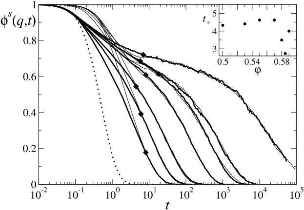
Figure 3: Simulation results for $\varphi=0.50$, $0.53$, $0.55$, $0.57$, $0.58$, $0.585$, $0.59$ (from left to right) at wave vector $qd=7.8$. Heavy solid lines are the results using Brownian dynamics, thin lines the results for Newtonian dynamics. For the latter curves, times $t$ have been multiplied by factors $t_{*}$ given in the inset. The dotted line is the BD result for $\varphi=0.01$, indicating the dilute limit of the correlation function. The solid diamonds indicate the points where Newtonian and Brownian dynamics results start to agree at a $2\%$ level.

In Fig. 3, results of the simulations are shown for different packing fractions $\varphi$. A wave vector $qd=7.8$ close to the first peak in the static structure factor has been chosen. Different values of $q$ show qualitatively similar scenarios. The thick solid lines in the figure are the simulation results for ‘Brownian’ dynamics simulations. Upon increasing $\varphi$, one observes the emergence of a two-step relaxation process at times long compared with typical liquid time scales. A typical relaxation curve for the dilute case, is exemplified by the dotted line in the figure, showing the BD simulation result for $\varphi=0.01$. From this, we read off a ‘microscopic’ relaxation time for the short-time relaxation of $t\approx 1$. The slow two-step relaxation pattern is usually referred to as structural relaxation and is a precursor of the approach to a glass transition at some $\varphi^{c}$. The scenario has been observed repeatedly in similar systems. In our simulations, we are able to follow the structural relaxation scenario for up to about five orders of increase in the relaxation time.

MCT predicts that the structural relaxation becomes, up to a common time scale $t_{0}$, independent on the type of microscopic motion that governs the relaxation at short times. To demonstrate that this is the case, Fig. 3 shows as thin lines the simulation results using Newtonian short-time dynamics. The data have been scaled in $t$ in order to match the BD data at corresponding packing fractions and at long times. Indeed, then the relaxation curves match within our error bars at times $t>10$, indicated by the diamond symbols in Fig. 3. Only at shorter times, the regime of non-structural relaxation can be identified by the different shapes of the BD and ND curves. According to MCT, the scale factor $t_{*}=t_{0}^{\text{BD}}/t_{0}^{\text{ND}}$ used to match the BD and ND data at long times should be a smooth function of $\varphi$, given by a constant in leading order close to $\varphi^{c}$. For our simulation results, the values are as shown in the inset of Fig. 3; they are compatible with a constant shift $t_{*}\approx 4.25$ within error bars. Only at $\varphi=0.58$ and $\varphi=0.585$ do we note a stronger deviation, the reason of which is unclear. The overall variance in $t_{*}(\varphi)$ is comparable to the one found in a similar study of a binary Lennard-Jones mixture Gleim et al. (1998).

We conclude that the time window $t>10$ deals with structural relaxation and thus comprises the regime where MCT predictions can be tested. At shorter times, deviations from those predictions must be expected. There are indications from theory Franosch et al. (1998); Fuchs and Th. Voigtmann (1999) and ND simulations Kob et al. (2002) that these deviations are larger in ND. We thus primarily discuss the BD data, which prove to be simpler to understand within an MCT description.

III.2 $\alpha$-process analysis

Figure 4: Comparison of the BD data for $\varphi=0.58$ (plus symbols) at wave vectors $qd=4.0$, $7.8$, $13.8$, and $19.8$ (from top to bottom). The long-time part of the data for $\varphi=0.55$ (I symbols), $0.57$ (crosses), $0.585$ (circles), and $0.59$ (star sybmols) is also shown, scaled in $t$ to match the long-time part of the $\varphi=0.58$ data. Solid lines are the MCT master curves for shifted $q_{\text{MCT}}$ (see text for details).

The second step of the two-step relaxation process, i.e. the decay of the correlators from their plateau value, is referred to as the $\alpha$ process. A prediction of MCT is that the shape of this $\alpha$ relaxation becomes independent on $\varphi$ in the limit $\varphi\to\varphi^{c}-0$. Thus, scaling the correlation functions for given $q$ and different $\varphi$ to agree at long times should collapse the data onto a master curve. Figure 4 demonstrates the validity of $\alpha$ scaling for the BD data at several wave vectors between $q=4.0$ and $19.8$. The scaling works as expected from the MCT discussion of the HSS Franosch et al. (1997) for $\varphi\leq 0.58$. The closer a state is to $\varphi^{c}$, the larger is the window where the correlator follows the $\alpha$-master function. The increase of the $\phi(q,t)$ above the master functions at shorter times is connected to the $\beta$ process, discussed below. For $\varphi=0.59$, $\alpha$ scaling breaks down at long times, $t\geq 500$. The reason for this is unclear, and cannot be understood within MCT. As observed by the orientational order parameter $Q_{6}$, the system did not show appreciable trends to crystallization in any of the analyzed simulation runs. Also for $\varphi=0.585$, some deviations from $\alpha$ scaling can be seen, particularly at $q=7.8$ and at around $t=1000$, which are not in agreement with the pre-asymptotic corrections to MCT $\alpha$ scaling. But in this case, the deviations are less pronounced than those at $\varphi=0.59$.

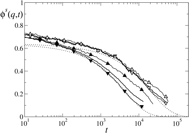
Figure 5: Demonstration of the variability between different simulation runs for the ND and BD simulations at $\varphi=0.59$. Data is shown for $qd=7.8$, with open (filled) symbols denoting BD (ND) results. Triangles indicate averages over a small subset of the data ($8$ out of $30$ sets for BD; $25$ out of $70$ for ND) only; inverted triangles are the averages over the remaining data sets. The solid lines without symbols are the total averages. Dotted lines indicate the time-scaled MCT $\alpha$-master functions.

The behavior of the long-time dynamics at these two densities, $\varphi=0.585$ and $0.59$ is not fully understood. We have tried to improve the statistical averaging by increasing the number of simulation runs. However, there appear to be two subsets among the runs: one where the $\alpha$-scaling violation is very pronounced, and one where the correlators instead follow the scaling behavior much closer. This happens in both the ND and the BD simulations, although the effect is more clearly seen in the ND case. Out of the $30$ data sets we have averaged in the BD case for $\varphi=0.59$, only $8$ show the scaling violation; in the ND case we have averaged over $70$ sets, with $25$ of them deviating from scaling. While Fig. 4 shows the data averaged over all simulation runs, Fig. 5 demonstrates the variation in $\alpha$-time scale between the two types of data sets, obtained by restricting the averaging to the number of data sets specified above. While we have no a priori justification to modify the averaging procedure in any way, it allows us to point out, that possibly some ‘rare’ events take place in the system at these high densities, which we cannot classify as crystallization events on the basis of $Q_{6}$, but which modify the dynamical long-time behavior in a distinct way. For the ND data, the $\alpha$-time scale varies by a factor of $2.5$ between the two cases. In the BD data, the effect is less pronounced, but still gives a factor of about $1.6$. As the dotted lines in Fig. 5 demonstrate, the majority of the data sets follows the predicted scaling rather closely, whereas a the remaining ones show significantly slower decay.

We have tried to analyze this finding further by looking at the distribution of squared displacements exhibited by all the particles, $P_{\text{MSD},t_{*}}(\delta r^{2})$, and its correlation with particle size. Here, $t_{*}$ is a fixed time, and the distribution is defined such that $\int P_{\text{MSD},t_{*}}(\delta r^{2})dr^{2}=\delta r^{2}(t_{*})$. We have fixed $t_{*}$ such that $\delta r^{2}(t_{*})=1.25d^{2}$. The distribution $P_{\text{MSD}}$ develops a non-Gaussian peak centered around its average value, whose width increases upon increasing the packing fraction. In some cases, we did observe a two-peaked distribution at $\varphi=0.59$, signifying that a certain amount of particles is displaced significantly less than average, i.e. that populations of ‘fast’ and ‘slow’ particles develop. This might be connected to the ‘rare events’ mentioned above, but we point out that this finding is unstable against improving the average over an increased number of simulation runs.

From the $\alpha$-scaling plot, Fig. 4, we infer the regime of $\alpha$-relaxation dynamics. Note that for $\varphi=0.58$, deviations from the $\alpha$-master curve due to $\beta$ relaxation are seen almost up to $t\approx 100$. Those will be analyzed later. Also shown in Fig. 4 are the MCT $\alpha$-master functions. If evaluated at the same $q$ as the simulation data, the description of the long-time dynamics is unsatisfactory, because the calculated stretching of the relaxation is too small. If we account for this error by shifting $q_{\text{MCT}}$ used in the calculations to higher values, we get good agreement, cf. the solid lines in Fig. 4. Note that the deviations from the $\alpha$-master curve set in at a time later than that where the ND and BD simulation results begin to overlap: e.g., the $q=7.8$ curve follows the $\alpha$-master curve only for times $t\gtrsim 100$, as can be inferred from Fig. 4. Still, the BD and ND curves for that state collapse within our error bars already for $t\gtrsim 20$, cf. Fig. 3. This underlines that the regime of structural relaxation identified in Fig. 3 is larger than that of the $\alpha$-decay regime observed in Fig. 4, i.e. that both simulation data sets show some extent of the MCT $\beta$-relaxation window.

The values of $q_{\text{MCT}}$ used in the fits of Fig. 4 are $q_{\text{MCT}}=5.0$ ($9.13$, $10.3$, $15.13$, $18.3$, $20.87$) for $q=4.0$ ($7.8$, $9.0$, $13.8$, $17.0$, $19.8$). These fit values are suggested by the analysis of the full curves pursued below, cf. Sec. IV. Comparing the fitted wave-vector values $q_{\text{MCT}}$ to those of the simulations, deviations in $q$ are in the range $10\%$ to $17\%$, except for $q=4.0$, where a $25\%$ deviation is needed to describe the $\alpha$-master function. The way we have adjusted $q_{\text{MCT}}$ ensures that the stretching of the correlators is described correctly. In contrast, a fit of the plateau values with the $\alpha$-master functions is difficult, since the latter are still not clearly visible in the simulation data even at $\varphi=0.59$. This will become more apparent in Sec. IV.

In all cases, the fitted wave-vector values are larger than the actual values, $q_{\text{MCT}}\geq q$. Since the $f^{s,c}(q)$ giving the plateau values decrease monotonically from unity at $q=0$ to zero at $q\to\infty$, this fit result is equivalent to stating that the MCT-calculated plateau values appear too high. Furthermore, the half-width of the $f^{s,c}(q)$ distribution is an estimate for the inverse localization length of a tagged particle. Hence the fit suggests that MCT underestimates the localization length of a tagged particle in the system slightly. There are two obvious reasons for such a mismatch in length scales: first, the softness of the particles in the simulation might, especially at high densities, give rise to some amount of particle overlap not possible in the HSS, rendering the effective localization of the particles slightly larger. According to Heyes Heyes (1997), the soft-sphere system used in our simulations can be well described within the hard-sphere limit and an effective hard-sphere diameter $d_{\text{eff}}=\int_{0}^{\infty}(1-\exp[-\beta V_{c}(r)])dr\approx d(1+\gamma_{e}/36)\approx 1.016$ (where $\gamma_{e}\approx 0.577$ is Euler’s constant), which differs from $d=1$ by less than $2\%$. But one has to keep in mind that the convergence of increasingly steep soft-sphere potentials towards the hard-sphere limit can be quite slow for the transport properties of the system Heyes and Powles (1998). Second, a difference in packing fractions between the simulation and the MCT calculation might become important in this respect. This arises, because within the PY approximation for the DCF, the MCT master curve is evaluated at the corresponding value for the critical packing fraction, $\varphi^{c}\approx 0.516<\varphi^{c}_{\text{sim}}$. As was pointed out in connection with Fig. 1, such a mismatch in $\varphi$ will affect the average particle distances, and thus an overall length scale. But since $\varphi^{c}_{\text{MCT}}<\varphi^{c}$ one would expect this to lead to an overestimation of the critical localization length, contrary to what we observe.

Figure 6: Example for Kohlrausch fits to the simulation data at $\varphi=0.58$ (symbols: Brownian dynamics, dots: Newtonian dynamics), $qd=4.0$, $7.8$, $9.0$, $13.8$, $17.0$, and $19.8$. The fit range was $t\geq 55$.

Traditionally, stretched-exponential (Kohlrausch) laws,

$$\phi^{s}(q,t)\approx A(q)\exp[-(t/\tau(q))^{\beta(q)}]\,,$$ (9)

are known to give a good empirical description of the $\alpha$ relaxation. Here, $A(q)$ is an amplitude factor, $\tau(q)$ the Kohlrausch time-scale of the $\alpha$ relaxation, and $\beta(q)<1$ is called the stretching exponent. These parameters in general depend on the observable under study, and in particular on the wave vector $q$. Fig. 6 demonstrates that the Kohlrausch laws can also be used to fit the $\alpha$-relaxation part of our simulation data. The figure shows as an example the state $\varphi=0.58$ for various wave vectors. One problem of the stretched-exponential analysis of the data is that the three parameters of the fit have a systematic dependence on the fit range. In particular, one has to restrict the fitting to such large $t$ that only $\alpha$ relaxation is fitted. For the fits shown, this range was chosen to be $t\geq 55$. The data deviate from the fitted Kohlrausch functions significantly only at shorter times; but there is a trend that these deviations set in just about the boundary of the fit range. This still holds if the fit is restricted to larger $t$ only, and judging from the fit quality for the remaining relaxation alone, one cannot determine the optimal choice of the fit range. It is thus particularly difficult to extract the regime of $\alpha$ relaxation from the Kohlrausch fits alone. On the other hand, from the MCT fits shown in Fig. 4 we expect corrections due to $\beta$ relaxation to set in at about $t\approx 100$. This in principle gives an indication of the maximum fit range to chose. Yet, Kohlrausch fits restricted to $t\geq 100$ did lead to an unsatisfactory scatter in the fit parameters $A(q)$ and $\beta(q)$. Thus an analysis of the $\alpha$ relaxation using Kohlrausch fits will erroneously include parts of the $\beta$ relaxation.

Figure 7: Critical nonergodicity parameter $f^{s,c}(q)$ calculated from MCT for the one-component hard-sphere system with PY approximation (solid line), and for a five-component polydisperse system (dashed line). Symbols are the amplitudes $A(q)$ from Kohlrausch fits to the data, where error bars estimate deviations depending on $\varphi$ and BD/ND. The dash-dotted line indicates $f^{s,c}(q)$, but transformed with the wave-number shift applied in the discussion of the dynamical data (see text for details).

This trend can be also identified comparing the obtained Kohlrausch amplitudes $A(q)$ with the plateau values $f^{s,c}(q)$. This comparison is shown in Fig. 7, where the MCT results for $f^{s,c}(q)$ are included. They have again been determined using the PY approximation to $S(q)$, but in agreement with Fig. 2, the values for $f^{s,c}(q)$ determined from MCT calculations based on the simulated $S(q)$ are indistinguishable from the ones shown on the scale of Fig. 7. For Kohlrausch fits to the $\alpha$-master function, and more generally to the $\alpha$-relaxation regime of the correlators only, $A(q)\leq f^{s,c}(q)$ should hold. Recalling the wave-number adjustment used in Fig. 4, we should even have $A(q)\leq f^{s,c}(q_{\text{MCT}}(q))$. This latter curve is included in Fig. 7 as the dash-dotted line, where the mapping $q\mapsto q_{\text{MCT}}$ was extended from the set of $q$ analyzed in this text to all $q$ via a quadratic interpolation. The relation $A(q)\leq f^{s,c}(q)$ is clearly violated for the fits here, especially at high $q$. It shows that the distinction between the $\alpha$ and $\beta$ regimes from the simulation data is difficult; increasingly so with increasing wave number.

It is reassuring that the Kohlrausch fits to BD and ND data yield values quite close to each other, apart from an overall shift in $\tau(q)$. This holds, as long as the fit ranges are chosen such as to fit approximately the same part of the relaxation. In Fig. 6, the ND curves have been added, again shifted by a scaling factor in $t$ given in the inset of Fig. 3. Note that, while in the ND curves one can identify a plateau from the data better than from the BD ones, still the KWW fits have a trend to give too high values of $A(q)$. Thus one has to be careful when extracting plateau values from the simulation data by such an analysis, even if the data seem to give a clear indication of the plateau.

Figure 8: Stretching exponents $\beta(q)$ from fits to the BD simulation data at $\varphi=0.58$ using Kohlrausch laws, Eq. (9). Error bars indicate deviations estimated from fits to ND data and to $\varphi=0.57$. The dashed horizontal line indicates the $b$ value calculated from MCT using the Percus-Yevick approximation for $S(q)$, $b\approx 0.583$, and the dash-dotted line is $b$ as determined from MCT with simulation-data input for $S(q)$, $b\approx 0.521$.

The stretching exponents $\beta(q)$ from the KWW fits are shown in Fig. 8. Again, we have included error bars indicating the deviations arising from fits to different $\varphi$ or to ND as opposed to BD simulation data. $\beta(q)$ increases with decreasing $q$, and this increase is compatible with $\beta(q)\to 1$ for $q\to 0$, as expected from theory Fuchs et al. (1992). According to MCT, $\beta(q)$ should approach the von Schweidler exponent $b$ as $q\to\infty$ Fuchs (1994). The value of $b$ is calculated from the MCT exponent parameter $\lambda$, and for the HSS using the PY-DCF is $b\approx 0.583$, shown as a dashed line in Fig. 8. We observe that the fitted $\beta(q)$ fall below this value for large $q$, even if the fits are less reliable there, due to the low amplitudes $A(q)$ at high $q$. To estimate the error of the theory prediction for $b$, we have also calculated this exponent from MCT using the simulated data as input for $S(q)$. According to the values of $\lambda$ reported in connection with Fig. 2, we get $b\approx 0.56\pm 0.04$. The lower bound for $b$ thus obtained is indicated in Fig. 8 as the dash-dotted line. Taking into account this uncertainty, the behavior of the fitted $\beta(q)$ agrees well with what is expected from theory. In the further discussion, we will fix $\lambda$ to its value derived from the PY approximation, $\lambda=0.735$. Since the shape of the correlation functions in the $\beta$ regime is in the asymptotic limit fixed by $\lambda$, some deviations in the fits described below are to be expected in this time window.

III.3 Analysis of $\alpha$-relaxation times

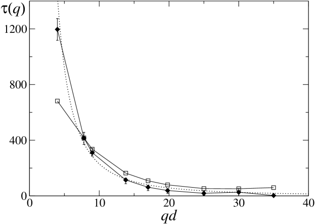
Figure 9: $\tau(q)$ from Kohlrausch fits, Eq. (9), to the BD data at $\varphi=0.58$ (diamonds) and at $\varphi=0.59$ (squares; scaled by a factor of $0.021$). Error bars estimate the uncertainty from the fits, see text for details. The dotted line shows a $1/q^{2}$ law.

The $q$-dependence of the $\alpha$-relaxation times at fixed $\varphi$ can best be analyzed from the $\tau(q)$ extracted from Kohlrausch fits. In Fig. 9, we report values for $\tau(q)$ for such fits to the BD data at $\varphi=0.58$ as the diamond symbols. If one instead fits the ND data, or data at $\varphi=0.585$ or $0.57$, the $q$-dependence is the same up to a prefactor and up to small deviations. These deviations are indicated by the size of the error bars in Fig. 9. The data closely follow a $1/q^{2}$ dependence for small $q$, indicated by the dotted line. This is in agreement with earlier MCT predictions for the hard-sphere system Fuchs et al. (1992). For $q\to\infty$, one expects from MCT $\tau(q)\sim q^{-1/b}$. But since $b$ is close to $1/2$, we cannot distinguish this behavior reliably from a $1/q^{2}$ law due to the noise of the data at large $q$.

Fits to the BD data at $\varphi=0.59$ reveal significant deviations from the behavior at $\varphi\leq 0.585$ at small $q$. This can be deduced from the square symbols in Fig. 9. They have been scaled by a constant factor in order to match the value obtained from the $\varphi=0.58$ fit at $q=7.8$, since there the MCT analysis works best, as will be shown below. At smaller $q$, the increase of $\tau(q)$ with decreasing $q$ is suppressed for the $\varphi=0.59$ data in comparison to the variation in $\tau(q)$ observed for smaller $\varphi$.

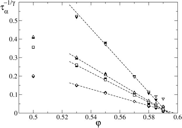
Figure 10: Plots of $\tau_{\alpha}^{-1/\gamma}$ for wave vectors $qd=4.0$ (diamonds), $7.8$ (squares), $9.0$ (up triangles), and $13.8$ (down triangles); using $\gamma=2.46$. (a) Results for the simulation data using Brownian dynamics (open symbols) and Newtonian dynamics (filled symbols). The values of $\tau$ for the latter have been multiplied by $4.5$ for this plot. Dashed lines are linear fits to the Brownian dynamics data in the range $0.54\leq\varphi\leq 0.58$.

For a discussion of the density dependence of the $\alpha$-relaxation time, the $\tau(q)$ from the stretched-exponential fits are less reliable, since the Kohlrausch fits suffer from larger uncertainties at lower $\varphi$, where the $\alpha$- and $\beta$-regimes are even less well separated. But we can operationally define a time scale $\tau_{\alpha}$ for the decay of the correlation functions as the point where the correlators have decayed to $10\%$ of their initial value, $\phi^{s}(q,\tau_{\alpha})=0.1$. For small enough $q$ where $f^{s,c}(q)$ is still much larger than $0.1$, $\tau_{\alpha}$ is a useful measure for the $\alpha$-process time scale. In the asymptotic regime, where $\alpha$ scaling holds, it follows the $\alpha$-scaling time defined within MCT up to a constant. Thus MCT predicts a power-law divergence of $\tau_{\alpha}$ close to $\varphi^{c}$ of the form $|\varphi-\varphi^{c}|^{-\gamma}$ for not too large $q$, $q\leq 15$, say. To test this prediction, we plot in Fig. 10 the quantity $\tau_{\alpha}^{-1/\gamma}$, which should yield a straight line crossing zero at $\varphi^{c}$. Since the region of validity of this asymptotic result is not known a priori, a determination of the correct value of the exponent $\gamma$ on the basis of such rectification plot suffers from large errors. Therefore, let us fix $\gamma\approx 2.46$, the value calculated by MCT using the PY approximation. Due to the uncertainty in determining $\lambda$ mentioned above, slightly different values of $\gamma$ cannot be ruled out. One gets $\gamma\approx 2.66$ as an upper bound when using the upper bound for $\lambda$ given above for the MCT result based on the simulated $S(q)$. This value of $\gamma$ is also quite close to what one gets Fuchs et al. (1992) using the Verlet-Weis-corrected PY structure factor Verlet and Weis (1972). Figure 10 shows rectification plots for both Brownian and Newtonian dynamics simulation data for $4.0\leq q\leq 13.8$. For the latter, the values of $\tau_{\alpha}$ have been multiplied by $4.5$, consistent with the shift in the overall time scale, cf. inset of Fig. 3. Fits to straight lines give $\varphi^{c}$ values that are consistent with each other for $q\geq 7.8$ and both microscopic dynamics, if one restricts the fit range to high enough $\varphi$ and omits the highest densities, where alpha scaling breaks down, $0.54<\varphi<0.58$ in our case. From this, one gets $\varphi^{c}\approx 0.594\pm 0.001$. The data for $q=4.0$ give a somewhat higher value, $\varphi^{c}\approx 0.598\pm 0.001$, again the same for Newtonian and Brownian dynamics. This difference is outside the error bars of the analysis and thus not in accord with MCT. Since the discrepancy is the same for both types of short-time dynamics, we conclude that indeed the structural relaxation deviates from the MCT prediction systematically at small $q$.

The range of distances $\varepsilon$ to the critical point, in which we can fit the time scales consistently with a power law, is roughly $|\varphi-\varphi^{c}|/\varphi^{c}\leq 0.07$. This agrees with what is expected from a discussion of the asymptotic MCT results for the hard-sphere system Franosch et al. (1997): For the time-scales extracted from the numerical MCT results, we have to restrict the linear fit to $\varphi_{\text{MCT}}\geq 0.48$, where the critical point is $\varphi^{c}_{\text{MCT}}\approx 0.516$. Below $\varphi_{\text{MCT}}=0.48$, one finds deviations from the straight lines in the rectification plot; typically the results fall below the asymptotic straight line in such a plot. If one tries to fit a larger range in $\varphi_{\text{MCT}}$, the thus estimated $\varphi^{c}$ will be higher than the correct one. For example, we get $\varphi^{c}\approx 0.519\pm 0.0015$ when fitting in the range $\varphi_{\text{MCT}}\geq 0.4$. It is reassuring that the deviations from the linear behavior seen in Fig. 10 for the simulation results occur in the same direction as found for the MCT results.

At large $q$ and at the highest packing fractions studied, the $\tau_{\alpha}$ from the simulations are systematically smaller than what is expected from the power-law extrapolation. This suggests that the local relaxation dynamics of the system very close to the transition would be faster than expected within the theory. However, the full theory analysis presented below suggests the opposite, indicating that at these high $q$, the operational definition of $\tau_{\alpha}$ we have chosen for simplicity no longer works.

III.4 $\beta$-process analysis

We now test some of the predictions MCT makes for the $\beta$-relaxation regime, where the correlators remain close to their plateau values. The time window where the asymptotic solution holds, extends in $t$ upon control parameters approaching the transition point, i.e. $\varphi\to\varphi^{c}$. The leading deviation from the plateau value is of order $\sqrt{|\sigma|}$, where $\sigma$ is called the distance parameter, and

$$\sigma =C\cdot\varepsilon\,, \varepsilon =(\varphi-\varphi^{c})/\varphi^{c}\,,$$ (10)

in leading order is the linearized distance in control-parameter space. The leading-order asymptotic result is called factorization theorem, and it can be written for the tagged-particle correlator as

$$\phi^{s}(q,t)=f^{s,c}(q)+h^{s}(q)G(t)\,.$$ (11)

Here, $G(t)$ is a universal function depending only on the parameters $\lambda$, $\sigma$, and a fixed ‘microscopic’ time scale $t_{0}$. The expansion is valid on a time scale $t_{\sigma}=t_{0}|\sigma|^{-1/(2a)}$ that diverges upon approaching the transition point. On this time scale, all wave-vector dependence is factorized off from the time dependence, and contained in the critical amplitudes $h^{s}(q)$ and the plateau values $f^{s,c}(q)$. All parameters can be calculated within MCT, but as we have seen above, extracting them from the simulation data is not straightforward. Kob et al. Gleim and Kob (2000) have introduced a test of the factorization property that can be performed without fitting any of the $q$-dependent quantities to the data: they considered

$$X(q,t)=\frac{\phi^{s}(q,t)-\phi^{s}(q,t^{\prime})}{\phi^{s}(q,t^{\prime})-\phi^{s}(q,t^{\prime\prime})}\,.$$ (12)

If fixed times $t^{\prime}$ and $t^{\prime\prime}$ are chosen inside the $\beta$ regime, the factorization theorem gives $X(q,t)\equiv X(t)=x_{1}G(t)-x_{2}$ for $t$ inside the $\beta$ regime, with constants $x_{1}$ and $x_{2}$ not depending on $q$. Therefore, if the factorization theorem holds, plotting $X(q,t)$ for various $q$ collapses the curves in the $\beta$ window, without the need for fitting wave-vector dependent amplitudes and plateau values.

Figure 11: (a) $\beta$ analysis of the BD simulation data at $\varphi=0.58$: the curves marked by symbols show $X(q,t)=(\phi^{s}(q,t)-\phi^{s}(q,t^{\prime}))/(\phi^{s}(q,t^{\prime})-\phi^{s}(q,t^{\prime\prime}))$ with $t^{\prime}=8.234$, $t^{\prime\prime}=20.8075$. Wave vectors are $qd=4.0$ (diamonds), $qd=7.8$ (squares), $qd=9.0$ (up triangles), $qd=13.8$ (down triangles), and $qd=17.0$ (circles). The dashed line is the equivalent of the MCT $\beta$ correlator, see text for details. The dash-dotted line indicates the plateau value estimated from the root of the $\beta$ correlator. (b) Same for the ND simulation data, $t^{\prime}=2.31$ and $t^{\prime\prime}=5.845$.

We have performed this test for our simulation data for both BD and ND. Figure 11a shows the results for the BD simulation at $\varphi=0.58$, with $t^{\prime}=8.234$ and $t^{\prime\prime}=20.8075$. One observes that the data nicely collapse for $5\leq t\leq 40$. Additionally, the figure shows the $X(t)$ constructed from the MCT $\beta$ correlator as a dashed line. Here, two constants $x_{1}$ and $x_{2}$, and the time scale $t_{\sigma}$ have been fitted. The value of $\lambda$ has been taken from the theory as explained above, $\lambda=0.735$. The same analysis is carried out for the ND data in Fig. 11b. Here, we have fixed $t^{\prime}_{\text{ND}}=2.31\approx t^{\prime}/3.5$ and $t^{\prime\prime}_{\text{ND}}=5.845\approx t^{\prime\prime}/3.5$, since at $\varphi=0.58$ the shift in time scales between BD and ND is a factor of about $3.5$, cf. inset of Fig. 3. Again the data collapse in an intermediate window $2\leq t\leq 15$. The upper end of this window is consistent with the one found for the BD analysis, i.e. $15\approx 40/3.5$. The lower end of the window where $\beta$ scaling holds for the ND data is higher than what would correspond to the BD $\beta$ window. Thus preasymptotic corrections are stronger in the ND case. The fit using the MCT $\beta$ correlator is not as good as it is for the BD case. Since the distance to the critical point does not change between BD and ND, we have used the $t_{\sigma}$ determined from the above fit to the BD data also here. Furthermore, since we have chosen $t^{\prime}_{\text{ND}}$ and $t^{\prime\prime}_{\text{ND}}$ in accordance with the values of $t^{\prime}$ and $t^{\prime\prime}$ for the BD analysis, the constants $x_{1}$ and $x_{2}$ should be the same; this is roughly fulfilled by our fit.

The fits to both data sets have been performed such as to obey the ‘ordering rule’ for the corrections to $\beta$ scaling Franosch et al. (1997): a curve that falls below another one for times smaller than the $\beta$ window, will also do so for time larger than the $\beta$ regime, since the corrections both at small and at large times are determined by the same $q$-dependent correction amplitudes. Thus the ordering of wave vectors on both sides of the scaling regime is preserved. This prediction of MCT is fulfilled by the BD simulation data, as can be seen in Fig. 11a. For the ND data, we cannot fulfill this ordering at both short and long times with reasonable fit parameters. At shorter times, one finds that e.g. the $q=7.8$ and $q=9.0$ curves rise above the $\beta$-correlator curve, in violation of the ordering rule. We thus conclude that at this point, microscopic deviations set in for the ND simulations that are stronger than the ones in the BD data. The point $q_{0}$ where the corrections to $\beta$ scaling change sign can be inferred from Fig. 11 to be $q_{0}\approx 9/d$. It is independent on the type of short-time dynamics, in excellent agreement with the predicted universality of structural relaxation, and in particular the correction-to-scaling amplitudes. The numerical value of $q_{0}$ also agrees well with that found in an analysis of the MCT results for the tagged-particle correlator in a hard-sphere system Fuchs et al. (1998), where the change occurs at $q_{0,{\text{MCT}}}\approx 9.3/d$.

The $\beta$ correlator for short times approaches the critical power law, $G(t)\sim t^{-a}$. Comparing this asymptote with the fitted $\beta$ correlator in Fig. 11, one finds that the $t^{-a}$ law already deviates from the $\beta$ correlator at $t\approx 1$ for the BD data, and at $t\approx 0.3$ for the ND data. Thus the critical decay cannot be identified from the simulation data. This is typical for most experimental data Götze (1999). One thus has to be careful when extracting the exponent $a$ from an analysis of the $\beta$ relaxation.

Let us from now on restrict the discussion to the BD data set. For the ND data, deviations from the MCT predictions occur in the early part of the $\beta$ regime, and thus the theory can explain a larger part of the BD curves than it can do for the ND ones. For the analysis of the long-time universality of the dynamics outlined above, we conclude that these deviations are not a feature of the glassy dynamics. It is known that MCT treats the short-time dynamics insufficiently Kob et al. (2002), and that Brownian dynamics typically stays closer to the MCT scenario for a larger time window than the corresponding Newtonian dynamics Franosch et al. (1998); Fuchs and Th. Voigtmann (1999).

IV Full MCT Analysis

Figure 12: MCT (solid lines) and simulation results (symbols) for $\phi^{s}(q,t)$. For the simulation data, packing fractions are $\varphi=0.50$, $0.53$, $0.55$, $0.57$, $0.58$, $0.585$, and $0.59$ (from left to right), and $qd=7.8$. For the MCT results, packing fractions have been adjusted to $\varphi_{\text{MCT}}=0.445$, $0.47$, $0.484$, $0.499$, $0.505$, $0.508$, and $0.5135$, and the wave number has been adjusted to $q_{\text{MCT}}d=9.13$; see text for details.

Figure 13: MCT and simulation data for $\phi^{s}(q,t)$ with symbols and packing fractions as in Fig. 12, but for $qd=9.0$, adjusted in the MCT calculations to $q_{\text{MCT}}d=10.3$.

Figure 14: MCT and simulation data for $\phi^{s}(q,t)$ with symbols and packing fractions as in Fig. 12, but for $qd=13.8$ ($q_{\text{MCT}}d=15.1$).

Figure 15: MCT and simulation data for $\phi^{s}(q,t)$ with symbols and packing fractions as in Fig. 12, but for $qd=17.0$ ($q_{\text{MCT}}d=18.3$).

We now turn to a full data analysis, i.e. a comparison of the complete simulation data with the solutions of the full MCT equations for a hard-sphere system.

In the MCT picture, the glassy dynamics of the hard-sphere system is mainly driven by density fluctuations over the length scale of the mean nearest-neighbour distance, i.e. with wave numbers close to that of the first sharp diffraction peak in $S(q)$. We therefore begin the analysis by focusing on the data for $q=7.8$. The results of our full-MCT fits to the BD simulation data are shown in Fig. 12. To achieve this and the following fits, we have adjusted $\varphi_{\text{MCT}}$ for each curve and allowed the wave number $q_{\text{MCT}}$ to vary slightly with respect to the correct value $q$. No other parameters have been adjusted. As noted above, the $q$-shift to some extent accounts for a mismatch in length scales between the simulation and the theory predictions. The adjustment of $\varphi_{\text{MCT}}$ on the other hand accounts for the known error in $\varphi^{c}$. We will discuss the relation of the fitted $\varphi_{\text{MCT}}$ to the correct packing fraction $\varphi$ below.

The fit shown in Fig. 12 demonstrates that the theory can, with these modifications allowed, account for the dynamics of the hard-sphere system in a time window of over four decades on a $10\%$ error level. Only at larger times, $t\approx 10^{4}$ in our units, i.e. at the highest packing fraction studied, systematic deviations are observed. The simulation for this packing fraction shows slower dynamics than expected from the theory. Also the shape of the final decay is different, as noted above in connection with $\alpha$ scaling. On the short-time side, the MCT description works down to a time $t\approx 1$. At shorter times, it is still almost quantitative, but one observes a different curve shape. The simulation data appears more strongly damped than the MCT curves. This is to be expected, since neglecting the regular part of the memory kernel in Eq. (3b) will lead to such deviations at short times. We could have accounted for this partly by choosing a higher value of $\nu$ in Eq. (3b), but we have not done so since we are not concerned with the short-time dynamics in this work.

Once the fit for $q=7.8$ was completed to fix the empirical relation $\varphi_{\text{MCT}}(\varphi)$, we have analyzed data for other wave numbers up to $q=30$, hereby fixing the relation $q_{\text{MCT}}(q)$. Typical results for $q\leq 17$ are exhibited in Figs. 13 to 15. Note that the only parameter that was adjusted for these fits is the wave number, $q_{\text{MCT}}$. This way, Figs. 13 to 15 demonstrate how MCT is able to reproduce the wave-vector dependent changes in the structural-relaxation window. At even higher $q$, it becomes too difficult to judge the fit quality, since the $f(q)$ are close to zero there. Connected with this is the growing influence of the microscopic regime, $t\leq 1$, on the main part of the decay of the correlators with increasing $q$. For $q=17$ and the highest packing fractions, already about $60\%$ of the decay of $\phi^{s}(q,t)$ from unity to zero are made up of such microscopic dynamics. Consequently, the errors made in its description are to be seen more explicitly in Fig. 15 than in Fig. 12.

Apart from this, also the fits at $q>7.8$ using the full-MCT results are quite satisfactory in the time window $1\leq t\leq 10^{4}$, save the highest simulated density, for which errors are largest and extend down to $t\approx 10$ for $q=13.8$ and $17$, cf. Figs. 14 and 15. One notices a trend that the $\alpha$-relaxation dynamics becomes slower in the simulation data than expected from the MCT fits, i.e. the local dynamics is slower than one estimates in the theory. The finding can probably not fully be attributed to the incorrect structure-factor input used, since a recent study of binary hard-sphere mixtures reported a similar discrepancy for the $q$-dependence of the $\alpha$-relaxation times even when basing MCT on the ‘correct’ simulated $S(q)$ as input Foffi et al. (2004). The same trend is also apparent in the full-MCT analysis of a binary Lennard-Jones mixture Kob et al. (2002).

Figure 16: Plot of $\varphi_{\text{MCT}}$ vs. $\varphi$ for the fits shown in Figs. 12–15, 17 and 18 (diamonds). The dashed line is a linear fit, $\varphi_{\text{MCT}}\approx 0.81\varphi+0.037$. The circles are for the independent fit of the MSD, Fig. 19. The dotted horizontal line indicates the calculated critical point, $\varphi^{c}\approx 0.516$.

Having established the overall quality of the MCT description for the structural dynamics on length scales smaller and comparable to the typical particle-particle distance, let us now investigate the adjustment in $\varphi_{\text{MCT}}$ needed to achieve this level of agreement. A plot of $\varphi_{\text{MCT}}$ vs. $\varphi$ is shown in Fig. 16 (diamond symbols). The figure reveals that the relation is close to linear, and thus the nontrivial variation of the relaxation curves close to the singularity $\varphi^{c}$ has not been put in ‘by hand’ through the fitting parameter $\varphi_{\text{MCT}}$. We can estimate the correct value of the glass-transition packing fraction by a linear fit to the $\varphi_{\text{MCT}}$-versus-$\varphi$ curve. Using the calculated value $\varphi^{c}_{\text{MCT}}\approx 0.516$, we get $\varphi^{c}\approx 0.594$. This value is nicely consistent with the one obtained from the $\alpha$-scale analysis of the data, cf. Fig. 10, and also from an earlier analysis of the simulations Puertas et al. (2002). Note that it differs from the result obtained from MCT based on the simulated $S(q)$, $\varphi^{c}\approx 0.585$ by less than $2\%$. The slope of the linear fit in Fig. 16 is not equal to unity, and its zero is shifted. If one considers the connection of the distance parameter $\sigma$ of MCT to the control-parameter distance $\varepsilon$, this translates into an error of the leading-order constant of proportionality $C$ in Eq. (10). From Fig. 16 we conclude that the value calculated from MCT, $C_{\text{MCT}}\approx 1.54$ Franosch et al. (1997), is in error by about $20\%$, $C\approx 1.2$.

Figure 17: MCT and simulation data for $\phi^{s}(q,t)$ with symbols and packing fractions as in Fig. 12, but for $qd=4.0$ ($q_{\text{MCT}}d=5.0$).

For small $q$, the MCT description of the data shows larger quantitative errors, while it remains qualitatively correct. This is exhibited by the fits done for $q=4.0$, Fig. 17. Again, only $q_{\text{MCT}}$ was allowed to vary, while the $\varphi_{\text{MCT}}$ have been determined from the $q=7.8$ fit shown in Fig. 12. While for this latter fit, the MCT fits reproduce the $\alpha$-relaxation times rather well, this is not the case for the $q=4.0$ fit at $\varphi\geq 0.57$. Instead, one observes a systematic trend for the simulation data to decay increasingly faster than the MCT curves with increasing $\varphi$. In addition, the deviations observed in the $\beta$-relaxation window, while still within a $10\%$ level, are larger for $q=4.0$ than they are for $q\geq 7.8$. Even more, it was necessary to allow for a $25\%$ deviations between $q_{\text{MCT}}$ and $q$, whereas this deviation was less than $17\%$ for all other fits. This last finding suggests that the $f^{s,c}(q)$-versus-$q$ curve calculated within MCT is too broad. It is common to express deviations of the $\phi^{s,c}(q,t)$-versus-$q$ curve at fixed $t$ from a Gaussian at small $q$ in terms of the non-Gaussian parameter, $\alpha_{2}(t)$. These non-Gaussian corrections are reproduced qualitatively correct by MCT, but with an error in magnitude. One finds $\alpha_{2}(t)\leq 0.3$ in the theory Fuchs et al. (1998), while for our simulation, $\alpha_{2}(t)$ reaches values up to $2.5$ in both BD and ND, which is in agreement with similar simulation results for other systems Kob and Andersen (1995). But note that for times where $\phi^{s}(q,t)$ is close to its plateau value $f^{s,c}(q)$, both the MCT and the simulation value of $\alpha_{2}(t)$ are positive. Thus the underestimation of $\alpha_{2}$ in the theory would let the $f^{s,c}(q)$-versus-$q$ curve appear too narrow, opposite to what is observed from our fits. We thus conclude that non-Gaussian corrections as expressed through $\alpha_{2}(t)$ and the quantitative error MCT makes in expressing them cannot be alluded to to explain the deviations observed at $q=4.0$. Let us point out that the deviations discussed above do not depend significantly on the fact that we have based the MCT calculation on the PY-DCF. Using the simulated structure factor with MCT gives correlation functions $\phi^{s}(q,t)$ that behave qualitatively as the ones shown here.

Figure 18: Comparison of the mean-squared displacements $\delta r^{2}(t)$ from simulation and MCT calculations; all fit parameters have been taken from Fig. 12. In addition, the MCT curves have been multiplied by $1.1$ to account for an error in localization length; see text for details.

It is instructive to extend this analysis towards the mean-squared displacement data. Since the MSD is given through a memory kernel that basically is a $q\to 0$ limit of the tagged-particle-correlator memory kernel, Eq. (7), its analysis can be viewed as the $q\to 0$ extension of the above fitting procedure.

We report the BD simulation data for the MSD, together with the MCT curves according to the correlation functions shown above, in Fig. 18. For the MSD, no wave number is to be adjusted, and in this sense, the MCT results of Fig. 18 are not fitting results, but rather consequences of the analysis done for $q=7.8$, shown in Fig. 12. We have, however, adjusted a global length scale in this plot, in order to better fit the localization plateau visible in the data. The MCT curves have been scaled up by a factor of $1.1$, which accounts for a $5\%$ underestimation of the localization length by the theory. Note that at short times, $t<1$, the description of the data using MCT is of similar quality as discussed above. In particular, the MSD plot reveals that the BD simulation still resembles a Newtonian short-time dynamics, though strongly damped: the MSD roughly follows a $\delta r^{2}\sim t^{2}$ law for $10^{-2}<t<10^{-1}$, and not a $\delta r^{2}\sim t$ law as would be expected for short-time diffusion in a strictly Brownian system. Theory and simulation do not match at short times because of the scale factor applied. For long times, a qualitatively similar picture emerges as for $q=4.0$, regarding the variation of the $\alpha$-relaxation times with $\varphi$, now showing through a displacement of the long-time diffusive straight lines in the $\delta r^{2}(t)$ plot. As for $q=4.0$, the quality of the MCT description of the $\beta$-relaxation regime similarly is worse than for $q\geq 7.8$. But for the MSD, all deviations are larger than for $q=4.0$, especially in the $\alpha$-relaxation regime.

Figure 19: Comparison of the mean-squared displacements $\delta r^{2}(t)$ from simulation and MCT calculations. In this plot, values $\varphi_{\text{MCT}}$ used for the MCT calculations have been adjusted to fit the long-time diffusion regime of the simulated $\delta r^{2}(t)$; the values are $\varphi_{\text{MCT}}=0.438$, $0.46$, $0.478$, $0.494$, $0.502$, $0.503$, and $0.511$ for $\varphi=0.50$, $0.53$, $0.55$, $0.57,$ $0.58$, $0.585$, and $0.59$, respectively.

Before investigating the $\alpha$-relaxation regime in more detail, let us note that, all deviations taken aside, the shapes of the MSD curves as predicted by MCT are qualitatively correct. To substantiate this statement, Fig. 19 shows an independent fit of the MSD using MCT. Instead of fixing the $\varphi_{\text{MCT}}$-versus-$\varphi$ relation from the data at $q=7.8$, as was done above, in this case this relation was determined from the MSD alone. It is noteworthy that by correcting the error in the $\alpha$-relaxation time scale observed before, also the description of the $\beta$-relaxation window improves. In particular, we did not scale the MCT results as we have done in Fig. 18. The values $\varphi_{\text{MCT}}(\varphi)$ used in Fig. 19 are reported in Fig. 16 as the circle symbols. They also lie on a straight line, which is shifted downward somewhat with respect to the original relation deduced from the above fits. In turn, an estimation of $\varphi^{c}$ from the mean-squared displacement, i.e. from the diffusivities, yields a value that is too high, viz.: $\varphi^{c}\approx 0.598\pm 0.003$. This is a typical result also found in other simulations Foffi et al. (2004), but not in accord with MCT. But note that the estimations for $\varphi^{c}$ are quite close to each other, so the deviations can be regarded as indications of error margins. As a side remark, let us note that the parameters from the independent fit to the MSD presented in Fig. 19 could be used to improve the description of the $q=4.0$ case somewhat, but not completely. One concludes that the MCT description of the single-particle structural relaxation smoothly deteriorates for decreasing $q$.

Figure 20: Self-diffusion coefficients $D$ as a function of the packing fraction $\varphi$, as obtained from the Brownian dynamics simulation (diamonds, with connecting lines to guide the eye) and from MCT calculations (solid line). The dashed line indicates the MCT asymptote, $D\propto(\varphi^{c}-\varphi)^{\gamma}$.

The deviations in the $\alpha$-relaxation regime, i.e. the long-time diffusive regime, that arise for the MSD can be analyzed more clearly by looking at the long-time self-diffusion coefficient $D(\varphi)$ itself. Here, $D$ has been determined from the simulations by the Einstein relation, $\delta r^{2}\sim 6Dt$ for large $t$, at times $t$ where $\delta r^{2}$ is of the order of $10$ squared particle radii. The results for the BD simulations are shown in Fig. 20 as the diamond symbols. In contrast, the MCT calculation, plotted in the figure as a solid line, shifted according to the relation $\varphi_{\text{MCT}}(\varphi)$ used in the above discussion, systematically falls below these values. The relative error in $D$ is less than $20\%$ up to $\varphi\approx 0.55$, increases to $80\%$ at $\varphi=0.58$, and reaches a factor of $4$ at $\varphi=0.59$. The two curves could be matched within the error bars by further shifting the MCT results along the $\varphi$ axis by less than $1\%$, which is basically what has been done in Fig. 19. But let us stress that there is no theoretical justification for doing so.

MCT predicts a power-law asymptote for $D$ with the same exponent $\gamma$ that applies for the divergence of the $\alpha$-relaxation times, $D\propto|\sigma|^{\gamma}$. This asymptote is included in Fig. 20 for the MCT results as a dashed line. It is also possible to fit the simulation data with such a power-law. We have restricted these fits to $\varphi\geq 0.55$ and have omitted the value at $\varphi=0.585$. If we fix the exponent to the theoretical value, $\gamma\approx 2.46$, we get reasonable agreement with a fitted $\varphi^{c}\approx 0.599$, in agreement with the above observation. If we, on the other hand, also determine $\gamma$ from the fit to $D(\varphi)$, the result is $\varphi^{c}\approx 0.597$ with $\gamma\approx 2.24$. It is a typical observation from simulation and experiment is that an independent determination of $\gamma$ from the diffusion coefficient yields a different value than that obtained from the analysis of the density correlators Kob and Andersen (1994). From the comparison of the MCT results with the asymptotic prediction in Fig. 20, it is, however, clear that the asymptotic law only holds for $D<10^{-3}$, i.e. for $\varphi\geq 0.58$ for our simulations. Thus a large part of the fitted simulation data is outside the asymptotic regime for this power law, and the fit yields an effective exponent rather than the true $\gamma$.

Figure 21: Product $D\cdot\tau(q)$ at wave vector $qd=7.8$ for the BD simulation (crosses, connected by lines to guide the eye), and for the MCT curves (solid line). The latter curve has been transformed along the horizontal axis according to Fig. 16. The inset shows a magnification of the MCT result versus $\varphi_{\text{MCT}}$.

The above results indicate that with $\varphi$ increasing close to $\varphi^{c}$, a decoupling of the diffusion time scale, as seen from the mean-squared displacement, from the density-fluctuation-relaxation time scale, as seen in the density correlation functions, sets in. This can be illustrated without referring to any fits by plotting the product $D\tau(q)$ of the diffusion coefficient $D$ and the $\alpha$-relaxation time scale Kob (2003). For the latter, let us choose the value obtained for $q=7.8$, as a typical representative of the local-order length scale. Figure 21 shows as symbols the results from the BD simulation. One notices an increase in $D\tau$ by a factor of $2$ to $3$ within the density range covered by the simulations. We have also checked that this holds similarly for $q=4.0$ and $q=9.0$. The corresponding MCT result is shown as the solid line in Fig. 21, which is magnified in the inset of the figure. Here, the product $D\tau$ also increases with increasing $\varphi$ close to $\varphi^{c}$, but only on the order of $10\%$. One thus concludes that there is a rather large quantitative error in this quantity, although not necessarily a qualitative one. MCT predicts that $D\tau$ approaches a finite value as $\varphi\to\varphi^{c}$. As to whether $D\tau$ diverges or stays finite at $\varphi^{c}$ in the simulation, our data remain inconclusive. Note that the values for the highest two packing fractions simulated are relatively uncertain, as the scatter in $D\tau$ indicates.

V Polydispersity Effects

Up to now, we have neglected the fact that the simulated system is not strictly a single-component system. Instead, some size polydispersity was needed in order to avoid crystallization. In this section, we give a brief account of how much we expect this small polydispersity to affect the results discussed above.

Figure 22: Averaged static structure factor $S(q)$ for a monodisperse system (dashed lines) and the polydisperse system studied in this work (solid lines) at the same state point. The main figure shows the simulation results at $\varphi=0.54$. The inset shows the Percus-Yevick $S(q)$ at the respective MCT-critical packing fractions $\varphi_{\text{MCT}}^{c}$, for both the monodisperse (dashed) and a five-component system (solid lines).

We first examine the influence of polydispersity on the equilibrium fluid structure. To this end, we have simulated a monodisperse system of the same soft spheres as used in the polydisperse simulations. We found such simulations possible for packing fractions up to $\varphi\approx 0.54$, above which crystallization as monitored by $Q_{6}$ sets in rather quickly. The static structure factor $S(q)$ at this state point is compared to the one from the polydisperse system at the same density in Fig. 22. As expected, the polydisperse system exhibits less pronounced ordering, visible in reduced oscillation amplitudes in $S(q)$. The effect is well explained by the PY approximation, as the inset of Fig. 22 demonstrates. There, the (total-density) structure factor for the one-component hard-sphere system is compared with that obtained from the five-component mixture introducted in Sec. II.2. One might expect the visible differences in the monodisperse and the polydisperse $S(q)$, however small, to affect the MCT results for $\varphi^{c}$. This would be true if both systems were treated as one-component systems. But it is not necessarily true for a full calculation of multi-component MCT, using the full matrix of partial structure factors instead of only the averaged $S(q)$, as we will discuss now.

Let us compare the results obtained for $f^{s,c}(q)$ for the one-component system with those of the five-component system mentioned above. This comparison is included in Fig. 7, where the dashed line shows the averaged $f^{s,c}_{\text{pd}}(q)$ according to Eq. (8). The thus obtained curve is slightly narrower than the solid curve, representing the result of the one-component calculation. Accordingly, the average localization length increases slightly, by about $4\%$. From the above discussion we conclude that this is a change in the right direction, but not enough to account for the wave-number shift we had to apply to describe the density correlation functions with the one-component system. Comparing with the Kohlrausch amplitudes $A(q)$ also shown in Fig. 7, we note that the intrinsic error in determining the plateau values from the data is larger than the differences between the two MCT curves.

The values of $\varphi^{c}$ obtained from the MCT calculations with one, three, and five components show only minor differences. While the one-component result is $\varphi^{c}\approx 0.5159$, we get $\varphi^{c}_{S=3}\approx 0.5153$, and $\varphi^{c}_{S=5}\approx 0.5154$. Similarly, the exponent parameter only changes slightly between these systems: from $\lambda\approx 0.735$ in the one-component system to $\lambda_{S=5}\approx 0.737$ for the five-component case. These changes in $\varphi^{c}$ and $\lambda$ are significantly smaller than the uncertainty in these quantities coming from the approximation used for the static structure factor. Note that the value of $\varphi^{c}$ decreases slightly in the multi-component systems mentioned. This is consistent with recent MCT predictions for a two-component system Götze and Th. Voigtmann (2003), where it was found that for size ratios $d_{\text{small}}/d_{\text{large}}\geq 0.8$ the critical point $\varphi^{c}$ slightly decreases compared with the one-component system. Only when the size ratio became more extreme, $d_{\text{small}}/d_{\text{large}}\leq 0.6$, say, did the MCT calculations show a notable effect on $\varphi^{c}$. In this latter case, the values of $\varphi^{c}$ were found to be larger in the mixture than in the one-component system. This increase is commonly expected for polydisperse systems. But from our calculations we conclude that such polydispersity-induced fluidization does not occur for the present polydisperse size distribution, which in particular lacks any large- or small-radius ‘tails’.

Figure 23: (a) Correlation functions $\phi_{\alpha}^{s}(q,t)$ for the BD simulation, binned into three particle sizes, $\alpha=\text{small}$ (diamonds), medium (plus symbols), and large (circles); see text for details. The data refer to packing fraction $\varphi=0.58$ and $qd=7.8$. The averaged quantity $\phi^{s}_{\text{pd}}(q,t)$ analyzed in the discussion in detail is plotted as a solid line but coincides with the $\alpha=\text{medium}$ curve on the scale of the figure. The solid and dashed lines decaying at shorter times are the results for $\varphi=0.54$ from the simulation of the polydisperse and the monodisperse system, respectively. (b) As in (a), but results from the MCT calculations for a three-component mixture at packing fraction $\varphi=0.505$ and $qd=7.8$. Again, the averaged $\phi^{s}_{\text{pd}}(q,t)$ is included as a solid line and is hidden by the $\alpha=\text{medium}$ curve. The solid line decaying at shorter times is the averaged result from the three-component mixture at $\varphi=0.4$. For comparison, one-component results at $\varphi=0.42$ and $\varphi=0.507$ are included as dashed lines, the latter being obscured by the polydisperse-averaged $\varphi=0.505$ result.

A further comparison to the predictions of the multi-component MCT can be made by binning the particles of the simulation according to their size into a different number of bins. Let us demonstrate this for the case of three bins, $\alpha=\text{small}$ (radii $0.9\leq d_{\text{small}}<0.96667$), medium ($0.96667\leq d_{\text{medium}}<1.03333$), and large ($1.03333\leq d_{\text{large}}\leq 1.1$). The thus obtained three tagged-particle correlation functions $\phi^{s}_{\alpha}(q,t)$ can be compared to the three tagged-particle correlation functions amenable to the MCT calculation in the three-component system. Figure 23a shows as symbols the results from a three-bin analysis of the BD simulation data at $\varphi=0.58$ and $q=7.8$. One notices that the largest particles show the slowest decay, while the smallest particles decay fastest, as is intuitively expected. In the $\beta$-relaxation window, one finds an ordering of the plateau values from small to large particles, where the smallest particles show the smallest plateau. Again this follows the expectation that the particles are localized more tightly the larger they are. These qualitative features are in agreement with the MCT results for the three-component mixture, as can be inferred from the symbols Fig. 23b. The ordering of the plateau values is indicated by the horizontal solid lines which represent the results for $f_{\alpha}^{s,c}(q)$. Note that the differences in the relaxation curves for the three components are more pronounced than in the binned analysis of the polydisperse simulation, which might be related to the fact that the particle size distribution in the simulation is continuous. In the MCT calculation, the alpha-relaxation time of the large particles, measured by $\phi^{s}_{\text{large}}(q,\tau)=0.1$, is at the wave number chosen slower by a factor of about $1.48$ compared to that of the small particles. This change is slightly higher than in the simulation, where the same trend applies with a factor of about $1.25$.

The unbinned correlation function from the $\varphi=0.58$ simulation, averaged over all particles, is included for in Fig. 23a, but on the scale of the plot, it coincides with the correlation function for the $\alpha=\text{medium}$ bin. Thus, in a sense, polydispersity effects ‘average out’ in this quantity. A similar effect applies for the MCT results, but here, the small difference in the critical packing fraction induced by the polydispersity leads to a shift in the relaxation time scales close to the glass transition. Still, the one-component correlator calculated at a slightly higher packing fraction, $\varphi=0.507$, agrees with the $\alpha=\text{medium}$ correlator from the three-component mixture at $\varphi=0.505$ on the scale of the figure. This agreement is not too surprising, because the MCT parameters quantifying the slow relaxation features apart from $\varphi^{c}$ do not change significantly between the monodisperse and the three-component system, as was mentioned above. At lower $\varphi$, however, small differences become more apparent. This can be seen in the three-component $\varphi=0.4$ correlator shown in Fig. 23b as a solid line. It compares well with the result from a monodisperse calculation (the dashed line in Fig. 23b), but at $\varphi=0.42$; and one notices somewhat different curve shapes. Again, these polydispersity effects are even smaller in the simulations. The solid line in Fig. 23a shows the simulation result for the polydisperse system at $\varphi=0.54$, which is compared to the result from the monodisperse simulation at the same density, shown as a dashed line. Here, the agreement between the two systems is even better; and note that we did not have to adjust the packing fractions in this comparison.

Thus it appears that this way of representing the polydisperse system as a three-component mixture leads to a systematic overestimation of polydispersity effects. For the binary mixtures studied in Ref. Foffi et al. (2004), it was found that MCT even underestimates the size of the observed mixing effects. If this applies also to our case, the over-estimation of polydispersity effects by the three-component approach would be even stronger.

VI Conclusion

We have performed Newtonian (ND) and strongly damped Newtonian dynamics (BD) simulations of a polydisperse quasi-hard-sphere system close to the glass transition. The wave-vector dependent tagged-particle correlation functions and the mean-squared displacement curves have been analyzed using the mode-coupling theory of ideal glass transitions (MCT), in order to provide a stringent test of the complete theory for a reference case.

To ensure that the simulation data show all the qualitative features predicted by MCT close to the glass transition, we have analyzed both the ND and BD data in terms of $\alpha$- and $\beta$-scaling, cf. Figs. 4 and 11. This allows us to identify the time domain, where one can expect MCT to give a quantitative description of the data, $t>10$ in our units. In particular, both ND and BD agree at long times up to a trivial time scale. This universality of the structural relaxation is predicted by the theory, and fulfilled in great detail by our simulation data. In particular, the $\beta$-scaling parameters and those qualitative features of the correction-to-scaling amplitudes we could test, are independent on the type of short-time dynamics. Similarly, an analysis of the $\alpha$ relaxation with stretched-exponential fits demonstrates that the wave-number dependent shape of this relaxation is in agreement with what one expects from MCT. Other parameters, as for example the critical-decay power law predicted as an asymptotic MCT feature, cannot be extracted from the simulation data. The analysis reveals that the highest density studied in our work, $\varphi=0.59$, shows systematic deviations from the MCT predictions, and can thus not be explained by the theory.

The main purpose of this paper is to compare the simulation data to the full solution of the MCT equations. Leaving aside the small difference between the simulated polydisperse soft spheres and a true hard sphere system, this comparison is, in principle, free from any parameters. Since MCT is an approximate theory, one expects, however, deviations that can be accounted for by allowing some of the parameters to vary.

We are able to achieve very good agreement between theory and simulations if we allow for a smooth mapping of packing fractions, $\varphi\mapsto\varphi_{\text{MCT}}$, and a similar mapping of wave numbers, $q\mapsto q_{\text{MCT}}$. The reasons for the needed adjustments are well understood. First, the critical point for the (ideal) glass transition calculated within is too low. This is compensated by mapping $\varphi$. The mapping turns out to be almost linear, and hence inessential in order to understand the slow relaxation close to the glass transition as a function of the distance to this transition. Second, we observe a small mismatch in length scales between the simulation and the MCT results. This can be accounted for by mapping $q$. The difference in length scales is typically of the order of $15\%$, and only about $5\%$ for the localization length estimated from the mean-squared displacement. It is possible that these discrepancies are to some extent due to the slight softness of the simulated system.

Given these parameter mappings, MCT is able to describe the BD-simulation data over most of the density range studied quantitatively on a $15\%$ level, as demonstrated in Figs. 12 to 15. This extends down even to relatively short times, $t\approx 1$, and over a large range of length scales, from the nearest-neighbour distance down to $qd\approx 20$. At larger length scales (smaller wave numbers), stronger deviations set in, which are most pronounced in the long-time diffusive regime of the mean-squared displacement, but also in the $\beta$-relaxation regime, cf. Figs. 17 and 18.

One has to keep in mind that the kind of comparison we have performed here is influenced by three conceptually distinct error sources: (i) deviations due to the comparison of a slightly polydisperse system in the simulations to a strictly monodisperse one in the theory; (ii) deviations due to incorrect structure-factor input to MCT; and (iii) deviations inherent to the MCT approximation. In order to shed more light on the quality of the MCT approximation itself, we have tried to disentangle these three error sources.

The influence of polydispersity in the studied system is negligible, as we have pointed out in Sec. V by comparing to a three-component and a five-component system mimicking the polydispersity distribution imposed in the simulations.

On the other hand, the second error source, due to approximations made in describing the static equilibrium structure, has to be considered carefully. We have chosen to base most of our discussion on MCT results calculated from the Percus-Yevick structure factor for the hard-sphere system, because this is closest to a first-principles calculation. However, if one bases MCT on the structure factor obtained from the simulation, one can improve the description of the data. Most prominently, this influences the prediction of the critical point, which shifts from $\varphi^{c}_{\text{MCT}}\approx 0.516$ to $\varphi^{c}_{\text{MCT}}\approx 0.585$, and thus surprisingly close to the experimentally determined value. At the same time, many of the predictions based on the PY structure factor remain quantitatively true, such as the shape of the $f^{c}(q)$-versus-$q$ distribution, or the asymptotic shape of the correlation functions. This finding to some extent justifies our approach of adjusting the packing fraction $\varphi$ in the PY-based MCT calculations. In principle, a further error source connected with the static-structure input is the factorization of three-point static correlations in the MCT vertices, Eqs. (3d) and (5c). But we expect this purely technical approximation to have small influence for our system, as simulation studies of a binary Lennard-Jones mixture Sciortino and Kob (2001) suggest for systems dominated by hard-core repulsion.

The remaining discrepancies between the simulation results and the MCT predictions for the hard-sphere system are likely to be the ones giving information about the quality of the MCT approximation itself. These are:

(i) The wave-vector variation of relaxation times. This is less pronounced in MCT than it is in the simulations. For large wave numbers, the BD simulation shows slower relaxation than expected from the theory, while at small $q$, the relaxation is faster than predicted by MCT. This indicates an error of the theory in capturing the length-scale dependence of the dynamics. The error at small $q$ might be more severe, and is most dramatic when one considers the mean-squared displacement, i.e. the diffusion coefficient. The theory predicts that all structural relaxation time scales are coupled close to the glass transition. This implies that the product of the diffusion coefficient and a typical intermediate-length-scale relaxation time, $D\cdot\tau$, should approach a constant when $\varphi$ approaches $\varphi^{c}$. For finite $\varphi^{c}-\varphi$, MCT predicts a smooth variation that is in qualitative agreement with the simulation results, cf. Fig. 21. But the magnitude of this variation is underestimated by a factor of $2.5$. This can be viewed as a quantitative error that has, however, a large impact on the description of $D$ or the relaxation times at small $q$. We could not test whether the simulation behaves qualitatively different to the MCT prediction as $\varphi\to\varphi^{c}$ due to obvious constraints. In general, our results show that the improper treatment of time-scale decoupling within MCT is not peculiar to the diffusion coefficient itself, but rather sets in smoothly at small $q$ in the $\phi^{s}(q,t)$.

(ii) At short times the description of the relaxation curves with MCT is insufficient. This is known since long, but it remains an important question at how large times deviations can still be seen. In our comparison of strongly damped Newtonian dynamics, is appears that the tagged-particle correlators can be fitted quite well even down to $t\approx 1$, i.e. almost ‘microscopic’ time scales. But a comparison with undamped Newtonian dynamics simulations reveals that there, short-time corrections can occur even for relatively large times, up to $t\approx 10$ in our case. This can provide an explanation for recent observations stating that for a binary mixture obeying strongly damped colloidal dynamics, the MCT description extended quantitatively down to surprisingly short times Th. Voigtmann (2003), whereas a similar comparison of Newtonian MD data was satisfactory only in the $\alpha$-relaxation regime Foffi et al. (2004).

(iii) At the highest packing fraction analyzed in the present work, more dramatic deviations between the simulation results and MCT occur. They are most easily observed as a violation of $\alpha$ scaling, and a different scale behavior of the corresponding relaxation time. Our simulations hint towards possibly rare events that induce this behavior. But we have not been able to establish this within reasonable statistics.