Interplay between the single particle and collective
features in the boson fermion model

Abstract

We study the interplay between the single particle and fermion pair features in the boson fermion model, both above and below the transition temperature $T_{c}$, using the flow equation method. Upon lowering the temperature the single particle fermionic spectral function: (a) gradually develops a depletion of the low energy states (pseudogap) for $T^{*}>T>T_{c}$ and a true superconducting gap for $T<T_{c}$, (b) exhibits a considerable transfer of spectral weight between the incoherent background and the narrow coherent peak(s) signifying long-lived quasi-particle features.

The cooperon spectral function consists of a delta function peak, centered at the renormalized boson energy $\omega=\tilde{E}_{\bf q}$, and a surrounding incoherent background which is spread over a wide energy range. When the temperature approaches $T_{c}$ from above this peak for ${\bf q}={\bf 0}$ moves to $\omega=0$, so that the static pair susceptibility diverges (Thouless criterion for the broken symmetry phase transition). Upon decreasing the temperature below $T_{c}$ the cooperon peak becomes the collective (Goldstone) mode $E_{\bf q}\propto|{\bf q}|$ in the small momentum region and simultaneously splits off from the incoherent background states which are expelled to the high energy sector $|\omega|\geq 2\Delta_{sc}(T)$. We discuss the smooth evolution of these features upon approaching $T_{c}$ from above and consider its feedback on the single particle spectrum where a gradual formation of damped Bogoliubov modes (above $T_{c}$) is observed.

I Introduction

The boson fermion model (BFM) was initially invented for a description of the conduction band electrons coupled to the lattice vibrations in the region of intermediate electron-phonon coupling Ranninger-85 . The underlying physics emerges from the assumption that in the crossover region the electrons exist partly in form of bound pairs (hard-core bosons) and partly as quasi free particles (fermions). Many-Body correlations of such a two component system are induced due to charge exchange processes converting the fermion pairs into the hard-core bosons and vice versa. The initially very heavy bosons effectively increase their mobility and, at the critical temperature $T_{c}$, undergo a Bose Einstein (BE) condensation while the fermions are simultaneously driven to a superconducting state.

Upon approaching $T_{c}$ from above there are several precursor features of superfluidity/superconductivity showing up in the system. In this paper we address these precursor effects by means of a renormalization group scheme which is outlined in some detail in chapter II. We will show that, in the pseudogap phase ($T<T^{*}$) and in superconducting state ($T<T_{c}$), the single- and two-particle properties become strongly interdependent. In the pseudogap phase this is seen for instance through a gradual destruction of the single particle states (near the Fermi surface) which is accompanied by a simultaneous emergence of fermion pair states. Fermion pairs with total zero momentum show up in the normal state only as damped entities which propagate over a finite time and/or spatial scales. However, we find that there is a certain critical momentum $q_{crit}(T)$ above which fermion pairs become long lived quasi-particles (which are separated from the incoherent background as discussed in section III). At the phase transition $q_{crit}(T_{c})\rightarrow 0$ and below all the cooperons become good quasiparticles. The appearance of fermion pairs above $T_{c}$ affects the single particle spectrum, leads to the formation of the Bogoliubov shadow branches as has been discussed by us recently PRL-03 . When passing through the phase transition at $T_{c}$ we expect a smooth evolution from the pseudo- to the fully gaped single particle spectrum where the Bogoliubov features (caused by the existence of the fermion pairs) are present below as well as above $T_{c}$. In the superconducting state we find that the interdependence between the single- and two-particle properties leads to the characteristic peak-dip-hump structure. Similar conclusions have recently been reached independently by Pieri et al. Pieri-04 within a different theoretical approach.

As has been widely emphasized by Uemura Uemura-03 , there are a number of very convincing experimental indications for precursor phenomena in the underdoped HTS cuprates. Whether the whole pseudogap phase can be exclusively attributed to such precursor effects is still under debate. Nevertheless, for temperatures sufficiently close to $T_{c}$ (in the underdoped samples) the existence of fermion pairs, being correlated on a small spatial and temporal scale, were confirmed by the measurements of the optical conductivity in the terahertz regime Corson-99 . On the other hand the static experiments measuring the Nernst coefficient Ong-00 gave indications for the existence of ”moving pairs” with a certain phase slippage above $T_{c}$. These facts together with the peak-dip-hump structure found by the ARPES ARPES-exp acquire here a natural explanation within precursor phenomena which are intrinsic to the BFM or similar scenarios, accounting for strong pair fluctuations.

On a more general basis, the BFM is often believed to capture essential aspects of the crossover physics between weakly coupled and strongly paired lattice electrons Leggett-80 ; NSR-85 . Various unconventional properties of the superconducting state have been investigated within this model by several groups Micnas_etal ; Lee_etal ; Ranninger_etal ; Micnas . Several authors concluded according to phenomenological considerations Enz-96 ; Geshkenbein-97 that the BFM can serve as an effective model for the description of quasi 2-dimensional strongly correlated cuprate superconductors Auerbach-02 .

The crossover issue and the BFM turned out to be of particular interest also in atomic physics Timmermans ; Kokkelmans ; Ohashi , where a resonant Feshbach scattering is induced between the trapped alkali atoms, such as ⁴⁰K or ⁶Li. By applying external magnetic fields the effective interaction between atoms can be varied from the weak (BCS) to the strong coupling (BE) limits. Under optimal conditions a resonant superconductivity is expected to arise at $T_{c}\sim 0.5T_{F}$ Ohashi , which is presently routinely observed in several research labs Ketterle-03 . This very general scenario of the Feshbach resonance can be theoretically expressed via the BFM, as was recently shown by one of us PhysRevA-03 .

It has been frequently stressed in the literature Tchernyshyov-97 ; Levin ; Giovannini-01 that a selfconsistent and conserving treatment of single-particle and pair correlations has a crucial importance for the description of the HTS cuprates. In this paper we study the mutual interdependence between such single- and two-particle properties (paying special attention to the precursor features) by extending our previous work Domanski-01 based on the flow equations method Wegner-94 . Our former study focused on a diagonalization of the Hamiltonian and the determination of the renormalized fermion and boson energies Domanski-01 . In the present paper we derive the Green’s functions (dynamic quantities) which determine the propagation of single fermions, single bosons and of fermion pairs. From these functions we obtain the corresponding excitation spectra. The methodological virtue of the flow equations method is that, besides treating the single- and two-particle entities on equal footing, it distinguishes between the contribution of long-lived and damped quasi-particles in the spectrum. The former are usually represented by delta function peaks with a given spectral weight while the latter are given in form of a broad incoherent background.

For our study we use the following Hamiltonian Ranninger-85

$$H = \sum_{{\bf k},\sigma}\left(\varepsilon_{\bf k}-\mu\right)c_{{\bf k}\sigma}^{\dagger}c_{{\bf k}\sigma}+\sum_{\bf q}\left(\Delta_{B}-2\mu\right)b_{\bf q}^{\dagger}b_{\bf q}$$ (1)

$$+ \frac{v}{\sqrt{N}}\;\sum_{{\bf k},{\bf q}}\left(b_{\bf q}^{\dagger}c_{{\bf q}-{\bf k}\downarrow}c_{{\bf k}\uparrow}+\mbox{h.c.}\right)\;,$$

where the operators $c_{{\bf k}\sigma}^{\dagger}$ ($c_{{\bf k}\sigma}$) refer to creation (annihilation) of fermions with the energy $\varepsilon_{\bf k}$ and $b_{\bf q}^{\dagger}$ ($b_{\bf q}$) correspondingly to bosons in localized states $\Delta_{B}$. The boson-fermion coupling $v$ will be taken here as isotropic, although for the real HTS systems it should be used with a $d$ wave prefactor Micnas ; Enz-96 ; Geshkenbein-97 . For simplicity we neglect here also the hard core property of bosons, which is justified as long as the concentration of bosons is small.

II The method

II.1 Generalities

We apply a canonical transformation $S(l)$ in order to eliminate the interaction between the boson and the fermion subsystem. This transformation will be carried out in a continuous way ($l$ denotes the continuous flow parameter) so, that the transformed Hamiltonian $H(l)=e^{S(l)}He^{-S(l)}$ reduces to a manageable form for further analysis. The more generally known classical single step transformations projects out the terms which are linear with respect to a given perturbation. Here we demand much more stringent constraints on a transformed Hamiltonian going beyond such a standard perturbative scheme.

The evolution of the Hamiltonian $H(l)$ with respect to the varying flow parameter $l$ is determined through the differential equation

$$dH(l)/dl=[\eta(l),H(l)]$$ (2)

subject to the initial condition $H(0)=H$. A generating operator is defined by $\eta(l)\equiv\left(de^{S(l)}/dl\right)e^{-S(l)}$.

In principle, one can transform the Hamiltonian in many different ways by choosing various operators $\eta(l)$ (or $S(l)$). Some particularly efficient schemes have been proposed by Wegner Wegner-94 and independently by Wilson and Głazek Wilson-94 going back to the RG approach ideas RG-idea . Through a continuous transformation of the Hamiltonian one effectively renormalizes its coupling constants while keeping a given constrained structure. In other words, the parameters of the Hamiltonian such as the energies, the two-body potentials and so on are assumed to be $l$-dependent.

In some distinction from the RG approach one does not integrate out the high energy states, but instead of it they are renormalized in the initial part of transformation until $l\sim(\Delta\varepsilon)^{-2}$ Wegner-01 . Subsequently, states with small energy differences start to be renormalized and finally, for $l\rightarrow\infty$, the transformed Hamiltonian $H(\infty)$ eventually reduces to a (block) diagonal structure Mielke-98 .

II.2 Implementation to BF model

In our previous work Domanski-01 we have derived the continuous canonical transformation for block diagonalization of the BFM. The transformed Hamiltonian was constrained to the following structure $H(l)=H_{0}(l)+H_{int}(l)$, where

$$H_{0}(l) = \sum_{{\bf k},\sigma}(\varepsilon_{\bf k}(l)-\mu)c_{{\bf k}\sigma}^{\dagger}c_{{\bf k}\sigma}+\sum_{\bf q}(E_{\bf q}(l)-2\mu)b_{\bf q}^{\dagger}b_{\bf q}$$ (3)

$$+ \frac{1}{N}\sum_{{\bf k},{\bf p},{\bf q}}U_{{\bf k},{\bf p},{\bf q}}(l)c_{{\bf k}\uparrow}^{\dagger}c_{{\bf p}\downarrow}^{\dagger}c_{{\bf q}\downarrow}c_{{\bf k}+{\bf p}-{\bf q}\uparrow}\;,$$

$$H_{int}(l) = \frac{1}{\sqrt{N}}\sum_{{\bf k},{\bf p}}v_{{\bf k},{\bf p}}(l)\left(b_{{\bf p}+{\bf k}}^{\dagger}c_{{\bf k}\downarrow}c_{{\bf p}\uparrow}+\mbox{h.c.}\right)\;.$$ (4)

For eliminating $H_{int}(l)$ we follow the idea proposed by Wegner Wegner-94 who showed that, upon using $\eta(l)=[H_{0}(l),H_{int}(l)]$, one obtains $\lim_{l\rightarrow\infty}H_{int}(l)=0$. In this case

$$\eta(l)=-\frac{1}{\sqrt{N}}\sum_{{\bf k},{\bf p}}\alpha_{{\bf k},{\bf p}}(l)\left(b_{{\bf p}+{\bf k}}^{\dagger}c_{{\bf k}\downarrow}c_{{\bf p}\uparrow}-\mbox{h.c.}\right),$$ (5)

where $\alpha_{{\bf k},{\bf p}}(l)=\left(\varepsilon_{\bf k}(l)+\varepsilon_{\bf p}(l)-E_{{\bf k}+{\bf p}}(l)\right)v_{{\bf k},{\bf p}}(l)$. All $l$-dependent parameters of the Hamiltonian (3,4) are determined via a set of the flow equations (16-21) given in Ref. Domanski-01 . They are obtained from the operator equation (2) by reducing the higher order interactions through normal ordering (linearization).

Since at $l=\infty$ the bosons are no longer hybridized with fermions, we essentially obtain the (semi) free subsystems with renormalized effective spectra. Only the fermion part contains the long range Coulomb interaction $U_{{\bf k},{\bf p},{\bf q}}$ which in some cases can play an important role. For instance, in the ${\bf q}={\bf p}$ channel one obtains PhysRevA-03 a resonant type amplitude of the potential $U_{{\bf k},{\bf p},{\bf p}}(\infty)$ for $\varepsilon_{\bf k}+\varepsilon_{\bf p}=E_{{\bf p}+{\bf k}}$. This corresponds to the resonant (Feshbach) scattering between electrons when their total energy is equal to energy of the bound pair (hard-core boson) Timmermans . In the context of HTS such unusual scattering is also important leading to the particle-hole asymmetry of the low energy spectrum both, in the pseudogap and superconducting phases PhysicaC-03 .

One should remember that the amplitude of the induced Coulomb potential $U_{{\bf k},{\bf p},{\bf q}}(\infty)$ is finite for any channel. It was estimated to be residual, of the order $v^{2}$ Domanski-01 . In the following we will thus treat the transformed Hamiltonian

$$H(\infty)=H^{F}(\infty)+H^{B}(\infty)$$ (6)

as composed of two contributions from bosons $H^{B}(\infty)=\sum_{\bf q}\tilde{E}_{\bf q}b_{\bf q}^{\dagger}b_{\bf q}$ with their effective energy $\tilde{E}_{\bf q}\equiv E_{\bf q}(\infty)-2\mu$, and fermions approximated by $H^{F}(\infty)\simeq\sum_{{\bf k}\sigma}\tilde{\varepsilon}_{\bf k}c_{{\bf k}\sigma}^{\dagger}c_{{\bf k}\sigma}$ with the effective energy

$$\tilde{\varepsilon}_{\bf k}\equiv\varepsilon_{\bf k}(\infty)-\mu+\frac{1}{N}\sum_{\bf p}U_{{\bf k},{\bf p},{\bf p}}(\infty)n_{{\bf p},-\sigma}^{F}.$$ (7)

Here $n_{{\bf p},\sigma}^{F}=\langle c_{{\bf p},\sigma}^{\dagger}c_{{\bf p},\sigma}\rangle$, where the spin is a dummy index which will be kept throughout the remainder of this paper in order to indicate the origin of such terms.

II.3 Dynamical quantities

In this work we focus on determining thermal equilibrium Green’s functions of the form

$$\langle\langle O_{1}(\tau);O_{2}\rangle\rangle=-\;\langle{\cal{T}}_{\tau}O_{1}(\tau)O_{2}\rangle$$ (8)

where the time evolution of the operators is given by $O(\tau)=e^{\tau H}Oe^{-\tau H}$, with $\tau\in\left<0,\beta\right>$ and $\beta=1/k_{B}T$. As usual, ${\cal{T}}$ denotes ordering with respect to the imaginary time $\tau=it$.

The computation of the thermal averages $\langle...\rangle=\mbox{Tr}\left\{e^{-\beta H}...\right\}/\mbox{Tr}\left\{e^{-\beta H}\right\}$ is easiest to carry out using the transformed Hamiltonian $H(\infty)$ because of its (block-) diagonal structure. Due to the invariance of the trace under the unitary transformation we can write

$$\mbox{Tr}\left\{e^{-\beta H}O\right\} = \mbox{Tr}\left\{e^{S(l)}e^{-\beta H}Oe^{-S(l)}\right\}$$ (9)

$$= \mbox{Tr}\left\{e^{-\beta H(l)}O(l)\right\}\;,$$

where $O(l)=e^{S(l)}Oe^{-S(l)}$. Hence, if we want to use the transformed Hamiltonian $H(l=\infty)$ in the Boltzmann factor $e^{-\beta H(l)}$ we ought to transform the observable $O$ too. For the continuous transformation this is however a nontrivial problem because, in order to get $O(\infty)$, one must analyze the whole transformation process. The evolution of the arbitrary observable $O(l)$ with respect to $l$ must be deduced on a basis of the differential equation

$$dO(l)/dl=[\eta(l),O(l)].$$ (10)

For the Hamiltonian $O=H$ it thus is given by (2) which was already discussed previously by us Domanski-01 for this model.

In the next sections we study the $l$-dependence of the individual boson and fermion operators and of fermion pair operators. By looking at the limit $l\rightarrow\infty$, we shall derive effective spectral functions

$$A^{F,B,pair}({\bf k},\omega)=-\frac{1}{\pi}\;\mbox{Im}\;G^{F,B,pair}({\bf k},\omega),$$ (11)

where $G({\bf k},\omega)=\int_{0}^{\beta}d\tau\;e^{\tau\omega}G({\bf k},\tau)$ with the following single particle Green’s functions

$$G^{B}({\bf q},\tau) = \langle\langle b_{\bf q}(\tau);b_{\bf q}^{\dagger}\rangle\rangle,$$ (12)

$$G_{d}^{F}({\bf k},\tau) = \langle\langle c_{\bf k\uparrow}(\tau);c_{\bf k\uparrow}^{\dagger}\rangle\rangle,$$ (13)

$$G_{od}^{F}({\bf k},\tau) = \langle\langle c_{\bf k\uparrow}(\tau);c_{-{\bf k}\downarrow}\rangle\rangle,$$ (14)

and the two-particle pair propagator given by

$$G^{pair}({\bf q},\tau)=\frac{1}{N^{2}}\sum_{{\bf k},{\bf p}}\langle\langle c_{{\bf k}\downarrow}(\tau)c_{{\bf q}-{\bf k}\uparrow}(\tau);c_{{\bf q}-{\bf p}\uparrow}^{\dagger}c_{{\bf p}\downarrow}^{\dagger}\rangle\rangle.$$ (15)

We will next investigate the structure of these spectral functions and discuss their related physical properties.

III Bosons and cooperons

III.1 Flow of the boson operators

In the course of such a continuous transformation, the initial boson operator $b_{\bf q}$ becomes convoluted for $l>0$ with the fermion pair (cooperon) operator. This can be seen from the $l=0$ derivative

$$\frac{db_{\bf q}}{dl}=[\eta(0),b_{\bf q}]=\frac{1}{\sqrt{N}}\sum_{\bf k}\alpha_{{\bf k},{\bf q}-{\bf k}}(0)c_{{\bf k}\downarrow}c_{{\bf q}-{\bf k}\uparrow}.$$ (16)

Physically this means, that while disentangling the boson from fermion subsystem we obtain some new quasiparticles made out of the initial bosons and cooperons (like in the BCS theory where the quasi-particles are composed of electrons and holes).

Guided by the structure of to (16) it is judicious to choose the following superposition for the $l$-dependent boson operator

$$b_{\bf q}(l)={\cal{A}}_{\bf q}(l)b_{\bf q}+\frac{1}{\sqrt{N}}\sum_{\bf k}{\cal{B}}_{{\bf q},{\bf k}}(l)c_{{\bf k}\downarrow}c_{{\bf q}-{\bf k}\uparrow},$$ (17)

where ${\cal{A}}_{\bf q}(l)$, ${\cal{B}}_{{\bf q},{\bf k}}(l)$ are some complex functions with the initial condition ${\cal{A}}_{\bf q}(0)=1$ and ${\cal{B}}_{{\bf q},{\bf k}}(0)=0$. Substituting (17) into the flow equation (10) we obtain

$$\frac{d{\cal{A}}_{\bf q}(l)}{dl} = -\frac{1}{N}\sum_{\bf k}\alpha_{{\bf k},{\bf q}-{\bf k}}(l)\;f_{{\bf k},{\bf q}-{\bf k}}\;{\cal{B}}_{{\bf q},{\bf k}}(l),$$ (18)

$$\frac{d{\cal{B}}_{{\bf q},{\bf k}}(l)}{dl} = \alpha_{{\bf k},{\bf q}-{\bf k}}(l){\cal{A}}_{\bf q}(l),$$ (19)

where we introduced the shorthand notation

$$f_{{\bf k},{\bf p}}=1-n_{{\bf k}\downarrow}^{F}-n_{{\bf p}\uparrow}^{F}.$$ (20)

From (18,19) we notice the following invariance

$$|{\cal{A}}_{\bf q}(l)|^{2}+\frac{1}{N}\sum_{\bf k}|{\cal{B}}_{{\bf q},{\bf k}}(l)|^{2}f_{{\bf k},{\bf q}-{\bf k}}=1$$ (21)

which guarantees that the commutation relations between the $l$-dependent boson operators $\left[b_{\bf q}(l),b_{\bf p}^{\dagger}(l)\right]=\delta_{{\bf q},{\bf p}}$ are correctly preserved.

The parameterization (17) which follows from the flow equation (10) for the operator $b_{\bf q}(l)$ yields the following boson spectral function (11)

$$A^{B}({\bf q},\omega) = |{\cal{A}}_{\bf q}(\infty)|^{2}\delta\left(\omega-\tilde{E}_{\bf q}\right)$$

$$+ \frac{1}{N}\sum_{\bf k}f_{{\bf k},{\bf q}-{\bf k}}|{\cal{B}}_{{\bf q},{\bf k}}(\infty)|^{2}\delta\left(\omega-\tilde{\varepsilon}_{\bf k}-\tilde{\varepsilon}_{{\bf q}-{\bf k}}\right).$$

The first term in equation (III.1) describes the coherent part of the boson spectral function corresponding to the long-lived quasi-particles with the renormalized energy $\tilde{E}_{\bf q}$. The second contribution describes some incoherent background of the boson spectral function which represents the states of a relatively short life-time.

We solve the flow equations (18,19) fully selfconsistently applying the numerical procedure based on the Runge-Kutta algorithm. For any value of $l$ we discretized the coefficients ${\cal{A}}_{\bf q}(l)$, ${\cal{B}}_{{\bf q},{\bf k}}(l)$ using a mesh of 4000 equidistant points for representing the vectors ${\bf k}$ and ${\bf q}$ in the Brillouin zone. Due to computational limitations we restrict ourselves to a bare one-dimensional tight binding dispersion $\varepsilon_{\bf k}(l=0)=-2t\mbox{cos}(k_{x}a)$ and throughout this paper use the bandwidth $D=4t$ as a unit for energies and for the temperature. Starting from the initial value ${\cal{A}}_{\bf q}(0)=1$ the $l$-dependent coefficients are calculated via the following scheme ${\cal{A}}_{\bf q}(l+\delta l)={\cal{A}}_{\bf q}(l)+\delta l\frac{d{\cal{A}}_{\bf q}(l)}{dl}$, where the derivative is given in equation (18). The coefficients ${\cal{B}}_{{\bf q},{\bf k}}(l)$ are determined in the same way. Since the renormalizations of both these coefficients (as well as other quantities such as energies $\varepsilon_{\bf k}(l)$, $E_{\bf q}(l)$ and boson-fermion coupling $v_{{\bf k},{\bf p}}(l)$) occur at the initial steps of the transformation procedure, we adjust the increment $\delta l$ in the following way: $\delta l=0.01$ (for $l\leq 5$), $\delta l=0.1$ (for $5<l\leq 10^{2}$), $\delta l=1.0$ (for $10^{2}<l\leq 10^{3}$), and $\delta l=10$ (for $10^{3}<l\leq 10^{4}$), where both $l$ and $\delta l$ are expressed in units $D^{-2}$. The asymptotic (fixed points) are obtained already around $l\simeq 500$ but the transformation procedure is continued up to a good convergence i.e., $l=10^{4}$.

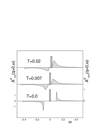
Figure 1: The boson spectral function $A^{B}({\bf q}={\bf 0},\omega)$ for three representative temperatures $T=0.02>T^{*}$ (top), $T=0.007<T^{*}$ (middle) and for the ground state superconducting phase $T=0$ (bottom). The BFM parameters are $n_{tot}=1$, $v=0.1$, $\Delta_{B}=-0.6$ (energies are expressed in units of the initial fermion bandwidth $D\equiv 1$).

Figure 1 shows the results obtained numerically for the single particle boson spectral function $A^{B}({\bf q},\omega)$ in the long wavelength limit ${\bf q}={\bf 0}$. We illustrate three distinct situations corresponding to: the normal phase above $T^{*}$ (top panel), the normal phase with the pseudogap structure present in the single particle fermion spectrum (middle panel) and the superconducting state at $T=0$ (bottom panel). In this paper we have chosen the same set of parameters as previously Domanski-01 , i.e. $\Delta_{B}=0.4$, $n_{tot}=1$, $v=0.1$ such, that the temperature at which the pseudogap begins to open up is roughly $T^{*}\sim 0.1$.

Our study of the superconducting phase (following the previous work Domanski-01 ) is based on a three-dimensional system with a BCS type of approach, as far as the fermionic subsystems is concerned, and a BE condensation approach for free bosons, as far as the bosonic subsystem is concerned. We notice, that in this phase there is a perfect separation of the coherent part (describing the long lived quasiparticles) from the incoherent part of the spectrum. Moreover: (a) the coherent peak is pinned at $\omega=0$ allowing for a macroscopic occupancy of the zero momentum state by a certain fraction $n_{cond}^{B}$ of the BE condensed bosons, (b) the incoherent part $A_{inc}^{B}({\bf q},\omega)$ exists only outside a energy window (equal $2v\;\sqrt{n_{cond}^{B}}$ as will be explained in section IV.D). Owing to such a behavior, the condensed bosons are not damped and they are able to establish a long range order parameter in the boson subsystem. On the other hand in the normal phase above $T^{*}$ the coherent and incoherent parts overlap with each other and consequently the boson quasiparticles are damped. This damping is caused by some very reduced remanent inter-boson interaction of the order of $v^{4}$, which arises in this renormalization procedure Domanski-01 .

The pseudogap phase (middle panel of Fig. 1) represents some intermediate situation, where we notice that the incoherent background is partly pushed away from the coherent peak. Thus the zero momentum bosons start to emerge as better and better quasiparticles upon approaching $T_{c}$ from above. Yet, the zero momentum boson state is macroscopically occupied only below $T_{c}$.

In the BFM there is a strict relation between the single particle boson and fermion pair excitation spectra (see equations (III.2,30) in the next section). By inspecting Fig. 1 (and figure 3 presented below) we conclude that zero momentum fermion pairs gradually emerge in the pseudogap phase ($T^{*}>T$). Upon lowering the temperature, the surrounding incoherent background fades away and thus effectively leads to increase of the life-time of the zero momentum bosons and fermion pairs. For $T<T_{c}$, these entities acquire an infinite life-time. Experiments, sensitive to the short lived Cooper pairs, should be able to detect their presence above $T_{c}$. This type of a precursor phenomenon was indeed observed for the HTS cuprates using the alternating magnetic fields in the terahertz frequencies regime Corson-99 . A residual Meissner effect was seen there up to nearly 25 K above the transition temperature $T_{c}$ and which is an indication that propagating fermion pairs exist there on a corresponding short time scale.

In figure 2 we compare the boson spectral function $A^{B}({\bf q},\omega)$ for several momenta $q=|{\bf q}|$ at two different temperatures: above (column on the left) and below $T^{*}$ (column on the right). We notice that at finite momenta there is is a qualitative difference between these spectra. At temperatures $T>T^{*}$ the coherent peak is always covered by the incoherent background signaling that these components are convoluted with each other. On the contrary, at temperatures below $T^{*}$, the coherent boson peak separates from the incoherent states. Such a splitting-off is very sensitive to moderate temperature changes and, for example at $T=0.004$, occurs above a critical momentum $q_{crit}\simeq 0.01\times\pi/a$. This critical value decreases with decreasing temperature and finally $q_{crit}(T_{c})\rightarrow 0$. We thus see that for momenta $q>q_{crit}(T)$ the coherent boson states, representing the long lived propagating modes are not scattered by the incoherent background.

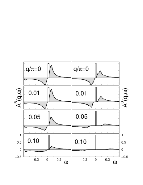
Figure 2: Variation of the boson spectral function $A^{B}({\bf q},\omega)$ with respect to changing momentum $q$ at high temperature $T=0.02>T^{*}$ (panels on the l.h.s.) and low temperature $T=0.004$ (panels on the r.h.s.) corresponding to the pseudogap region $T^{*}>T>T_{c}$. The lattice constant is taken as a unit $a\equiv 1$.

Our finding, that under certain conditions the boson peak becomes well separated from the background of incoherent states $A^{B}_{inc}({\bf q},\omega)$, means that in the pseudogap regime ($T^{*}>T>T_{c}$) the finite momentum bosons are well defined quasi-particles with infinite life-time. Since bosons are closely related to the fermion Cooper pairs, we further conclude that for $q>q_{crit}(T)$ there exist infinite life-time cooperons above the transition temperature $T_{c}$. According to the Heisenberg principle, experiments measuring the pair-pair correlations restricted to spatial distance smaller than $\Delta x\sim 1/q_{crit}(T)$ (of the order of several lattice constants) should be able to detect such fermion pairs. And indeed, such long-lived ”moving” fermion pairs were observed up to very high temperatures above $T_{c}$ by applying a thermal gradient and measuring the Nernst coefficient in underdoped HTS materials Ong-00 .

III.2 Flow of the cooperon operators

We have seen in the previous section that the boson operators get mixed for $l>0$ with the fermion pair operators. Now we expect that, in turn, also the latter become convoluted with $b_{\bf q}$ during such a transformation. By calculating the initial ($l$$=$$0$) derivative of the cooperon operators $S_{\bf q}^{-}\equiv N^{-1}\sum_{\bf k}c_{{\bf k}\downarrow}c_{{\bf q}-{\bf k}\uparrow}$ we obtain

$$\frac{dS_{\bf q}^{-}}{dl}=-\frac{1}{\sqrt{N}}\sum_{\bf k}\alpha_{{\bf k},{\bf q}-{\bf k}}(0)f_{{\bf k},{\bf q}-{\bf k}}\;b_{\bf q}.$$ (23)

In accordance with the previous substitution (17) we propose the following Ansatz

$$S_{\bf q}^{-}(l)=\frac{1}{\sqrt{N}}\sum_{\bf k}{\cal{M}}_{{\bf k},{\bf q}}(l)c_{{\bf k}\downarrow}c_{{\bf q}-{\bf k}\uparrow}+{\cal{N}}_{\bf q}(l)b_{\bf q}$$ (24)

with the initial conditions ${\cal{M}}_{{\bf q},{\bf k}}(0)=1$ and ${\cal{N}}_{\bf q}(0)=0$. After substituting the expression (24) into (10) we get

$$\frac{d{\cal{M}}_{{\bf q},{\bf k}}(l)}{dl} = \alpha_{{\bf k},{\bf q}-{\bf k}}(l){\cal{N}}_{\bf q}(l)$$ (25)

$$\frac{d{\cal{N}}_{\bf q}(l)}{dl} = -\frac{1}{N}\sum_{\bf k}\alpha_{{\bf k},{\bf q}-{\bf k}}(l)f_{{\bf k},{\bf q}-{\bf k}}\;{\cal{M}}_{{\bf q},{\bf k}}(l)$$ (26)

We recognize that the flow equations (25, 26) for the unknown coefficients $M_{{\bf q},{\bf k}}(l)$ and $N_{\bf q}(l)$ have a structure identical to that given by (18,19). There is only a difference in the initial conditions which in this case lead to the following invariance

$$|{\cal{N}}_{\bf q}(l)|^{2}+\frac{1}{N}\sum_{\bf k}f_{{\bf k},{\bf q}-{\bf k}}|{\cal{M}}_{{\bf q},{\bf k}}(l)|^{2}=1-n_{F}.$$ (27)

In the r.h.s. of equation (27) we made use of the property that $N^{-1}\sum_{\bf k}f_{{\bf k},{\bf q}-{\bf k}}=1-n_{F}$, where $n_{F}=N^{-1}\sum_{{\bf k},\sigma}n_{{\bf k}\sigma}^{F}$ denotes the total concentration of fermions. Equation (27) assures the proper statistical relation between the cooperon operators $\left[S_{\bf q}^{-}(l),S_{\bf q}^{+}(l)\right]=N^{-1}\sum_{\bf k}(1-c_{{\bf q}-{\bf k}\uparrow}^{\dagger}c_{{\bf q}-{\bf k}\uparrow}-c_{{\bf k}\downarrow}^{\dagger}c_{{\bf k}\downarrow})$, which can be approximated by the c-number $\simeq 1-n_{F}$.

With the Ansatz (24) and using its hermitian conjugate $S_{\bf q}^{+}(l)$ we can now determine the two particle fermion Green’s function $G^{pair}({\bf k},\tau)$ defined in (15). The corresponding spectral function (11) becomes

$$A^{pair}({\bf q},\omega)=|{\cal{N}}_{\bf q}(\infty)|^{2}\delta\left(\omega-\tilde{E}_{\bf q}\right)$$ (28)

$$+\frac{1}{N}\sum_{\bf k}f_{{\bf k},{\bf q}-{\bf k}}|{\cal{M}}_{{\bf q},{\bf k}}(\infty)|^{2}\delta\left(\omega-\tilde{\varepsilon}_{\bf k}-\tilde{\varepsilon}_{{\bf q}-{\bf k}}\right).$$

The cooperon spectral function turns out to have a structure similar to $A^{B}({\bf q},\omega)$, expressed in (III.1). This is a general feature of the BFM which, in particular, implies that bosons BE condense simultaneously with the fermion pairs driven to superconductivity Kostyrko-96 .

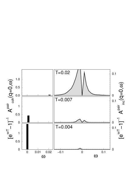
Figure 3: The cooperons’ occupancy $\left[\mbox{exp}(\omega/k_{B}T)-1\right]^{-1}\times A^{pair}({\bf q},\omega)$ of the zero momentum coherent (left h.s. panel) and incoherent (right h.s. panel) states for three representative temperatures: $T=0.02$ (above $T^{*}$) and $T=0.007$, $0.004$ (below $T^{*}$). With lowering temperature the incoherent fermion pairs are converted into the coherent quasi-particles.

We limit our quantitative discussion of the cooperon spectral function (28) by only presenting in Fig. 3 a distribution of the occupied coherent and incoherent states in the long wavelength limit ${\bf q}={\bf 0}$. Above $T^{*}$ almost all the cooperons exist as incoherent objects. Upon decreasing the temperature more and more incoherent pairs are converted into coherent ones. Yet, because of their overlap with the incoherent background the Cooper pairs can propagate only on a short time scale.

The fact that the overall structure of the cooperon spectral function $A^{pair}({\bf q},\omega)$ is to great extent similar to the single particle boson function $A^{B}({\bf q},\omega)$ is not surprising. Using for instance the equation of motion technique for the Green’s functions one can prove the following important identity Kostyrko-96

$$G^{B}({\bf q},\omega) = G^{B}_{0}({\bf q},\omega)+$$

$$+ v^{2}\;G^{B}_{0}({\bf q},\omega)G^{pair}({\bf q},\omega)G^{B}_{0}({\bf q},\omega),$$

where $G^{B}_{0}({\bf q},\omega)=\left[\omega-\Delta_{B}+2\mu\right]^{-1}$ denotes the single particle boson Green’s function of the non-interacting system. Both Green’s functions $G^{pair}({\bf q},\omega)$ and $G^{B}({\bf q},\omega)$ have thus common poles and their spectral functions are correspondingly related via

$$A^{pair}({\bf q},\omega)=\frac{\left(\omega-\Delta_{B}+2\mu\right)^{2}}{v^{2}}\;A^{B}({\bf q},\omega).$$ (30)

For ${\bf q}={\bf 0}$, when the single particle boson Green’s function develops a pole at $\omega=0$, the two particle cooperon propagator is characterized by the same pole - although with a different weight. This automatically causes a divergence of the static pair susceptibility and via the Thouless criterion leads to the phase transition into a superconducting state.

We want to stress that all our conclusions concerning the evolution of the boson spectral function $A^{B}({\bf q},\omega)$ are also valid for $A^{pair}({\bf q},\omega)$. In particular, we emphasize, that in the pseudogap region $T^{*}>T>T_{c}$ there exist fermion Cooper pairs. Fermion pairs with total zero momentum are convoluted with incoherent background states and therefore their life time is finite. They can be detected experimentally only via some short time impulses. On the other hand, long-lived fermion pairs can safely exist if their total momentum exceeds the critical value $q>q_{crit}(T)$. In this case correlations between the fermion pairs can possibly extend over the spatial distance up to $\Delta x\sim 1/q_{crit}$. A possibility to observe correlations between the fermion pairs above $T_{c}$ over a short spatial and temporal scale had been previously suggested by Tchernyshyov Tchernyshyov-97 .

IV Fermions

IV.1 Flow of the single particle fermion operators

Some aspects of the effective single particle fermion excitations were already discussed in our recent Letter PRL-03 . We focused our discussion there on the single particle fermion spectrum for a narrow region around the Fermi surface ${\bf k}\sim{\bf k}_{F}$. We have shown that the pseudogap is accompanied by an appearance of the Bogoliubov-like branches. The shadow part of these Bogoliubov modes is visible above $T_{c}$ as a broad structure which narrows upon approaching $T_{c}$. Below $T_{c}$ both branches become infinitely narrow, signaling that bogoliubons become then the true, long-lived quasi-particles. This result is herewith confirmed from our present direct study of the boson and fermion pair spectra, illustrated in figures 1-3.

In this section we would like to present a detailed derivation of the diagonal and off-diagonal parts (in a Nambu spinor representation) of the single particle fermion Green’s function. We will discuss the diagonal and off-diagonal parts studying their structure over the whole Brillouin zone above and below $T_{c}$.

Let us briefly recapitulate the main properties of the fermion operators $c_{{\bf k}\sigma}^{\dagger}$ and $c_{{\bf k}\sigma}$ resulting from the continuous canonical transformation. At the initial step (i.e. for $l=0$) their derivatives read

$$\mp\frac{dc_{{\bf k}\sigma}}{dl} = \alpha_{-{\bf k},{\bf k}}(0)\frac{b_{\bf 0}}{\sqrt{N}}\;c_{-{\bf k},-\sigma}^{\dagger}$$ (31)

$$+ \frac{1}{\sqrt{N}}\sum_{{\bf q}\neq{\bf 0}}\alpha_{{\bf q}-{\bf k},{\bf k}}(0)b_{\bf q}c_{{\bf q}-{\bf k},-\sigma}^{\dagger}$$

where the negative sign corresponds to $\sigma=\uparrow$ and the positive sign to $\sigma=\downarrow$. The first term on the r.h.s. of (31) shows that the fermion particles get mixed with the fermion holes. The last term in (31) corresponds to scattering of fermions on bosons with finite momentum.

As a consequence of (31) we imposed the following parametrization of the $l$-dependent fermion operators

$$c_{{\bf k}\uparrow}(l)={\cal{P}}_{\bf k}(l)\;c_{{\bf k}\uparrow}+{\cal{R}}_{\bf k}(l)\;c_{-{\bf k}\downarrow}^{\dagger}$$

$$+ \;\frac{1}{\sqrt{N}}\sum_{{\bf q}\neq{\bf 0}}\left[p_{{\bf k},{\bf q}}(l)\;b_{\bf q}^{\dagger}c_{{\bf q}+{\bf k}\uparrow}+r_{{\bf k},{\bf q}}(l)\;b_{\bf q}c_{{\bf q}-{\bf k}\downarrow}^{\dagger}\right]$$

$$c_{-{\bf k}\downarrow}^{\dagger}(l)=-\;{\cal{R}}_{\bf k}^{*}(l)\;c_{{\bf k}\uparrow}+{\cal{P}}_{\bf k}^{*}(l)\;c_{-{\bf k}\downarrow}^{\dagger}$$

$$- \;\frac{1}{\sqrt{N}}\sum_{{\bf q}\neq{\bf 0}}\left[r_{{\bf k},{\bf q}}^{*}(l)\;b_{\bf q}^{\dagger}c_{{\bf q}+{\bf k}\uparrow}-p_{{\bf k},{\bf q}}^{*}(l)\;b_{\bf q}c_{{\bf q}-{\bf k}\downarrow}^{\dagger}\right].$$

In this case, the initial conditions read ${\cal{P}}_{\bf k}(0)=1$, ${\cal{R}}_{\bf k}(0)=0$ and $p_{{\bf k},{\bf q}}(0)=0$, $r_{{\bf k},{\bf q}}(0)=0$. As we have stated previously PRL-03 , equations (IV.1,IV.1) generalize the standard Bogoliubov-Valatin transformation Bogol-Valatin in a twofold way: (a) the initial particle and hole operators are transformed into cooperons (bogoliubons) through a continuous transformation, (b) the scattering of finite momentum Cooper pairs is additionally taken into account via terms containing the coefficients $p_{{\bf k},{\bf q}}(l)$ and $r_{{\bf k},{\bf q}}(l)$.

¿From (10) one can derive the set of differential equations for a determination of the $l$-dependent coefficients appearing in (IV.1,IV.1). Because of their importance, for our further discussion we repeat them here again PRL-03

$$\frac{d{\cal{P}}_{\bf k}(l)}{dl} = \sqrt{n_{cond}^{B}}\;\alpha_{-{\bf k},{\bf k}}(l)\;{\cal{R}}_{\bf k}(l),$$

$$+ \frac{1}{N}\sum_{{\bf q}\neq{\bf 0}}\alpha_{{\bf q}-{\bf k},{\bf k}}(l)\left(n_{\bf q}^{B}+n_{{\bf q}-{\bf k}\downarrow}^{F}\right)r_{{\bf k},{\bf q}}(l)$$

$$\frac{d{\cal{R}}_{\bf k}(l)}{dl} = -\;\sqrt{n_{cond}^{B}}\;\alpha_{{\bf k},-{\bf k}}(l)\;{\cal{P}}_{\bf k}(l),$$

$$- \frac{1}{N}\sum_{{\bf q}\neq{\bf 0}}\alpha_{-{\bf k},{\bf q}+{\bf k}}(l)\left(n_{\bf q}^{B}+n_{{\bf q}+{\bf k}\uparrow}^{F}\right)p_{{\bf k},{\bf q}}(l)$$

$$\frac{dp_{{\bf k},{\bf q}}(l)}{dl} = \alpha_{-{\bf k},{\bf q}+{\bf k}}(l)\;{\cal{R}}_{\bf k}(l),$$ (36)

$$\frac{dr_{{\bf k},{\bf q}}(l)}{dl} = -\;\alpha_{{\bf k},{\bf q}-{\bf k}}(l){\cal{P}}_{\bf k}(l).$$ (37)

$n_{cond}^{B}$ denotes the concentration of the BE condensed bosons and $n_{\bf q}^{B}\equiv\langle b_{\bf q}^{\dagger}b_{\bf q}\rangle$ is the distribution of finite momentum ${\bf q}\neq{\bf 0}$ bosons. Equations (IV.1-37) properly preserve the fermionic anti-commutation relations $\left\{c_{{\bf k}\uparrow}(l),c_{{\bf p}\uparrow}(l)^{\dagger}\right\}=\delta_{{\bf k},{\bf p}}$ and $\left\{c_{{\bf k}\sigma}(l),c_{{\bf p}\sigma^{\prime}}(l)\right\}=0$.

The single particle fermion Green’s function can be easily obtained in the limit $l\rightarrow\infty$ when the fermions are no longer coupled to the boson subsystem $v_{{\bf k},{\bf p}}(\infty)=0$. We have shown previously PRL-03 that the diagonal part reads

$$A_{d}^{F}({\bf k},\omega)$$

$$= |{\cal{P}}_{\bf k}(\infty)|^{2}\delta\left(\omega-\tilde{\varepsilon}_{\bf k}\right)+|{\cal{R}}_{\bf k}(\infty)|^{2}\delta\left(\omega+\tilde{\varepsilon}_{-{\bf k}}\right)$$

$$+ \frac{1}{N}\sum_{{\bf q}\neq{\bf 0}}\left(n_{\bf q}^{B}+n_{{\bf q}+{\bf k}\uparrow}^{F}\right)|p_{{\bf k},{\bf q}}(\infty)|^{2}\delta(\omega+\tilde{E}_{\bf q}-\tilde{\varepsilon}_{{\bf q}+{\bf k}})$$

$$+ \frac{1}{N}\sum_{{\bf q}\neq{\bf 0}}\left(n_{\bf q}^{B}+n_{{\bf q}-{\bf k}\downarrow}^{F}\right)|r_{{\bf k},{\bf q}}(\infty)|^{2}\delta(\omega-\tilde{E}_{\bf q}+\tilde{\varepsilon}_{{\bf q}-{\bf k}}),$$

and that it correctly satisfies the sum rule $\int d\omega A_{d}^{F}({\bf k},\omega)=1$. The spectral function (IV.1) consists of the delta function peaks which represent the long-lived quasi-particles and a remaining incoherent background $A_{d,\,inc}^{F}({\bf k},\omega)$ of the damped fermion states. It should be mentioned that a similar result was obtained by M. Fisher and coworkers Lannert-01 for the 2 dimensional Hubbard model with a fractionalized structure. Those authors considered the spinon and chargon degrees of freedom coupled to a Z₂ gauge field. At low temperatures the spinons and chargons are confined. Their deconfinement becomes possible at finite temperatures by overcoming the gap of ”vison” excitations. From an analysis of the low energy excitations those authors derived the effective spectral function for physical electrons which took exactly the same form as our result (IV.1). Apart from a common structure of the spectral functions, the remaining discussion and interpretation for both models is different.

The spectral function for the off-diagonal part of the fermion Green’s function $\left<\left<c_{{\bf k}\uparrow}(\tau);c_{-{\bf k}\downarrow}\right>\right>$ becomes

$$A_{od}^{F}({\bf k},\omega)={\cal{P}}_{\bf k}(\infty){\cal{R}}_{\bf k}(\infty)\left[\delta\left(\omega+\tilde{\varepsilon}_{\bf k}\right)-\delta\left(\omega-\tilde{\varepsilon}_{\bf k}\right)\right]$$

$$+\frac{1}{N}\sum_{{\bf q}\neq{\bf 0}}p_{{\bf k},{\bf q}}(\infty)r_{{\bf k},{\bf q}}(\infty)\left\{\delta(\omega+\tilde{E}_{\bf q}-\tilde{\varepsilon}_{{\bf q}+{\bf k}})\right.$$ (39)

$$\left.\times\left[n_{\bf q}^{B}+n_{{\bf q}+{\bf k}\uparrow}^{F}\right]-\delta(\omega-\tilde{E}_{\bf q}+\tilde{\varepsilon}_{{\bf q}-{\bf k}})\left[n_{\bf q}^{B}+n_{{\bf q}-{\bf k}\downarrow}^{F}\right]\right\}$$

which conserves the sum rule $\int d\omega A^{F}_{od}({\bf k},\omega)=0$. This function consists also of the delta peaks and some fraction distributed over a wide energy region. In what follows below we shall study the properties of the diagonal and off-diagonal spectral functions in various temperature regions.

IV.2 The normal phase spectrum

Above the critical temperature $T_{c}$ there is no boson condensate $n_{cond}^{B}=0$ and in such a case the flow equations (IV.1,37) become decoupled from (IV.1,36). Consequently the coefficients ${\cal{R}}_{\bf k}(l)$ and $p_{{\bf k},{\bf q}}(l)$ do not change their initial zero values, i.e.

$${\cal{R}}_{\bf k}(l)=0,\hskip 28.45274ptp_{{\bf k},{\bf q}}(l)=0.$$ (40)

This property (40) has a strong influence on both fermion spectral functions. The off-diagonal part identically vanishes $A^{F}_{od}({\bf k},\omega)=0$ what implies that above $T_{c}$ there exists no long range order parameter in the fermion system.

The spectral function of the diagonal part is described by

$$A_{d}^{F}({\bf k},\omega)=|{\cal{P}}_{\bf k}(\infty)|^{2}\delta\left(\omega-\tilde{\varepsilon}_{\bf k}\right)$$

$$+ \frac{1}{N}\sum_{{\bf q}\neq{\bf 0}}\left(n_{\bf q}^{B}+n_{{\bf q}-{\bf k}\downarrow}^{F}\right)|r_{{\bf k},{\bf q}}(\infty)|^{2}\delta(\omega-\tilde{E}_{\bf q}+\tilde{\varepsilon}_{{\bf q}-{\bf k}}).$$

We thus have just one branch of long-lived fermion states described by the dispersion $\tilde{\varepsilon}_{\bf k}$ and which can be obtained from the renormalization scheme discussed by us in Ref. Domanski-01 . For a clear understanding of the resulting low energy physics we show the temperature evolution of this quantity in figure 4 together with the corresponding spectral weight $|{\cal{P}}_{\bf k}(\infty)|^{2}$. Below a certain characteristic temperature $T^{*}$ (in this case $T^{*}\sim 0.1$) we observe a tendency to form the pseudogap. Simultaneously there occurs a partial transfer of the spectral weight from the quasi-particle peak to the incoherent background states (see the bottom panel of Fig. 4).

Figure 4: Dispersion of the effective single particle fermion energy $\tilde{\varepsilon}_{\bf k}$ for several temperatures (upper panel) and spectral weights of the coherent and incoherent parts for $T=0.02$ and $0.004$ (bottom panel). Momentum is expressed in units $1/a$.

Such a transfer of the spectral weight is responsible for the appearance of the Bogoliubov shadow band, as shown from the selfconsistent numerical calculations in Ref. PRL-03 . We will prove this result here analytically. When the temperature approaches $T_{c}$ from above, bosons tend to occupy macroscopically the lowest lying states of energies $\tilde{E}_{\bf q}\simeq 0$. These states are spread over the momentum region $|{\bf q}|\leq\Lambda$ with the cutoff $\Lambda$ being a fraction of the inverse lattice spacing $a^{-1}$. Since the boson occupancy of low momenta is much larger than the fermion population $n^{F}_{{\bf q}-{\bf k}}$ we can simplify (IV.2) to the following form

$$A_{d}^{F}({\bf k},\omega) \simeq |{\cal{P}}_{\bf k}(\infty)|^{2}\;\delta\left(\omega-\tilde{\varepsilon}_{\bf k}\right)$$ (42)

$$+ |r_{{\bf k},{\bf q}\simeq{\bf 0}}(\infty)|^{2}\sum_{|{\bf q}|\leq\Lambda}\frac{n^{B}_{\bf q}}{N}\;\delta(\omega+\tilde{\varepsilon}_{-{\bf k}}-\tilde{E}_{\bf q})$$

$$+ A^{F}_{d,rigid}({\bf k},\omega),$$

where $A^{F}_{d,rigid}({\bf k},\omega)=N^{-1}\sum_{|{\bf q}|>\Lambda}n_{{\bf q}-{\bf k}\downarrow}^{F}|r_{{\bf k},{\bf q}}(\infty)|^{2}$ $\times\delta(\omega+\tilde{\varepsilon}_{{\bf q}-{\bf k}}-\tilde{E}_{\bf q})$ represents a rigid background which is weakly sensitive to varying the temperature. Integrating over the small momentum boson states (whose energies are negligible $\tilde{E}_{\bf q}\simeq 0$) we obtain a partly broadened peak with its maximum occurring at $\omega=-\tilde{\varepsilon}_{\bf k}$. This additional branch of fermion excitations can well be fitted by the Lorentzian shape

$$\sum_{|{\bf q}|\leq\Lambda}\frac{n^{B}_{\bf q}}{N}\;\delta(\omega+\tilde{\varepsilon}_{-{\bf k}}-\tilde{E}_{\bf q})\simeq\frac{n^{B}}{\pi}\;\frac{\Gamma_{\bf k}}{(\omega+\tilde{\varepsilon}_{-{\bf k}})^{2}+\Gamma_{\bf k}^{2}}$$ (43)

with $n^{B}$ being the concentration of bosons. For $T<T_{c}$ (43) shrinks to $\Gamma\rightarrow 0$. Similar Bogoliubov shadow bands were also indicated for the normal phase of the $U<0$ Hubbard model using the Quantum Monte Carlo studies Zurich_group and the conserving diagrammatic treatment of Tremblay and coworkers Tremblay-97 . In our case the Bogoliubov-like branches are characterized by the pseudogap dispersion $\pm\tilde{\varepsilon}_{\bf k}$ shown here in figure 4. Above $T_{c}$ the shadow branch (corresponding to $-$ sign) is broad as discussed in our Letter PRL-03 .

Far away from the Fermi surface the renormalized energies are nearly equal to the bare values $\tilde{\varepsilon}_{\bf k}=\varepsilon_{\bf k}-\mu$. The long-lived quasi-particle contains however only part of the spectral weight, i.e., $|{\cal{P}}_{\bf k}(\infty)|^{2}<1$. In figure 5 we illustrate the coherent and incoherent contributions of the single particle fermion spectral function (IV.2) in a large part of the Brillouin zone. The damped fermion states are spread over the large energy regime $\omega$, they exist even for momenta quite distant from $k_{F}$. This result agrees well with the previous studies based on selfconsistent perturbative theory (see the third reference of Ranninger_etal ). The presence of the substantial incoherent background states might possibly be related to the experimental signal observed in the ARPES measurements for the HTS compounds ARPES-exp .

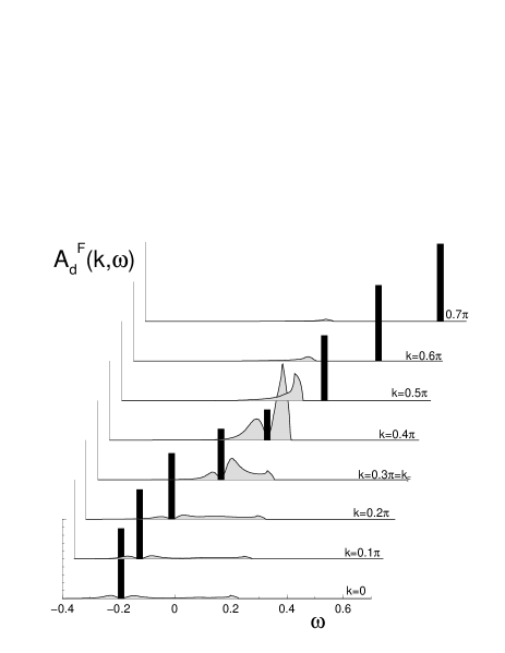
Figure 5: Diagonal part of the single particle fermion spectral function (IV.2) for a large part of the Brillouin zone at $T=0.007$. Vertical bars represent the coherent part $A_{d,coh}^{F}({\bf k},\omega)$ while the shaded area corresponds to $A_{d,inc}^{F}({\bf k},\omega)$. Besides only a close vicinity of the Fermi surface (consult (43) or see the figure 1 in PRL-03 ) this spectral function is rather weakly affected by temperature.

IV.3 The long-lived quasiparticles below $T_{c}$

Below the critical temperature $T_{c}$ there exists a finite amount of the BE condensed bosons $n_{cond}^{B}\neq 0$. This has important effects on the fermionic spectrum. Using the flow equation method we have shown analytically Domanski-01 that $\tilde{\varepsilon}_{{\bf k}}=\mbox{sgn}(\varepsilon_{\bf k}-\mu)\sqrt{(\varepsilon_{\bf k}-\mu)^{2}+v^{2}n_{cond}^{B}}$. In the superconducting phase the effective dispersion is thus characterized by the true gap $\Delta_{sc}(T)=v\sqrt{n_{cond}^{B}(T)}$.

For a finite condensate fraction $n_{cond}^{B}$, we can see from equations (IV.1,36) that the coefficients ${\cal{R}}_{\bf k}$ and $p_{{\bf k},{\bf q}}$ become finite too. The long-lived fermion excitations are then represented by the two sharp Bogoliubov branches

$$A_{d,coh}^{F}({\bf k},\omega) = |{\cal{P}}_{\bf k}(\infty)|^{2}\;\delta\left(\omega-\tilde{\varepsilon}_{\bf k}\right)$$ (44)

$$+ |{\cal{R}}_{\bf k}(\infty)|^{2}\;\delta\left(\omega+\tilde{\varepsilon}_{{\bf k}}\right).$$

Similarly, the coherent part of the off-diagonal spectral function (IV.1) reads

$$A^{F}_{od,coh}({\bf k},\omega) = {\cal{P}}_{\bf k}(\infty){\cal{R}}_{\bf k}(\infty)$$ (45)

$$\times \left[\delta\left(\omega+\tilde{\varepsilon}_{\bf k}\right)-\delta\left(\omega-\tilde{\varepsilon}_{\bf k}\right)\right].$$

Equations (44,45) resemble the BCS-type results which usually appear in the mean field studies of this model Micnas_etal ; Lee_etal ; Ranninger_etal . Let us stress that in distinction to these we obtain here the total spectral weight engaged in the coherent parts to be PRL-03

$$|{\cal{P}}_{\bf k}(\infty)|^{2}+|{\cal{R}}_{\bf k}(\infty)|^{2}<1.$$ (46)

The rest of the weight is redistributed over the damped fermionic states. This will be discussed separately in the next section.

In order to show the correspondence of our present analysis to the previous results for this BF model we prove in Appendix A, that upon neglecting the incoherent background states of (IV.1,IV.1) one exactly obtains the usual BCS coherence factors

$$|{\cal{P}}_{\bf k}(\infty)|^{2}=\frac{1}{2}\left(1+\frac{|\varepsilon_{\bf k}-\mu|}{\xi_{\bf k}^{MF}}\right) = 1-|{\cal{R}}_{\bf k}(\infty)|^{2},$$ (47)

$${\cal{P}}_{\bf k}(\infty)\;{\cal{R}}_{\bf k}(\infty) = -\;\frac{v\sqrt{n_{cond}^{B}}}{2\xi_{\bf k}^{MF}},$$ (48)

where $\xi_{\bf k}^{MF}=\sqrt{(\varepsilon_{\bf k}-\mu)^{2}+\Delta_{sc}^{2}}$. By neglecting the incoherent parts, the flow equation procedure reproduces exactly the standard mean field equations Micnas_etal ; Lee_etal ; Ranninger_etal

$$\langle c_{{\bf k}\uparrow}^{\dagger}c_{{\bf k}\uparrow}\rangle = \frac{1}{2}\left[1-\frac{\varepsilon_{\bf k}-\mu}{\xi_{\bf k}^{MF}}\;\mbox{tgh}\left(\frac{\xi_{\bf k}^{MF}}{2k_{B}T}\right)\right],$$ (49)

$$\langle c_{-{\bf k}\downarrow}c_{{\bf k}\uparrow}\rangle = -\;\frac{v\;n_{cond}^{B}}{2\xi_{\bf k}^{MF}}\;\mbox{tgh}\left(\frac{\xi_{\bf k}^{MF}}{2k_{B}T}\right).$$ (50)

We shall generalize these equations (49, 50) in the next section, taking into account the contribution from the damped fermion states.

IV.4 Damped quasi-particles below $T_{c}$

The finite life-time (damped) states do participate in the fermionic excitation spectrum both above $T_{c}$ as well as below of it. Nevertheless their presence does not spoil a long range coherent behavior between the fermion pairs which is necessary for superconductivity to occur. In chapter III we saw that boson as well as the fermion pair spectra are characterized below $T_{c}$ by long-lived collective modes with $\tilde{E}_{\bf q}\propto|{\bf q}|$ Domanski-01 which becomes separated from the surrounding background of incoherent states by the gap $2\Delta_{sc}$. We show below that in the single particle excitation spectrum the incoherent states can exist only outside the gap $\Delta_{sc}$ around the Fermi energy.

The contribution from the damped fermionic states is described by the following part of the spectral function (IV.1)

$$A_{d,inc}^{F}({\bf k},\omega)=A_{d}^{F}({\bf k},\omega)-A_{d,coh}^{F}({\bf k},\omega)$$ (51)

$$= \frac{1}{N}\sum_{{\bf q}\neq{\bf 0}}\left[\left(n_{\bf q}^{B}+n_{{\bf q}+{\bf k}\uparrow}^{F}\right)|p_{{\bf k},{\bf q}}(\infty)|^{2}\delta(\omega+\tilde{E}_{\bf q}-\tilde{\varepsilon}_{{\bf q}+{\bf k}})\right.$$

$$+ \left.\left(n_{\bf q}^{B}+n_{{\bf q}-{\bf k}\downarrow}^{F}\right)|r_{{\bf k},{\bf q}}(\infty)|^{2}\delta(\omega-\tilde{E}_{\bf q}+\tilde{\varepsilon}_{{\bf q}-{\bf k}})\right]$$

and similarly in case of the off-diagonal function (IV.1)

$$A_{od,inc}^{F}({\bf k},\omega)=-\;\frac{1}{N}\sum_{{\bf q}\neq{\bf 0}}p_{{\bf k},{\bf q}}(\infty)r_{{\bf k},{\bf q}}(\infty)$$

$$\times\left[\left(n_{\bf q}^{B}+n_{{\bf q}+{\bf k}\uparrow}^{F}\right)\delta(\omega+\tilde{E}_{\bf q}-\tilde{\varepsilon}_{{\bf q}+{\bf k}})\right.$$

$$\left.-\left(n_{\bf q}^{B}+n_{{\bf q}-{\bf k}\downarrow}^{F}\right)\delta(\omega-\tilde{E}_{\bf q}+\tilde{\varepsilon}_{{\bf q}-{\bf k}})\right].$$ (52)

It is instructive to consider first the incoherent spectral functions (51,52) for the ground state $T=0$. Finite momenta bosons have $\tilde{E}_{{\bf q}\neq{\bf 0}}>0$, such that all bosons are condensed at $T=0$ and we can put $n_{\bf q}^{B}=0$ for any ${\bf q}\neq{\bf 0}$. On the other hand, fermions occupy only the states below the Fermi surface, i.e. $n_{{\bf k}\sigma}^{F}=\theta(-\tilde{\varepsilon}_{\bf k})n_{{\bf k}\sigma}^{F}$. Therefore, the first term on the r.h.s. of (51) gives rise to the appearance of the incoherent fermion states at negative energies. It can be written as

$$A_{d,inc}^{F}({\bf k},\omega<0)$$

$$= \frac{1}{N}\sum_{\tilde{\varepsilon}_{{\bf q}+{\bf k}}<0}n^{F}_{{\bf q}+{\bf k}\uparrow}|p_{{\bf k},{\bf q}}(\infty)|^{2}\delta\left[\omega+\left(\tilde{E}_{\bf q}+|\tilde{\varepsilon}_{{\bf q}+{\bf k}}|\right)\right].$$

Similarly, the last term in (51), which corresponds to incoherent states at positive energies, becomes

$$A_{d,inc}^{F}({\bf k},\omega>0)$$

$$= \frac{1}{N}\sum_{\tilde{\varepsilon}_{{\bf q}-{\bf k}}<0}n^{F}_{{\bf q}-{\bf k}\downarrow}|r_{{\bf k},{\bf q}}(\infty)|^{2}\delta\left[\omega-\left(\tilde{E}_{\bf q}+|\tilde{\varepsilon}_{{\bf q}-{\bf k}}|\right)\right].$$

The off-diagonal spectral function (52) can be derived in the same manner. From inspecting their structure we notice that:

• no damped fermion states are allowed to occur within the superconducting energy gap window $|\omega|\leq\Delta_{sc}$ because $|\tilde{\varepsilon}_{{\bf q}\pm{\bf k}}|\geq\Delta_{sc}$,

• even outside the superconducting gap, in a close vicinity of the coherence peaks (44) there is a partial suppression of the damped fermion states due to finite $\tilde{E}_{\bf q}$ in equations (IV.4,IV.4). As shown in our earlier studies Ranninger_etal ; Domanski-01 the width of such a boson band is rather small and of the order $v^{2}/D$.

The incoherent fermion states can thus be formed only outside the superconducting gap $|\omega|>\Delta_{sc}$ and yet they are strongly suppressed over some small energy region (of the order $v^{2}/D$ from the coherence peaks).

To summarize our results of the last two sections , we conclude that the single particle fermion spectral function (IV.1) is characterized in the superconducting phase by: (a) the presence of narrow quasi-particle peaks at $\omega=\pm\sqrt{(\varepsilon_{\bf k}-\mu)^{2}+\Delta_{sc}^{2}}$, (b) the partial suppression of the fermionic states very close to the coherence peaks, giving rise to the appearance of the dip-like structure, (c) the existence of a broad incoherent background spectrum with its flat maximum (hump) situated fairly away from the Fermi energy. Upon increasing the temperature we expect the dip-like structure to be gradually filled in via absorbing part of the spectral weight from the coherent Bogoliubov peaks. Our expectation is motivated here by the fact that the spectral weights $|{\cal{P}}_{\bf k}(\infty)|^{2}$, $|{\cal{R}}_{\bf k}(\infty)|^{2}$ of the coherent peaks are very sensitive to temperature because of $n^{B}_{cond}(T)$ appearing in their flow equations (IV.1,IV.1).

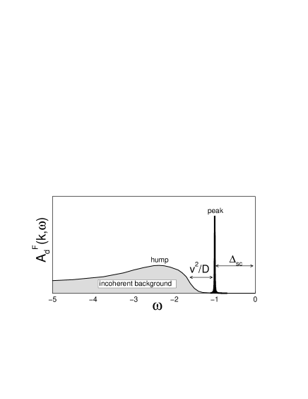
Figure 6: Schematic view of the single particle fermion spectral function $A_{d}^{F}({\bf k}_{F},\omega<0)$ in the ground state of the boson fermion model. Energy $\omega$ is expressed in units of the superconducting gap which is roughly scaled via $\Delta_{sc}\simeq v\sqrt{n^{B}_{cond}}$.

Our theoretical prediction concerning the single particle spectrum of the superconducting phase is in qualitative agreement with the experimental data known for the high $T_{c}$ underdoped cuprates. The direct photoemission spectroscopy probes the occupied spectrum $A^{F}({\bf k},\omega)\times\left[1+\mbox{exp}\left(\omega/k_{B}T\right)\right]^{-1}$. Photoemission measurements indeed revealed the appearance of such peak - dip - hump structure ARPES-exp . This issue has been so far interpreted in terms of the boson resonant mode to which the single particle excitations are coupled. Several candidates have been proposed in the literature for such boson modes Schrieffer ; Chubukov ; Eschrig . The BF model (1) is an alternative scenario, where bosons represent nearly localized electron pairs.

Concluding this discussion on the coherent and incoherent single particle spectra, let us stress that the expectation values for the particle distribution $n^{F}_{\bf k\sigma}$ at arbitrary temperature can be obtained by integrating over the expression (IV.1) after having been multiplied by the Fermi Dirac function $f(x)=\left(1+e^{x/k_{B}T}\right)^{-1}$, i.e.

$$n^{F}_{{\bf k}\sigma}=\int_{-\infty}^{\infty}d\omega\;A_{d}^{F}({\bf k},\omega)\;f(\omega).$$ (55)

Similarly, the order parameter determined via (IV.1) is given by

$$\langle c_{-{\bf k}\downarrow}c_{{\bf k}\uparrow}\rangle={\cal{P}}_{\bf k}(\infty){\cal{R}}_{\bf k}(\infty)\left[1-2f(\tilde{\varepsilon}_{\bf k})\right]$$

$$+\;\frac{1}{N}\sum_{{\bf q}\neq{\bf 0}}p_{{\bf k},{\bf q}}(\infty)r_{{\bf k},{\bf q}}(\infty)\left[\left(n_{\bf q}^{B}+n_{{\bf q}+{\bf k}\uparrow}^{F}\right)\right.$$ (56)

$$\times\left.f(\tilde{\varepsilon}_{{\bf q}+{\bf k}}-\tilde{E}_{\bf q})-\left(n_{\bf q}^{B}+n_{{\bf q}-{\bf k}\downarrow}^{F}\right)f(-\tilde{\varepsilon}_{{\bf q}-{\bf k}}+\tilde{E}_{\bf q})\right].$$

which generalizes the mean field equation (50). Unfortunately, at the present stage we are not able to solve numerically these equations (55, 56) for some realistic $d>2$ system when $T_{c}>0$. We will try to address this problem in the future by applying some approximate treatment.

V Conclusions

In the present paper we studied the mutual relations between the single particle and the pair excitation spectra within the BF model (1). We investigated their interdependence occurring in the superconducting phase below the critical temperature, and in the pseudogap region above $T_{c}$. Many-Body effects were treated by means of the continuous canonical transformation Wegner-94 originating from a general framework of the renormalization group technique RG-idea .

We have earlier reported Domanski-01 that, upon approaching $T_{c}$ from above, there is a partial suppression of the single particle fermion states near the Fermi energy (pseudogap). Here, we supplement this picture by showing that the pseudogap feature is accompanied by a subsequent emergence of the fermion pair properties. Such pairs can show up in the pseudogap region as long lived entities provided that their total momentum is finite and larger than a certain $q_{crit}(T)$. For $T\rightarrow T_{c}$ the critical momentum is $q_{crit}=0$, therefore all the fermion pairs become good quasi-particles. The zero momentum fermion pairs exist above $T_{c}$ only as the damped objects because of their overlap with the incoherent background. However, upon lowering the temperature such an overlap gradually diminishes which effectively leads to increase their life-time.

Although above $T_{c}$ there exist no off-diagonal long range order (ODLRO) we predict nevertheless the possibility to observe some ordering on a restricted spatial and temporal scale. Experiments using terahertz frequencies Corson-99 did indeed confirm the existence of preformed pairs in the underdoped HTS materials up to 25 degrees above $T_{c}$. We moreover suspect, that ”moving” fermion pairs (on the basis of our study expected to have the infinite life-time) have been observed in the measurements of the Nernst coefficient Ong-00 .

As far as the single particle excitations are concerned we provided here the analytical arguments for the appearance of Bogoliubov-type bands in the pseudogap phase. Upon approaching $T_{c}$ from above the shadow branch absorbs more an more spectral weight and simultaneously narrows as was previously indicated by us from the selfconsistent numerical study PRL-03 . Below $T_{c}$, the shadow branch shrinks to the usual delta function peak and marks the appearance of infinite life-time cooperons. In distinction to the conventional BCS superconductors we find that the quasi-particle peaks occurring at $\omega=\pm\sqrt{(\varepsilon_{\bf k}-\mu)^{2}+\Delta_{sc}^{2}}$ become slightly separated from the rest of the spectrum which is present in a form of the incoherent background. This effectively leads to the formation of the intriguing peak - dip - hump structure which has been well documented experimentally by ARPES measurements. In our scenario such a structure is a consequence of the pair correlations (see also the similar conclusion in the Ref. Pieri-04 ).

In a future study we plan take into consideration an anisotropic 2-dimensional version of this model which is more realistic for describing the HTS cuprates. The boson-fermion coupling $v$ should then be appropriately factorized by the $d$-wave form factor. Another important aspect which has not been fully explored so far concerns the doping dependence of the pseudogap and other related precursor features discussed above. Such a study requires a proper treatment of the hard-core nature of the local electron pairs, which is an issue which is rather nontrivial. Preliminary results were so far obtained using a perturbative approach Tripodi-03 and from exact diagonalization studies Cuoco-03 .

VI Acknowledgment

We kindly acknowledge instructive discussions with Prof. F. Wegner on the flow equation procedure. T.D. moreover acknowledges a partial support from the Polish Committee of Scientific Research under the grant No. 2P03B06225.

*

Appendix A

Neglecting the incoherent background states of the single particle functions $A_{d}^{F}({\bf k},\omega)$ and $A_{od}^{F}({\bf k},\omega)$ is equivalent to the assumption that $p_{{\bf k},{\bf q}}(l)=0$ and $r_{{\bf k},{\bf q}}(l)=0$. In such case the flow equations (IV.1, IV.1) simplify to

$$\frac{d{\cal{P}}_{\bf k}(l)}{dl} = \sqrt{n_{cond}^{B}}\;\alpha_{-{\bf k},{\bf k}}(l)\;{\cal{R}}_{\bf k}(l)$$ (57)

$$\frac{d{\cal{R}}_{\bf k}(l)}{dl} = -\;\sqrt{n_{cond}^{B}}\;\alpha_{{\bf k},-{\bf k}}(l)\;{\cal{P}}_{\bf k}(l).$$ (58)

We will now assume that both functions ${\cal{P}}_{\bf k}(l)$ and ${\cal{R}}_{\bf k}(l)$ are real (this requirement does not restrict the generality of our considerations). We rewrite (57) as

$$\frac{d{\cal{P}}_{\bf k}(l)}{R_{\bf k}(l)}=\sqrt{n_{cond}^{B}}\;\alpha_{-{\bf k},{\bf k}}(l)dl$$ (59)

and integrate both sides of (59) in the limits $\int_{l=0}^{l=\infty}$. Using the sum rule (10) of Ref. PRL-03 we can substitute ${\cal{R}}_{\bf k}(l)=\sqrt{1-{\cal{P}}_{\bf k}^{2}(l)}$. Upon integration we get for the l.h.s.

$$\int_{l=0}^{l=\infty}\frac{d{\cal{P}}_{\bf k}(l)}{\sqrt{1-({\cal{P}}_{\bf k}(l))^{2}}}=-\;\mbox{arcos}\left[{\cal{P}}_{\bf k}(\infty)\right]$$ (60)

because $\mbox{arcos}\left[{\cal{P}}_{\bf k}(0)\right]=0$.

Integration of the r.h.s. of (59) requires the knowledge of $\alpha_{-{\bf k},{\bf k}}(l)$ for the superconducting phase. First, let us notice that from the general definition of this parameter we have $\alpha_{-{\bf k},{\bf k}}(l)=2\left[\varepsilon_{\bf k}(l)-\mu\right]v_{-{\bf k},{\bf k}}(l).$ Using the equation (43) of the Ref. Domanski-01 we can further write

$$v_{-{\bf k},{\bf k}}(l)\;dl=-\;\frac{d\;v_{-{\bf k},{\bf k}}(l)}{4\left[\varepsilon_{\bf k}(l)-\mu\right]}.$$ (61)

In the superconducting phase we can additionally make use of the invariance shown in the equation (51) of the Ref. Domanski-01

$$\varepsilon_{\bf k}(l)-\mu=\pm\sqrt{(\xi_{\bf k}^{MF})^{2}-n_{cond}^{B}v_{-{\bf k},{\bf k}}^{2}(l)}$$ (62)

where $\pm=\mbox{sgn}(\varepsilon_{\bf k}-\mu)$. By substituting (61) and (62) into the r.h.s. of equation (60) we obtain

$$\sqrt{n_{cond}^{B}}\int_{0}^{\infty} dl \alpha_{-{\bf k},{\bf k}}(l)=-\frac{\sqrt{n_{cond}^{B}}}{2}\int_{l=0}^{l=\infty}\frac{d\;v_{-{\bf k},{\bf k}}(l)}{\varepsilon_{\bf k}(l)-\mu}$$ (63)

$$= \frac{\mp 1}{2}\sqrt{n_{cond}^{B}}\int_{v}^{0}\frac{d\;v_{-{\bf k},{\bf k}}}{\sqrt{(\xi_{\bf k}^{MF})^{2}-n_{cond}^{B}v_{-{\bf k},{\bf k}}^{2}}}$$

$$= \pm\frac{1}{2}\left[\frac{\pi}{2}-\mbox{arcos}\left(\frac{v\sqrt{n_{cond}^{B}}}{\xi_{\bf k}^{MF}}\right)\right].$$

In the second line of (63) we applied the initial condition $v_{-{\bf k},{\bf k}}(0)=v$ and also the final result $v_{-{\bf k},{\bf k}}(\infty)=0$ when changing the integration variable from $dl$ to $dv_{-{\bf k},{\bf k}}(l)$.

By comparing the results (60) and (63) we obtain

$$\mp 2\;\mbox{arcos}\left[{\cal{P}}_{\bf k}(\infty)\right]=\frac{\pi}{2}-\mbox{arcos}\left(\frac{v\sqrt{n_{cond}^{B}}}{\xi_{\bf k}^{MF}}\right)$$ (64)

and by taking the cosine function on both sides we get $2{\cal{P}}_{\bf k}^{2}(\infty)-1=|\varepsilon_{\bf k}-\mu|/\xi_{\bf k}^{MF}$ which leads to the usual BCS coherence factors

$${\cal{P}}_{\bf k}^{2}(\infty)=\frac{1}{2}\left[1+\frac{|\varepsilon_{\bf k}-\mu|}{\xi_{\bf k}^{MF}}\right]=1-{\cal{R}}_{\bf k}^{2}(\infty).$$ (65)

In this way we also know that the magnitude of the product is $|{\cal{P}}_{\bf k}(\infty){\cal{R}}_{\bf k}(\infty)|=v\sqrt{n_{cond}^{B}}/2\xi_{\bf k}^{MF}$. Hence, assuming that ${\cal{P}}_{\bf k}(l)$ is positive (in particular also for $l=\infty$) then on a basis of the flow equation (58) we conclude that ${\cal{R}}_{\bf k}(l)=-\mbox{sgn}(\varepsilon_{\bf k}-\mu)|{\cal{R}}_{\bf k}(l)|$ and thus finally

$${\cal{P}}_{\bf k}(\infty)\;{\cal{R}}_{\bf k}(\infty)=-\;\frac{v\sqrt{n_{cond}^{B}}}{2\xi_{\bf k}^{MF}}.$$ (66)

This product (66) enters the off-diagonal Green’s function and in consequence yields the equation (50) for the order parameter.

References

- (1) J. Ranninger and S. Robaszkiewicz, Physica B 135, 468 (1985).
- (2) T. Domański and J. Ranninger, Phys. Rev. Lett. 91, 255301 (2003).
- (3) P. Pieri, L. Pisani and G.C. Strinati, Phys. Rev. Lett. 92, 110401 (2004).
- (4) Y.J. Uemura, Sol. State Commun. 126, 23 (2003).
- (5) J. Corson, R. Mallozzi, J. Orenstein, J.N. Eckstein and I. Bozovic, Nature 398, 221 (1999).
- (6) Z.A. Xu, N.P. Ong, Y. Wang, T. Takeshita and S. Uchida, Nature 406, 486 (2000).
- (7) M.R. Norman, H. Ding, J.C. Campuzano, T. Takeuchi, M. Randeria, T. Yokoya, T. Takahashi, T. Mochiku and K. Kadowaki, Phys. Rev. Lett. 79, 3506 (1997).
- (8) A. Leggett, in Modern Trends in the Theory of Condensed Matter, edited by A. Pekalski and R. Przystawa, Lecture Notes in Physics 115, p. 13 (Springer-Verlag, Berlin, 1980).
- (9) P. Nozières and S. Schmitt-Rink, J. Low Temp. Phys. 59, 195 (1985).
- (10) S. Robaszkiewicz, R. Micnas and J. Ranninger, Phys. Rev. B 36, 180 (1987); R. Micnas, J. Ranninger and S. Robaszkiewicz, Rev. Mod. Phys. 62, 113 (1990).
- (11) R. Friedberg and T.D. Lee, Phys. Rev. B 40, 423 (1989); R. Friedberg, T.D. Lee and H.C. Ren, Phys. Lett. A 152, 417 (1991); R. Friedberg, T.D. Lee and H.C. Ren, Phys. Rev. B 50, 10190 (1994); H.C. Ren, Physica C 303, 115 (1998).
- (12) J. Ranninger and J.M. Robin, Physica C 253, 279 (1995). J. Ranninger, J.M. Robin, M. Eschrig, Phys. Rev. Lett. 74, 4027 (1995); J. Ranninger and J.M. Robin, Solid State Commun. 98, 559 (1996); J. Ranninger and J.M. Robin, Phys. Rev. B 53, R11961 (1996); P. Devillard and J. Ranninger, Phys. Rev. Lett. 84, 5200 (2000).
- (13) R. Micnas, S. Robaszkiewicz, A. Bussmann-Holder, Physica C 387, 58 (2003); Phys. Rev. B 66, 104516 (2002); R. Micnas, S. Robaszkiewicz, B. Tobijaszewska, Physica B 312-313, 49 (2002); R. Micnas, B. Tobijaszewska, Acta Phys. Pol. B 32, 3233 (2001).
- (14) C.P. Enz, Phys. Rev. B 54, 3589 (1996).
- (15) V.B. Geshkenbein, L.B. Ioffe and A.I. Larkin, Phys. Rev. B 55, 3173 (1997).
- (16) E. Altman and A. Auerbach, Phys. Rev. B 65, 104508 (2002).
- (17) E. Timmermans, P. Tommasini, M. Hussein and A. Kerman, Phys. Rep. 315, 199 (1999); E. Timmermans, K. Furuya, P.W. Milonni and A. Kerman, Phys. Lett. A 285, 228 (2001); E. Timmermans, Contemp. Phys. 42, 1 (2001).
- (18) M. Holland, S.J.J.M.F. Kokkelmans, M.L. Chiofalo and R. Walser, Phys. Rev. Lett. 87, 120406 (2001); M.L. Chiofalo, S.J.J.M.F. Kokkelmans, J.N. Milstein and M.J. Holland, Phys. Rev. Lett. 88, 090402 (2001); S.J.J.M.F. Kokkelmans et al, Phys. Rev. A 65, 053617 (2002); J.N. Milstein, S.J.J.M.F. Kokkelmans and M.J. Holland, Phys. Rev. A 66, 043604 (2002)
- (19) Y. Ohashi and A. Griffin, Phys. Rev. Lett. 89, 130402 (2002); Phys. Rev. A 67, 033603 (2003); Phys. Rev. A 67, 063612 (2003).
- (20) Z. Hadzibabic, S. Gupta, C.A. Stan, C.H. Schunck, M.W. Zwierlein, K. Dieckmann and W. Ketterle, Phys. Rev. Lett. 91, 160401 (2003).
- (21) T. Domański, Phys. Rev. A 68, 013603 (2003).
- (22) T. Domański and J. Ranninger, Phys. Rev. B 63, 134505 (2001).
- (23) F. Wegner, Ann. Physik 3, 77 (1994).
- (24) O. Tchernyshyov, Phys. Rev. B 56, 3372 (1997).
- (25) Q. Chen, K. Levin and J. Kosztin, Phys. Rev. B 63, 184519 (2001); and other papers cited therein.
- (26) B. Giovannini and C. Berthold, Phys. Rev. B 63, 144516 (2001): Phys. Rev. Lett. 87, 277002 (2001).
- (27) S.D. Głazek and K.G. Wilson, Phys. Rev. D 49, 4214 (1994); Phys. Rev. D 48, 5863 (1993).
- (28) R. Shankar, Rev. Mod. Phys. 66, 129 (1994).
- (29) F. Wegner, Phys. Rep. 348, 77 (2001); Adv. Sol. State Phys. 40, 113 (2000).
- (30) A. Mielke, Eur. Phys. J. B 5, 605 (1998); C. Knetter and G.S. Uhrig, Eur. Phys. J B 13, 209 (2000); I. Grote, E. Körding, F. Wegner, J. Low Temp. Phys. 126, 1385 (2002).
- (31) T. Domański and J. Ranninger, Physica C 387, 77 (2003).
- (32) T. Kostyrko and J. Ranninger, Phys. Rev. B 54, 13105 (1996).
-
(33)
N.N. Bogoliubov, Sov. Phys. JETP 7, 41 (1948);
J.G. Valatin, Nuovo Cimento 7, 843 (1958). - (34) C. Lannert, M.P.A. Fisher and T. Senthil, Phys. Rev. B 64, 014518 (2001).
- (35) J.M. Singer, M.H. Pedersen, T. Schneider, H. Beck and H.-G. Matuttis, Phys. Rev. B 54, 1286 (1996).
- (36) Y.M. Vilk and A.-M.S. Tremblay, J. Phys. I France 7, 1309 (1997).
- (37) Z.-X. Shen and J.R. Schrieffer, Phys. Rev. Lett. 78, 1771 (1997).
- (38) A.V. Chubukov and D.K. Morr, Phys. Rev. Lett. 81, 4716 (1998); Ar. Abanov and A.V. Chubukov, Phys. Rev. Lett. 83, 1652 (1999); Ar. Abanov, A.V. Chubukov, M. Eschrig, M.R. Norman and J. Schmalian, Phys. Rev. Lett. 89, 177002 (2002).
- (39) M. Eschrig and M.R. Norman Phys. Rev. Lett. 85, 3261 (2000); Phys. Rev. B 67, 144503 (2003).
- (40) J. Ranninger and L. Tripodi, Phys. Rev. B 67, 174521 (2003).
- (41) M. Cuoco, C. Noce, J. Ranninger and A. Romano, Phys. Rev. B 67, 224504 (2003).