Finite-Difference Lattice Boltzmann Methods for Binary Fluids

Abstract

We investigate two-fluid BGK kinetic methods for binary fluids. The developed theory works for asymmetric as well as symmetric systems. For symmetric systems it recovers Sirovich’s theory and is summarized in models A and B. For asymmetric systems it contributes models C, D and E which are especially useful when the total masses and/or local temperatures of the two components are greatly different. The kinetic models are discretized based on an octagonal discrete velocity model. The discrete-velocity kinetic models and the continuous ones are required to describe the same hydrodynamic equations. The combination of a discrete-velocity kinetic model and an appropriate finite-difference scheme composes a finite-difference lattice Boltzmann method. The validity of the formulated methods is verified by investigating (i) uniform relaxation processes, (ii) isothermal Couette flow, and (iii) diffusion behavior.

PACS numbers: 47.11.+j, 51.10.+y, 05.20.Dd

I Introduction

Gas kinetic theory plays a fundamental role in understanding many complex processes. To make solutions possible, many of the kinetic models for gases are based on the linearized Boltzmann equation, especially based on the BGK approximationPR94511 . Even thus, only in very limited cases are analytic solutions available. Basically speaking, there are two options to simulate Boltzmann equation systems. First, one can design procedures based on the fundamental properties of rarefied gas alone, like free flow, the mean free path, and collision frequency. Such a scheme does not need an a priori relationship with the Boltzmann equation, but the scheme itself will reflect many ideas and/or concepts used in the derivation of Boltzmann equation. In the best case, such a simulation will produce results being consistent with the solution of Boltzmann equation. The second option is to start from the Boltzmann equation and design numerical schemes as accurate as possibleCarlo . The discrete Boltzmann equation approach or lattice Boltzmann method (LBM) has been becoming a viable and promising scheme for simulating fluid flowsSucci .

LBMs for single-component fluids have been well studied, while for binary mixtures still need more clarificationSuccip1 . For binary fluids, although various LBMs have been proposed PRE6635301 ; IJCES373 ; Yeomans2fm ; PRE6835302 ; PRE6756105 ; PRA434320 ; PRE474247 ; PFA52557 ; JSP81379 ; EPL32463 ; PRL83576 ; ICCS2003 ; CEJP2382 ; VictorIJMPC ; VictorPRE ; ShanChen ; Coveney ; XuEPL , most of them PRE6835302 ; PRE6756105 ; PRA434320 ; PRE474247 ; PFA52557 ; JSP81379 ; EPL32463 ; PRL83576 ; ICCS2003 ; CEJP2382 ; VictorIJMPC ; VictorPRE are based on the single-fluid theoryPhysA299494 . For systems with different component properties, a two-fluid theory is necessary. Sirovich’s two-fluid kinetic theoryPF5908 works for (approximately) symmetric systems where the two components have (approximately) the same total masses and local temperatures. A LBM based on Sirovich’s theory and for the complete two-dimensional Navier-Stokes equations(NSE) is given in XuEPL . This LBM is based on a two-dimenaional model with sixty-one discrete velocities (D2V61). Many compressible fluids can be well described by the Euler equationsDalton . In fluid mechamics of low-speed flow, the temperature remains nearly constant and consequently the isothermal NSE description is extensively usedDalton . From the Chapman-Enskog procedureChap the Euler equation is a lower-order approximation compared with the NSE. The isothermal NSE is a simplified case of the complete NSE. For the above two kinds of systems, using the LBM for complete NSE system is not neccessary and computationally inefficient. In this study we generalize Sirovich’s theory so that it works also for asymmetric systems where the total masses and/or local temperatures of the two components are greatly different, then formulate LBMs for the two kinds of systems. The LBMs formulated here require simpler discrete velocity models(DVMs). For the Euler-equation system a DVM with thirty-three discrete velocities (D2V33) is enough. For the isothermal NSE system, a D2V25 is sufficient.

This paper is arranged in the following way: In section II we review and develop the two-fluid BGK kinetic theory. Sirovich’s original treatments are clarified and summarized in models A and B. For asymmetric systems three kinetic models (C, D and E) are derived. The hydrodynamics and diffusion behavior of the model systems are discussed. In section III the kinetic models are discretized based on a multispeed discrete velocity model. Then, possible FD schemes are given and the corresponding numerical viscosities and diffusivities are analyzed. Numerical tests are shown in Section IV. Section V concludes the present paper.

II Two-fluid BGK kinetic theory

In a binary system with two components, $A$ and $B$, roughly speaking, the approach to equilibrium can be divided into two processes. One is referred to as Maxwellization (i.e., each species equilibrates within itself so that the local distribution function approaches to its local Maxwellian). The other is the equilibration of species (i.e., the differences in hydrodynamic velocities and local temperatures of the two components eventually vanish). Correspondingly, the interparticle collisions fall into two categories: self-collisions (collisions within the same species) and cross-collisions (collisions between different species)PF5908 ; PRE6635301 .

II.1 General description

For a two-dimensional binary gas system the BGK kinetic equations readPRE6635301 ,

$$\partial_{t}f^{A}+{\bf v}^{A}{\bf\cdot}\frac{\partial}{\partial{\bf r}}f^{A}+{\bf a}^{A}\cdot\frac{\partial}{\partial{\bf v}^{A}}f^{A}=J^{AA}+J^{AB}\text{,}$$ (1)

$$\partial_{t}f^{B}+{\bf v}^{B}{\bf\cdot}\frac{\partial}{\partial{\bf r}}f^{B}+{\bf a}^{B}\cdot\frac{\partial}{\partial{\bf v}^{B}}f^{B}=J^{BB}+J^{BA}\text{,}$$ (2)

where

$$J^{AA}=-\frac{1}{\tau^{AA}}\left[f^{A}-f^{A(0)}\right]\text{, }J^{AB}=-\frac{1}{\tau^{AB}}\left[f^{A}-f^{AB(0)}\right]\text{,}$$ (3)

$$f^{A(0)}=\frac{n^{A}}{2\pi\Theta^{A}}\exp\left[-\frac{\left({\bf v}^{A}-{\bf u}^{A}\right)^{2}}{2\Theta^{A}}\right]\text{,}$$ (4)

$$f^{AB(0)}=\frac{n^{A}}{2\pi\Theta^{AB}}\exp\left[-\frac{\left({\bf v}^{A}-{\bf u}\right)^{2}}{2\Theta^{AB}}\right]\text{,}$$ (5)

$$\Theta^{A}=\frac{k_{B}T^{A}}{m^{A}}\text{, }\Theta^{AB}=\frac{k_{B}T}{m^{A}}\text{.}$$ (6)

$f^{A}$ ( $f^{B}$) and ${\bf v}^{A}$ (${\bf v}^{B}$) are the distribution function and particle velocity of the component $A$ ($B$); $f^{A(0)}$ and $f^{AB(0)\text{ }}$are the local Maxwellians which work as references for the self- and cross-collisions; $n^{A}$, ${\bf u}^{A}$, $T^{A}$ are the local number density, hydrodynamic velocity and temperature of the species $A$; ${\bf u}$, $T$ are the local hydrodynamic velocity and temperature of the mixture after equilibration process; ${\bf a}^{A}$ is the acceleration of the species $A$ due to the effective external field. For species $A$, we have

$$n^{A}=\int d{\bf v}^{A}f^{A}\text{, }$$ (7)

$$n^{A}{\bf u}^{A}=\int d{\bf v}^{A}{\bf v}^{A}f^{A}\text{,}$$ (8)

$$n^{A}k_{B}T^{A}=\int d{\bf v}^{A}\frac{1}{2}m^{A}\left({\bf v}^{A}-{\bf u}^{A}\right)^{2}f^{A}\text{,}$$ (9)

$$\rho^{A}=n^{A}m^{A}\text{,}$$ (10)

$$e_{\text{int}}^{A}\text{ (}P_{0}^{A}\text{)}=n^{A}k_{B}T^{A}\text{,}$$ (11)

where $\rho^{A}$ and $e_{\text{int}}^{A}$ ($P_{0}^{A}$) are the local mass density and internal mean kinetic energy (hydrostatic pressure) of species $A$, $k_{B}$ is the Boltzmann constant. For species $B$, we have similar relations.

For the mixture, we have

$$n=n^{A}+n^{B}\text{, }\rho=\rho^{A}+\rho^{B}\text{,}$$ (12)

$${\bf u}=\frac{\rho^{A}{\bf u}^{A}+\rho^{B}{\bf u}^{B}}{\rho}\text{,}$$ (13)

$$nk_{B}T=\int d{\bf v}^{A}\frac{1}{2}\left({\bf v}^{A}-{\bf u}\right)^{2}m^{A}f^{A}+\int d{\bf v}^{B}\frac{1}{2}{({\bf v}}^{B}-{\bf u)}^{2}m^{B}f^{B}\text{,}$$ (14)

$$e_{\text{int}}\text{(}P_{0}\text{)}=nk_{B}T\text{,}$$ (15)

where $n$, $\rho$, ${\bf u}$, $T$, $e_{\text{int}}$, $P_{0}$ are the total number density, total mass density, barycentric velocity, mean temperature, total internal energy, and total hydrostatic pressure, respectively. It is easy to find the following relations,

$$T=\frac{1}{n}(n^{A}T^{A}+n^{B}T^{B})+\frac{\rho^{A}\rho^{B}}{2nk_{B}\rho}({\bf u}^{A}-{\bf u}^{B})^{2}\text{,}$$ (16)

$$P_{0}=P_{0}^{A}+P_{0}^{B}+\frac{\rho^{A}\rho^{B}}{2\rho}({\bf u}^{A}-{\bf u}^{B})^{2}\text{.}$$ (17)

Here three sets of hydrodynamic quantities [($\rho^{A}$, ${\bf u}^{A}$, $T^{A}$), ($\rho^{B}$, ${\bf u}^{B}$, $T^{B}$) and ($\rho$, ${\bf u}$, $T$)] are involved. If assume that the two components are in local equilibrium, implying that $T^{A}$, $T^{B}$, $T$ can be replaced by $T^{(0)}$ and ${\bf u}^{A}$, ${\bf u}^{B}$, ${\bf u}$ can be replaced by ${\bf u}^{(0)}$ in the definitions of $f^{A\left(0\right)}$ , $f^{B\left(0\right)}$ and $f^{AB\left(0\right)}$, we arrive at the one-fluid theory and Eq. (17) recovers Dalton’s lawDalton , where $T^{(0)}$ and ${\bf u}^{(0)}$ are the temperature and the velocity of the system in the complete equilibrium. It is clear that the one-fluid theory is conditionally valid. If the differences among $T^{A}$, $T^{B}$, $T$ and/or among ${\bf u}^{A}$, ${\bf u}^{B}$, ${\bf u}$ are not small, the above replacements result in large errors. Since each set of the hydrodynamic quantities can be described by the other two sets, in such cases, a two-fluid theory is preferable. Without loss of generality, we require the description to be dependent on ($\rho^{A}$, ${\bf u}^{A}$, $T^{A}$) and ($\rho^{B}$, ${\bf u}^{B}$, $T^{B}$)foot1 .

A key point to complete the two-fluid kinetic description is how to calculate the local Maxwellian $f^{AB(0)}$ ($f^{BA(0)}$). Within Sirovich’s original treatments, it is Taylor expanded around $f^{A(0)}$ ($f^{B(0)}$) to the first order of flow velocity and temperaturePF5908 . This treatment is reasonable when the hydrodynamic properties of the two components are nearly symmetric, i.e., $\left|{\bf u}-{\bf u}^{A}\right|\approx\left|{\bf u}-{\bf u}^{B}\right|$, $\left|T-T^{A}\right|\approx\left|T-T^{B}\right|$. To make a general theory working also for asymmetric systems where the hydrodynamic properties of the two components are greatly different, we introduce the reference distribution function in a general way and do the Taylor expansion around it.

For $f^{AB(0)}$, we choose the reference distribution function $g^{A\left(0\right)}$ as

$$g^{A\left(0\right)}=\frac{n^{A}}{2\pi\Theta^{Ar}}\exp\left[-\frac{\left({\bf v}^{A}-{\bf u}^{Ar}\right)^{2}}{2\Theta^{Ar}}\right]\text{,}$$ (18)

where the second superscript “r” means “reference” and the corresponding quantities are the reference hydrodynamic quantities which take values in the following way,

$$\Theta^{Ar}=\frac{k_{B}T^{Ar}}{m^{A}}\text{,}$$ (19)

$${\bf u}^{Ar}=\left\{\begin{array}[]{ll}{\bf u}^{A}&\text{( if }\left|{\bf u}-{\bf u}^{A}\right|\leq\left|{\bf u}-{\bf u}^{B}\right|\text{ )}\\ {\bf u}^{B}&\text{( if }\left|{\bf u}-{\bf u}^{A}\right|>\left|{\bf u}-{\bf u}^{B}\right|\text{ )}\end{array}\right.\text{, }$$ (20)

$$T^{Ar}=\left\{\begin{array}[]{ll}T^{A}&\text{( if }\left|T-T^{A}\right|\leq\left|T-T^{B}\right|\text{ )}\\ T^{B}&\text{( if }\left|T-T^{A}\right|>\left|T-T^{B}\right|\text{ )}\end{array}\right.\text{ .}$$ (21)

Let us make the solutions more explicit. Firstly for ${\bf u}$, from Eq.(13) we have

$$\left|\frac{{\bf u}-{\bf u}^{A}}{{\bf u}-{\bf u}^{B}}\right|=\frac{\rho^{B}}{\rho^{A}}=\frac{n^{B}m^{B}}{n^{A}m^{A}}\text{.}$$ (22)

Then for $T$, from Eq. (16), when $T^{A}>T^{B}$ we have

$$\left|\frac{T-T^{A}}{T-T^{B}}\right| = \left|\frac{\frac{\rho^{B}\rho^{A}}{2nk_{B}\rho}({\bf u}^{B}-{\bf u}^{A})^{2}-\frac{n^{B}}{n}(T^{A}-T^{B})}{\frac{\rho^{B}\rho^{A}}{2nk_{B}\rho}({\bf u}^{B}-{\bf u}^{A})^{2}+\frac{n^{A}}{n}(T^{A}-T^{B})}\right|$$ (23)

$$< 1\text{;}$$

when $T^{A}<T^{B}$ we have

$$\left|\frac{T-T^{A}}{T-T^{B}}\right| = \left|\frac{\frac{\rho^{B}\rho^{A}}{2nk_{B}\rho}({\bf u}^{B}-{\bf u}^{A})^{2}+\frac{n^{B}}{n}(T^{B}-T^{A})}{\frac{\rho^{B}\rho^{A}}{2nk_{B}\rho}({\bf u}^{B}-{\bf u}^{A})^{2}-\frac{n^{A}}{n}(T^{B}-T^{A})}\right|$$ (24)

$$> 1.$$

Considering together (20)-(24) gives

$${\bf u}^{Ar}=\left\{\begin{array}[]{ll}{\bf u}^{A}&\text{( if }\rho^{A}\geq\rho^{B}\text{ )}\\ {\bf u}^{B}&\text{( if }\rho^{A}<\rho^{B}\text{ )}\end{array}\right.\text{ ,}$$ (25)

$$T^{Ar}=\left\{\begin{array}[]{ll}T^{A}&\text{( if }T^{A}\geq T^{B}\text{ )}\\ T^{B}&\text{ (if }T^{A}<T^{B}\text{ )}\end{array}\right.\text{ .}$$ (26)

In the case of ${\bf u}^{Ar}={\bf u}^{A}$ and $T^{Ar}=T^{A}$, $g^{A\left(0\right)}$ gets back to $f^{A\left(0\right)}$.

Both of $\rho^{A}$ and $T^{A}$ are local quantities. Their values are functions of position and time. It is possible for such a phenomenon, $\rho^{A}({\bf r}_{1},t)>\rho^{B}({\bf r}_{1},t)$ but $\rho^{A}({\bf r}_{2},t)<\rho^{B}({\bf r}_{2},t)$, to occur, where ${\bf r}_{1}$ and ${\bf r}_{2}$ are two different positions in the system. While in a theory it is not convenient to use the reference state in such a way: ${\bf u}^{Ar}({\bf r}_{1},t)={\bf u}^{A}({\bf r}_{1},t)$ and ${\bf u}^{Ar}({\bf r}_{2},t)={\bf u}^{B}({\bf r}_{2},t)$. Instead, we prefer to use one of the two possibilities, ${\bf u}^{Ar}({\bf r},t)={\bf u}^{A}({\bf r},t)$ or ${\bf u}^{Ar}({\bf r},t)={\bf u}^{B}({\bf r},t)$, in the whole system, where ${\bf r}$ is an arbitrary position in the system. For $T^{Ar}$ we have the same preference. To that aim, $\rho^{A}$,$\rho^{B}$,$T^{A}$ and $T^{B}$ in the criteria (25) and (26) are replaced by their spacially averaged values, $\bar{\rho}^{A}$, $\bar{\rho}^{B}$, $\bar{T}^{A}$ and $\bar{T}^{B}$, respectively. This treatment is reasonable from a statistical sense.

II.2 Kinetic models for symmetric systems

For systems with $\bar{\rho}^{A}\approx\bar{\rho}^{B}$ and $\bar{T}^{A}\approx\bar{T}^{B}$, we can use $g^{A\left(0\right)}=f^{A\left(0\right)}$, $g^{B\left(0\right)}=f^{B\left(0\right)}$, i.e, Sirovich’s kinetic theory. In this case the equations for the two components are symmetric. The cross-collision term in (1) becomes

$$\text{ }J^{AB} = -\frac{1}{\tau^{AB}}\left[f^{A}-f^{A(0)}\right]$$ (27)

$$-\frac{f^{A(0)}}{\Theta^{A}}\left\{\mu_{D}^{A}\left({\bf v}^{A}-{\bf u}^{A}\right)\cdot({\bf u}^{A}-{\bf u}^{B})+\mu_{T}^{A}\left[\frac{\left({\bf v}^{A}-{\bf u}^{A}\right)^{2}}{2\Theta^{A}}-1\right](T^{A}-T^{B})\right.$$

$$\left.-M^{A}\left[\frac{\left({\bf v}^{A}-{\bf u}^{A}\right)^{2}}{2\Theta^{A}}-1\right]({\bf u}^{A}-{\bf u}^{B})^{2}\right\}$$

where

$$\mu_{D}^{A}=\frac{\rho^{B}}{\tau^{AB}\rho}\text{, }\mu_{T}^{A}=\frac{k_{B}n^{B}}{\tau^{AB}nm^{A}}\text{, }M^{A}=\frac{n^{A}\rho^{B}}{2\tau^{AB}n\rho}\text{.}$$ (28)

If we concern the hydrodynamics only up to the NSE level, $f^{A}$ ($f^{B}$) in the force term can be replaced by $f^{A\left(0\right)}$ ($f^{B(0)}$). The BGK model (1-6) can be rewritten as

$$\partial_{t}f^{A}+{\bf v}^{A}{\bf\cdot}\frac{\partial}{\partial{\bf r}}f^{A}-{\bf a}^{A}\cdot\frac{\left({\bf v}^{A}-{\bf u}^{A}\right)}{\Theta^{A}}f^{A\left(0\right)}=Q^{AA}+Q^{AB}\text{,}$$ (29)

$$\partial_{t}f^{B}+{\bf v}^{B}{\bf\cdot}\frac{\partial}{\partial{\bf r}}f^{B}-{\bf a}^{B}\cdot\frac{\left({\bf v}^{B}-{\bf u}^{B}\right)}{\Theta^{B}}f^{B\left(0\right)}=Q^{BB}+Q^{BA}\text{,}$$ (30)

where

$$Q^{AA}=-\frac{1}{\tau^{A}}\left[f^{A}-f^{A(0)}\right]\text{, }\frac{1}{\tau^{A}}=\frac{1}{\tau^{AA}}+\frac{1}{\tau^{AB}}$$ (31)

$$\text{ }Q^{AB} = -\frac{f^{A(0)}}{\Theta^{A}}\left\{\mu_{D}^{A}\left({\bf v}^{A}-{\bf u}^{A}\right)\cdot({\bf u}^{A}-{\bf u}^{B})+\mu_{T}^{A}\left[\frac{\left({\bf v}^{A}-{\bf u}^{A}\right)^{2}}{2\Theta^{A}}-1\right](T^{A}-T^{B})\right.$$ (32)

$$\left.-M^{A}\left[\frac{\left({\bf v}^{A}-{\bf u}^{A}\right)^{2}}{2\Theta^{A}}-1\right]({\bf u}^{A}-{\bf u}^{B})^{2}\right\}\text{;}$$

the expressions of $Q^{BB}$ and $Q^{BA}$ are obtained from Eqs. (31) and (32) via formal replacements of the superscripts $A$ and $B$. In the isothermal case, $T^{A}=T^{B}=T$, the expression of $Q^{AB}$ is simplified as

$$\text{ }Q^{AB}=-\frac{f^{A(0)}}{\Theta^{A}}\mu_{D}^{A}\left({\bf v}^{A}-{\bf u}^{A}\right)\cdot({\bf u}^{A}-{\bf u}^{B})\text{.}$$ (33)

For the convenience of description, the kinetic model with (29)-(32) is referred to as kinetic model A; the one with (29)-(31),(33) is referred to as kinetic model B.

II.3 Kinetic models for asymmetric systems

II.3.1 Kinetic model C: for isothermal systems with $\bar{\rho}^{A}>\bar{\rho}^{B}$

For such a system, $g^{A\left(0\right)}=f^{A\left(0\right)}$, and

$$g^{B\left(0\right)}=\frac{\rho^{B}}{2\pi k_{B}T}\exp\left[-\frac{m^{B}\left({\bf v}^{B}-{\bf u}^{A}\right)^{2}}{2k_{B}T}\right]\text{,}$$ (34)

$$f^{BA\left(0\right)} = g^{B\left(0\right)}+g^{B\left(0\right)}\left(\frac{m^{B}}{k_{B}T}\right)\left({\bf v}^{B}-{\bf u}^{A}\right)\cdot\left({\bf u}-{\bf u}^{A}\right)$$ (35)

$$= g^{B\left(0\right)}\left[1+\frac{\rho^{B}}{\rho}\frac{\left({\bf v}^{B}-{\bf u}^{A}\right)}{\Theta^{B}}\cdot({\bf u}^{B}-{\bf u}^{A})\right]\text{.}$$

Thus, within kinetic model C,

$$Q^{AA}=-\frac{1}{\tau^{A}}\left[f^{A}-f^{A\left(0\right)}\right]\text{,}$$ (36)

$$Q^{BB}=-\frac{1}{\tau^{BB}}\left[f^{B}-f^{B\left(0\right)}\right]-\frac{1}{\tau^{BA}}\left[f^{B}-g^{B\left(0\right)}\right]\text{,}$$ (37)

$$Q^{AB}=-\frac{f^{A\left(0\right)}}{\Theta^{A}}\mu_{D}^{A}\left({\bf v}^{A}-{\bf u}^{A}\right)\cdot({\bf u}^{A}-{\bf u}^{B})\text{,}$$ (38)

$$Q^{BA}=-\frac{g^{B\left(0\right)}}{\Theta^{B}}\mu_{D}^{B*}\left({\bf v}^{B}-{\bf u}^{A}\right)\cdot({\bf u}^{A}-{\bf u}^{B})\text{,}$$ (39)

where

$$\mu_{D}^{B*}=\frac{\rho^{B}}{\tau^{BA}\rho}\text{.}$$ (40)

II.3.2 Kinetic model D: for systems with $\bar{\rho}^{A}>\bar{\rho}^{B}$ and $\bar{T}^{A}>\bar{T}^{B}$

The references are $g^{A\left(0\right)}=f^{A\left(0\right)}$ and

$$g^{B\left(0\right)}=\frac{\rho^{B}}{2\pi k_{B}T^{A}}\exp\left[-\frac{m^{B}\left({\bf v}^{B}-{\bf u}^{A}\right)^{2}}{2k_{B}T^{A}}\right]\text{.}$$ (41)

Since

$$f^{BA\left(0\right)} = g^{B\left(0\right)}\left\{1+\frac{\rho^{B}}{\rho}\frac{\left({\bf v}^{B}-{\bf u}^{A}\right)}{\Theta^{Br}}\cdot({\bf u}^{B}-{\bf u}^{A})\right.$$ (42)

$$\left.+\left[\frac{\left({\bf v}^{B}-{\bf u}^{A}\right)^{2}}{2\Theta^{Br}T^{A}}-\frac{1}{T^{A}}\right]\left[\frac{n^{B}}{n}\left(T^{B}-T^{A}\right)+\frac{\rho^{B}\rho^{A}}{2nk_{B}\rho}({\bf u}^{B}-{\bf u}^{A})^{2}\right]\right\}\text{,}$$

within kinetic model D

$$Q^{AA}=-\frac{1}{\tau^{A}}\left[f^{A}-f^{A\left(0\right)}\right]\text{,}$$ (43)

$$Q^{BB}=-\frac{1}{\tau^{BB}}\left[f^{B}-f^{B\left(0\right)}\right]-\frac{1}{\tau^{BA}}\left[f^{B}-g^{B\left(0\right)}\right]\text{,}$$ (44)

$$Q^{AB} = -\frac{f^{A\left(0\right)}}{\Theta^{A}}\left\{\mu_{D}^{A}\left({\bf v}^{A}-{\bf u}^{A}\right)\cdot({\bf u}^{A}-{\bf u}^{B})+\mu_{T}^{A}\left[\frac{\left({\bf v}^{A}-{\bf u}^{A}\right)^{2}}{2\Theta^{A}}-1\right](T^{A}-T^{B})\right.$$ (45)

$$\left.-M^{A}\left[\frac{\left({\bf v}^{A}-{\bf u}^{A}\right)^{2}}{2\Theta^{A}}-1\right]({\bf u}^{A}-{\bf u}^{B})^{2}\right\}\text{,}$$

$$Q^{BA} = -\frac{g^{B\left(0\right)}}{\Theta^{Br}}\left\{\mu_{D}^{B*}\left({\bf v}^{B}-{\bf u}^{A}\right)\cdot({\bf u}^{A}-{\bf u}^{B})+\mu_{T}^{B*}\left[\frac{\left({\bf v}^{B}-{\bf u}^{A}\right)^{2}}{2\Theta^{Br}}-1\right]\left(T^{A}-T^{B}\right)\right.$$ (46)

$$\left.-M^{B}\left[\frac{\left({\bf v}^{B}-{\bf u}^{A}\right)^{2}}{2\Theta^{Br}}-1\right]({\bf u}^{B}-{\bf u}^{A})^{2}\right\}\text{,}$$

where

$$\mu_{T}^{B*}=k_{B}\frac{n^{B}}{\tau^{BA}m^{B}n}\text{.}$$ (47)

II.3.3 Kinetic model E: for systems with $\bar{\rho}^{A}>\bar{\rho}^{B}$ and $\bar{T}^{A}<\bar{T}^{B}$

In this case, the reference velocity and reference temperature for both $f^{AB\left(0\right)}$ and $f^{BA\left(0\right)}$ are ${\bf u}^{A}$ and $T^{B}$, respectively.

$$g^{A\left(0\right)}=\frac{\rho^{A}}{2\pi k_{B}T^{B}}\exp\left[-\frac{m^{A}\left({\bf v}^{A}-{\bf u}^{A}\right)^{2}}{2k_{B}T^{B}}\right]\text{,}$$ (48)

$$g^{B\left(0\right)}=\frac{\rho^{B}}{2\pi k_{B}T^{B}}\exp\left[-\frac{m^{B}\left({\bf v}^{B}-{\bf u}^{A}\right)^{2}}{2k_{B}T^{B}}\right]\text{.}$$ (49)

Within the kinetic model E

$$\text{ }Q^{AA}=-\frac{1}{\tau^{AA}}\left[f^{A}-f^{A\left(0\right)}\right]-\frac{1}{\tau^{AB}}\left[f^{A}-g^{A\left(0\right)}\right]\text{,}$$ (50)

$$Q^{BB}=-\frac{1}{\tau^{BB}}\left[f^{B}-f^{B\left(0\right)}\right]-\frac{1}{\tau^{BA}}\left[f^{B}-g^{B\left(0\right)}\right]\text{,}$$ (51)

$$\text{ }Q^{AB} = -\frac{g^{A\left(0\right)}}{\Theta^{Ar}}\left\{\mu_{D}^{A}\left({\bf v}^{A}-{\bf u}^{A}\right)\cdot({\bf u}^{A}-{\bf u}^{B})+\frac{k_{B}n^{A}}{\tau^{AB}nm^{A}}\left[\frac{\left({\bf v}^{A}-{\bf u}^{A}\right)^{2}}{2\Theta^{Ar}}-1\right](T^{B}-T^{A})\right.$$ (52)

$$\left.-M^{A}\left[\frac{\left({\bf v}^{A}-{\bf u}^{A}\right)^{2}}{2\Theta^{Ar}}-1\right]({\bf u}^{A}-{\bf u}^{B})^{2}\right\}\text{,}$$

$$Q^{BA} = -\frac{g^{B\left(0\right)}}{\Theta^{B}}\left\{\mu_{D}^{B*}\left({\bf v}^{B}-{\bf u}^{A}\right)\cdot({\bf u}^{A}-{\bf u}^{B})+\frac{k_{B}n^{A}}{\tau^{BA}nm^{B}}\left[\frac{\left({\bf v}^{B}-{\bf u}^{A}\right)^{2}}{2\Theta^{B}}-1\right]\left(T^{B}-T^{A}\right)\right.$$ (53)

$$\left.-M^{B}\left[\frac{\left({\bf v}^{B}-{\bf u}^{A}\right)^{2}}{2\Theta^{B}}-1\right]({\bf u}^{B}-{\bf u}^{A})^{2}\right\}\text{.}$$

II.4 Hydrodynamics and diffusion

II.4.1 Hydrodynamics

A connection between a kinetic model and corresponding hydrodynamics is the Chapman-Enskog analysisChap . All above kinetic models contribute to (i) the same continuity equation at the Euler and the NSE levels,

$$\frac{\partial\rho^{A}}{\partial t}+\frac{\partial}{\partial r_{\alpha}}\left(\rho^{A}u_{\alpha}^{A}\right) = 0\text{,}$$ (54)

$$\frac{\partial\rho^{B}}{\partial t}+\frac{\partial}{\partial r_{\alpha}}\left(\rho^{B}u_{\alpha}^{B}\right) = 0\text{;}$$ (55)

(ii) the same Euler momentum equations,

$$\frac{\partial}{\partial t}\left(\rho^{A}u_{\alpha}^{A}\right){\bf+}\frac{\partial}{\partial r_{\beta}}\left(\rho^{A}u_{\alpha}^{A}u_{\beta}^{A}\right)+\frac{\partial P_{0}^{A}}{\partial r_{\alpha}}-\rho^{A}a_{\alpha}^{A}+\frac{j_{\alpha}^{AB}}{\tau^{AB}}=0\text{,}$$ (56)

$$\frac{\partial}{\partial t}\left(\rho^{B}u_{\alpha}^{B}\right){\bf+}\frac{\partial}{\partial r_{\beta}}\left(\rho^{B}u_{\alpha}^{B}u_{\beta}^{B}\right)+\frac{\partial P_{0}^{B}}{\partial r_{\alpha}}-\rho^{B}a_{\alpha}^{B}+\frac{j_{\alpha}^{BA}}{\tau^{BA}}=0\text{;}$$ (57)

and (iii) the same NSE momentum equation for component $A$,

$$\frac{\partial}{\partial t}\left(\rho^{A}u_{\alpha}^{A}\right){\bf+}\frac{\partial}{\partial r_{\beta}}\left(\rho^{A}u_{\alpha}^{A}u_{\beta}^{A}\right)+\frac{\partial P_{\alpha\beta}^{A}}{\partial r_{\beta}}-\rho^{A}a_{\alpha}^{A}+\frac{j_{\alpha}^{AB}}{\tau^{AB}}=0\text{,}$$ (58)

where

$$j_{\alpha}^{AB}=-j_{\alpha}^{BA}=\frac{\rho^{A}\rho^{B}}{\rho}\left(u_{\alpha}^{A}-u_{\alpha}^{B}\right)$$ (59)

describes the momentum transferred from component $A$ to $B$, and it is also the diffusion flux density which will be clear from a later equation (72);

$$P_{\alpha\beta}^{A}=P_{0}^{A}\delta_{\alpha\beta}-\Pi_{\alpha\beta}^{A}$$ (60)

is the stress tensor,

$$\Pi_{\alpha\beta}^{A}=\eta^{A}\left(\frac{\partial u_{\alpha}^{A}}{\partial r_{\beta}}+\frac{\partial u_{\beta}^{A}}{\partial r_{\alpha}}-\frac{\partial u_{\gamma}^{A}}{\partial r_{\gamma}}\delta_{\alpha\beta}\right)$$ (61)

is the viscous stress tensor, and

$$\eta^{A}=P^{A}_{0}\tau^{A}$$ (62)

is the viscosity.

Moldes A and B contributes to symmetric hydrodynamics for the two components. The Euler energy equation of model A for component $A$ reads,

$$\frac{\partial e^{A}}{\partial t}{\bf+}\frac{\partial}{\partial r_{\alpha}}\left[\left(e^{A}+P_{0}^{A}\right)u_{\alpha}^{A}\right]-\rho^{A}a_{\alpha}^{A}u_{\alpha}^{A}{\bf+}\frac{1}{\tau^{AB}}\left(u_{\alpha}^{A}j_{\alpha}^{AB}+q^{AB}-\frac{n^{A}\rho}{2n\rho^{A}\rho^{B}}j_{\alpha}^{AB}j_{\alpha}^{AB}\right)=0\text{,}$$ (63)

where

$$e^{A}=e_{\text{int}}^{A}+\frac{1}{2}\rho^{A}\left(u^{A}\right)^{2}$$ (64)

is the local total energy, and

$$q^{AB}=\frac{n^{A}n^{B}}{n}k_{B}\left(T^{A}-T^{B}\right)$$ (65)

is the heat transfered from component $A$ to $B$.

The NSE momentum equation for component $B$ from model C reads

$$\frac{\partial}{\partial t}\left(\rho^{B}u_{\alpha}^{B}\right)+\frac{\partial}{\partial r_{\beta}}\left(\rho^{B}u_{\alpha}^{B}u_{\beta}^{B}\right){\bf+}\frac{\partial\left(P_{\alpha\beta}^{B}+\tilde{\Pi}_{\alpha\beta}^{B}\right)}{\partial r_{\beta}}-\rho^{B}a_{\alpha}^{B}+\frac{j_{\alpha}^{BA}}{\tau^{BA}}=0\text{,}$$ (66)

where the definition of $P_{\alpha\beta}^{B}$ is similar to that of $P_{\alpha\beta}^{A}$, and

$$\tilde{\Pi}_{\alpha\beta}^{B}=-\frac{\tau^{B}\rho^{B}\left(\rho^{B}-\rho^{A}\right)}{\tau^{BA}\rho}\left[\left(u_{\alpha}^{B}-u_{\alpha}^{A}\right)\left(u_{\beta}^{B}-u_{\beta}^{A}\right)\right]$$ (67)

is an additional stress tensor due to the asymmetry of densities of the two components.

The Euler energy equation of model D for component $A$ is the same as Eq. (63) and for component $B$ reads

$$\frac{\partial e^{B}}{\partial t}{\bf+}\frac{\partial}{\partial r_{\alpha}}\left[\left(e^{B}+P_{0}^{B}\right)u_{\alpha}^{B}\right]-\rho^{B}a_{\alpha}^{B}u_{\alpha}^{B}$$

$$+\frac{1}{\tau^{BA}}\left\{\frac{\rho^{B}}{2}\left(u_{\alpha}^{B}u_{\alpha}^{B}-u_{\alpha}^{A}u_{\alpha}^{A}\right)+\frac{\left(\rho^{B}\right)^{2}}{\rho}\left(u_{\alpha}^{A}u_{\alpha}^{A}-u_{\alpha}^{A}u_{\alpha}^{B}\right)+q^{BA}-\frac{n^{A}\rho}{2n\rho^{A}\rho^{B}}j_{\alpha}^{BA}j_{\alpha}^{BA}\right\}$$

$$=0\text{,}$$ (68)

where the definition of $e^{B}$ is similar to that of $e^{A}$ and

$$q^{BA}=-q^{AB}\text{.}$$

The Euler energy equations from kinetic model E are as follows,

$$\frac{\partial e^{A}}{\partial t}+\frac{\partial}{\partial r_{\alpha}}\left[\left(e^{A}+P_{0}^{A}\right)u_{\alpha}^{A}\right]-\rho^{A}a_{\alpha}^{A}u_{\alpha}^{A}$$

$$+\frac{1}{\tau^{AB}}\left(u_{\alpha}^{A}j_{\alpha}^{AB}+q^{AB}-\frac{n^{A}\rho}{2n\rho^{A}\rho^{B}}j_{\alpha}^{AB}j_{\alpha}^{AB}\right)=0\text{,}$$ (69)

$$\frac{\partial e^{B}}{\partial t}+\frac{\partial}{\partial r_{\alpha}}\left[\left(e^{B}+P_{0}^{B}\right)u_{\alpha}^{B}\right]-\rho^{B}a_{\alpha}^{B}u_{\alpha}^{B}$$

$$+\frac{1}{\tau^{BA}}\left[\frac{\rho^{B}}{2}\left(u_{\alpha}^{B}u_{\alpha}^{B}-u_{\alpha}^{A}u_{\alpha}^{A}\right)+\frac{\left(\rho^{B}\right)^{2}}{\rho}\left(u_{\alpha}^{A}u_{\alpha}^{A}-u_{\alpha}^{A}u_{\alpha}^{B}\right)+q^{BA}-\frac{n^{A}\rho}{2n\rho^{A}\rho^{B}}j_{\alpha}^{BA}j_{\alpha}^{BA}\right]$$

$$=0\text{.}$$ (70)

II.4.2 Diffusion

From the continuity equations (54)-(55) we have

$$\frac{\partial\rho}{\partial t}+\frac{\partial}{\partial r_{\alpha}}\left(\rho u_{\alpha}\right)=0$$ (71)

and

$$\frac{\partial\rho^{A}}{\partial t}+\frac{\partial}{\partial r_{\alpha}}\left(\rho^{A}u_{\alpha}\right)=-\frac{\partial j_{\alpha}^{AB}}{\partial r_{\alpha}}\text{.}$$ (72)

where $j_{\alpha}^{AB}$ is given in Eq. (59) and it is the amount of the component $A$ transported relative to the component $B$ by diffusion through unit area in unit time. For the incompressible fluids where $\rho$ is a constant, the continuity equation (72) is equivalent to the following diffusion-convection equation,

$$\frac{\partial\varphi}{\partial t}+\frac{\partial}{\partial r_{\alpha}}\left(\varphi u_{\alpha}\right)=-\frac{\partial}{\partial r_{\alpha}}\left[\varphi\left(1-\varphi\right)\left(u_{\alpha}^{A}-u_{\alpha}^{B}\right)\right]\text{,}$$ (73)

where $\varphi=\rho^{A}/\rho$. The diffusion velocity $\left(u_{\alpha}^{A}-u_{\alpha}^{B}\right)$ is determined by the momentum equation. We can find a simple relation for it in the following case: We consider a binary system without external forces and where the flow velocities $u_{\alpha}^{A}$, $u_{\alpha}^{B}$ are small and their derivatives can be regarded as higher-order small quantities. From the momentum Eq. (56) or (58), by neglecting the second and higher-order terms in $u_{\alpha}^{A}$ and/or $u_{\alpha}^{B}$, then using the definition (11), we obtain

$$u_{\alpha}^{A}-u_{\alpha}^{B} = -\frac{\rho\tau^{AB}}{\rho^{A}\rho^{B}}\frac{\partial P_{0}^{A}}{\partial r_{\alpha}}$$ (74)

$$= -\frac{k_{B}\tau^{AB}\rho T^{A}}{\rho^{A}\rho^{B}}\frac{\partial n^{A}}{\partial r_{\alpha}}-\frac{k_{B}\tau^{AB}\rho}{m^{A}\rho^{B}}\frac{\partial T^{A}}{\partial r_{\alpha}}\text{.}$$ (75)

If further assume the system to be isothermal, the density flux of component $A$ reads

$$j_{\alpha}^{A}=\rho^{A}\left(u_{\alpha}^{A}-u_{\alpha}\right)=-{\cal D}^{A}\frac{\partial\rho^{A}}{\partial r_{\alpha}}\text{,}$$ (76)

where

$${\cal D}^{A}=\frac{k_{B}T\tau^{AB}}{m^{A}}$$ (77)

is the diffusivity of component $A$. Eq. (76) is Fick’s first lawWeb . From Eqs. (73) and (75) we have

$$\frac{\partial\varphi}{\partial t}+\frac{\partial}{\partial r_{\alpha}}\left(\varphi u_{\alpha}\right)=\frac{\partial}{\partial r_{\alpha}}\left[{\cal D}^{A}\frac{\partial\varphi}{\partial r_{\alpha}}\right]\text{.}$$ (78)

In the case where the barycentric velocity field is zero and $\tau^{AB}$ is a constant, the diffusion-convection equation (78) reduces to Fick’s second lawWeb ,

$$\frac{\partial\varphi}{\partial t}={\cal D}^{A}\frac{\partial}{\partial r_{\alpha}}\frac{\partial\varphi}{\partial r_{\alpha}}\text{.}$$ (79)

Under the present treatment cross-collisions contribute to the viscous behavior and are responsible for the inter-diffusion as well as momentum and heat exchanges between the two components. The momentum and heat exchanges between the two components occur not only at the Navier-Stokes level but also at the Euler levelfoot2 , which is different from the case in the one-fluid theoryVictorIJMPC ; Dalton , but consistent with the two-fluid relations (16) and (17).

III Discrete kinetic models

III.1 General description

Based on the following discrete velocity model,

$$v_{0}=0\text{, }{\bf v}_{ki}=v_{k}\left[\cos\left(\frac{i\pi}{4}\right)\text{, }\sin\left(\frac{i\pi}{4}\right)\right]\text{, }i=1\text{, }2\text{, }\cdots\text{,}8\text{,}$$ (80)

the kinetic equations read

$$\frac{\partial f_{ki}^{A}}{\partial t}{\bf+}v_{ki\alpha}^{A}\frac{\partial f_{ki}^{A}}{\partial r_{\alpha}}-{\bf a}^{A}\cdot\frac{\left({\bf v}_{ki}^{A}-{\bf u}^{A}\right)}{\Theta^{A}}f_{ki}^{A\left(0\right)}=Q_{ki}^{AA}+Q_{ki}^{AB}\text{,}$$ (81)

$$\frac{\partial f_{ki}^{B}}{\partial t}{\bf+}v_{ki\alpha}^{B}\frac{\partial f_{ki}^{B}}{\partial r_{\alpha}}-{\bf a}^{B}\cdot\frac{\left({\bf v}_{ki}^{B}-{\bf u}^{B}\right)}{\Theta^{B}}f_{ki}^{B\left(0\right)}=Q_{ki}^{BB}+Q_{ki}^{BA}\text{,}$$ (82)

where subscript $k$ indicates the $k$-th group of particle velocities and $i$ indicates the direction of the particle speed. The DVM (80) is isotropic up to its seventh rank tensorsPRE6736306 . The discrete kinetic model, (81)-(82), is required to recover the same hydrodynamic equations as those of its continuous version. This requirement is used to formulate the multispeed-discrete-velocity kinetic models.

III.2 Models for isothermal and compressible Navier-Stokes equations

III.2.1 Discrete-velocity kinetic model B

Due to the symmetry of the two components, we show results only for the component $A$,

$$Q_{ki}^{AA}=-\frac{1}{\tau^{A}}\left[f_{ki}^{A}-f_{ki}^{A(0)}\right]\text{,}$$ (83)

$$\text{ }Q_{ki}^{AB}=-\frac{f_{ki}^{A(0)}}{\Theta^{A}}\mu_{D}^{A}\left({\bf v}_{ki}^{A}-{\bf u}^{A}\right)\cdot({\bf u}^{A}-{\bf u}^{B})\text{,}$$ (84)

$$f_{ki}^{A(0)}=n^{A}\left(\frac{m^{A}}{2\pi k_{B}T^{A}}\right)\exp\left[-\frac{m^{A}\left({\bf v}_{ki}^{A}-{\bf u}^{A}\right)^{2}}{2k_{B}T^{A}}\right]\text{.}$$ (85)

The Chapman-Enskog analysis shows that, to get the isothermal NSE equations, (54) and (58), the following requirements on the discrete equilibrium distribution function,

$$\sum_{ki}f_{ki}^{A(0)}=n^{A}\text{,}$$ (86)

$$\sum_{ki}{\bf v}_{ki}^{A}f_{ki}^{A(0)}=n^{A}{\bf u}^{A}\text{,}$$ (87)

$$\sum_{ki}m^{A}v_{ki\alpha}^{A}v_{ki\beta}^{A}f_{ki}^{A(0)}=P^{A}_{0}\delta_{\alpha\beta}+\rho^{A}u_{\alpha}^{A}u_{\beta}^{A}\text{,}$$ (88)

$$\sum_{ki}m^{A}v_{ki\alpha}^{A}v_{ki\beta}^{A}v_{ki\gamma}^{A}f_{ki}^{A(0)}=P^{A}_{0}\left(u_{\gamma}^{A}\delta_{\alpha\beta}+u_{\alpha}^{A}\delta_{\beta\gamma}+u_{\beta}^{A}\delta_{\gamma\alpha}\right)+\rho^{A}u_{\alpha}^{A}u_{\beta}^{A}u_{\gamma}^{A}\text{,}$$ (89)

are necessary and also sufficient.

The requirement (89) contains the third order of the flow velocity $u^{A}$. So it is reasonable to expand $f_{ki}^{A(0)}$ in the polynomial form to the third order in the flow velocity,

$$f_{ki}^{A(0)} = n^{A}F_{k}^{A}\left\{\left[1-\frac{(u^{A})^{2}}{2\Theta^{A}}\right]+\frac{1}{\Theta^{A}}\left(1-\frac{(u^{A})^{2}}{2\Theta^{A}}\right)v_{ki\xi}^{A}u_{\xi}^{A}+\frac{1}{2\left(\Theta^{A}\right)^{2}}v_{ki\xi}^{A}v_{ki\pi}^{A}u_{\xi}^{A}u_{\pi}^{A}\right.$$ (90)

$$\left.+\frac{1}{6\left(\Theta^{A}\right)^{3}}v_{ki\xi}^{A}v_{ki\pi}^{A}v_{ki\eta}^{A}u_{\xi}^{A}u_{\pi}^{A}u_{\eta}^{A}\right\}+\cdots\text{,}$$

where

$$F_{k}^{A}=\frac{1}{2\pi\Theta^{A}}\exp[-\frac{(v_{k}^{A})^{2}}{2\Theta^{A}}].$$ (91)

The left-hand side of Eq. (89) with the truncated $f_{ki}^{A(0)}$ has sixth rank tensor in particle velocity ${\bf v}^{A}$. Therefore, to recover the correct hydrodynamical equations, the based DVM should be isotropic up to its sixth rank tensor. DVM (80) satisfies the need.

To satisfy (86), we require

$$\sum_{ki}F_{k}^{A}=1\text{,}$$ (92)

$$\sum_{ki}F_{k}^{A}v_{ki\xi}^{A}v_{ki\pi}^{A}u_{\xi}^{A}u_{\pi}^{A}=\Theta^{A}\left(u^{A}\right)^{2}\text{,}$$ (93)

To satisfy (87), we require

$$\sum_{ki}F_{k}^{A}v_{ki\alpha}^{A}v_{ki\xi}^{A}u_{\xi}^{A}=\Theta^{A}u_{\alpha}^{A}$$ (94)

$$\sum_{ki}F_{k}^{A}v_{ki\alpha}^{A}v_{ki\xi}^{A}v_{ki\pi}^{A}v_{ki\eta}^{A}u_{\xi}^{A}u_{\pi}^{A}u_{\eta}^{A}=3\left(\Theta^{A}\right)^{2}\left(u^{A}\right)^{2}u_{\alpha}^{A}\text{.}$$ (95)

To satisfy (88), we require

$$\sum_{ki}F_{k}^{A}v_{ki\alpha}^{A}v_{ki\beta}^{A}=\Theta^{A}\delta_{\alpha\beta}$$ (96)

$$\sum_{ki}F_{k}^{A}v_{ki\alpha}^{A}v_{ki\beta}^{A}v_{ki\xi}^{A}v_{ki\pi}^{A}u_{\xi}^{A}u_{\pi}^{A}=\left(\Theta^{A}\right)^{2}\left[\left(u^{A}\right)^{2}\delta_{\alpha\beta}+2u_{\alpha}^{A}u_{\beta}^{A}\right]$$ (97)

To satisfy (89), we require

$$\sum_{ki}F_{k}^{A}v_{ki\alpha}^{A}v_{ki\beta}^{A}v_{ki\gamma}^{A}v_{ki\xi}^{A}u_{\xi}=\left(\Theta^{A}\right)^{2}\left(u_{\alpha}^{A}\delta_{\beta\gamma}+u_{\beta}^{A}\delta_{\gamma\alpha}+u_{\gamma}^{A}\delta_{\alpha\beta}\right)$$ (98)

$$\sum_{ki}F_{k}^{A}v_{ki\alpha}^{A}v_{ki\beta}^{A}v_{ki\gamma}^{A}v_{ki\xi}^{A}v_{ki\pi}^{A}v_{ki\eta}^{A}u_{\xi}^{A}u_{\pi}^{A}u_{\eta}^{A}$$ (99)

$$= 3\left(\Theta^{A}\right)^{3}\left(u^{A}\right)^{2}\left(u_{\alpha}^{A}\delta_{\beta\gamma}+u_{\beta}^{A}\delta_{\gamma\alpha}+u_{\gamma}^{A}\delta_{\alpha\beta}\right)+6\left(\Theta^{A}\right)^{3}u_{\alpha}^{A}u_{\beta}^{A}u_{\gamma}^{A}$$

If further consider the isotropic properties of the discrete velocity model, the above 8 requirements reduce to the following four ones. Requirement (92) gives

$$\sum_{ki}F_{k}^{A}=1\text{.}$$ (100)

Requirements (93), (94), (96) give

$$\sum_{k}F_{k}^{A}\left(v_{k}^{A}\right)^{2}=\frac{\Theta^{A}}{4}\text{.}$$ (101)

Requirements (95), (97), (98) give

$$\sum_{k}F_{k}^{A}\left(v_{k}^{A}\right)^{4}=\left(\Theta^{A}\right)^{2}\text{.}$$ (102)

Requirement (99) give

$$\sum_{k}F_{k}^{A}\left(v_{k}^{A}\right)^{6}=6\left(\Theta^{A}\right)^{3}\text{.}$$ (103)

To satisfy the above four requirements, four different particle velocities are sufficient. We choose a zero speed, $v_{0}^{A}=0$, and other three nonzero ones, $v_{k}^{A}$ ($k=1$, $2$, $3$). From (101)-(103) it is easy to find the following solution,

$$F_{k}^{A}=\frac{\Psi_{k}^{A}}{\Phi_{k}^{A}}$$ (104)

$$\Psi_{k}^{A}=\Theta^{A}\left\{\left(v_{k+1}^{A}v_{k+2}^{A}\right)^{2}-4\Theta^{A}\left[\left(v_{k+1}^{A}\right)^{2}+\left(v_{k+2}^{A}\right)^{2}\right]+24\left(\Theta^{A}\right)^{2}\right\}$$ (105)

$$\Phi_{k}^{A}=4\left(v_{k}^{A}\right)^{2}\left\{\left(v_{k+1}^{A}v_{k+2}^{A}\right)^{2}-\left(v_{k}^{A}\right)^{2}\left[\left(v_{k+1}^{A}\right)^{2}+\left(v_{k+2}^{A}\right)^{2}\right]+\left(v_{k}^{A}\right)^{4}\right\}$$ (106)

where $k=1,2,3$ and $v_{4}^{A}=v_{1}^{A}$, $v_{5}^{A}=v_{2}^{A}$. From (100) we get

$$F_{0}^{A}=1-8\sum_{k=1}^{3}F_{k}^{A}\text{.}$$ (107)

III.2.2 Discrete-velocity kinetic model C

The description for component $A$ is the same as that in discrete-velocity kinetic model B. For component $B$,

$$Q_{ki}^{BB}=-\frac{1}{\tau^{BB}}\left[f_{ki}^{B}-f_{ki}^{B\left(0\right)}\right]-\frac{1}{\tau^{BA}}\left[f_{ki}^{B}-g_{ki}^{B\left(0\right)}\right]\text{,}$$ (108)

$$Q_{ki}^{BA}=-\frac{g_{ki}^{B\left(0\right)}}{\Theta^{B}}\mu_{D}^{B*}\left({\bf v}_{ki}^{B}-{\bf u}^{A}\right)\cdot({\bf u}^{A}-{\bf u}^{B})\text{.}$$ (109)

$f_{ki}^{A\left(0\right)}$ and $f_{ki}^{B\left(0\right)}$ are formulated in the same as those in discrete model B. Additionally, $g_{ki}^{B\left(0\right)}$ should be formulated in a similar way. Due to similar reasons, $g_{ki}^{B\left(0\right)}$ is expanded as

$$g_{ki}^{B(0)} = n^{B}G_{k}^{B}\left\{\left[1-\frac{(u^{A})^{2}}{2\Theta^{B}}\right]+\frac{1}{\Theta^{B}}\left(1-\frac{(u^{A})^{2}}{2\Theta^{B}}\right)v_{ki\xi}^{B}u_{\xi}^{A}+\frac{1}{2\left(\Theta^{B}\right)^{2}}v_{ki\xi}^{B}v_{ki\pi}^{B}u_{\xi}^{A}u_{\pi}^{A}\right.$$ (110)

$$\left.+\frac{1}{6\left(\Theta^{B}\right)^{3}}v_{ki\xi}^{B}v_{ki\pi}^{B}v_{ki\eta}^{B}u_{\xi}^{A}u_{\pi}^{A}u_{\eta}^{A}\right\}+\cdots\text{.}$$

where

$$G_{k}^{B}=\frac{1}{2\pi\Theta^{B}}\exp\left[-\frac{(v_{k}^{B})^{2}}{2\Theta^{B}}\right]\text{.}$$ (111)

The formulae for $G_{k}^{B}$ can be obtained through formal replacements in Eqs.(104)-(107): $\Theta^{A}\rightarrow\Theta^{B}=k_{B}T/m^{B}$, $F_{k}^{A}\rightarrow$ $G_{k}^{B}$.

III.3 Models for the complete Euler equations

LBMs for single-component Euler equation have been constructed by several authors. [See Yan, et alPRE59454 and Kataoka, et alKataokaEuler for examples.] In this section we formulate the discrete-velocity kinetic models A, D and E for the complete Euler equations of binary fluids.

III.3.1 Discrete-velocity kinetic model A

The equations for component $A$ are the same as Eqs. (83), (85) with

$$Q_{ki}^{AB} = -\frac{f_{ki}^{A(0)}}{\Theta^{A}}\left\{\mu_{D}^{A}\left({\bf v}_{ki}^{A}-{\bf u}^{A}\right)\cdot({\bf u}^{A}-{\bf u}^{B})+\mu_{T}^{A}\left[\frac{\left({\bf v}_{ki}^{A}-{\bf u}^{A}\right)^{2}}{2\Theta^{A}}-1\right](T^{A}-T^{B})\right.$$ (112)

$$\left.-M^{A}\left[\frac{\left({\bf v}_{ki}^{A}-{\bf u}^{A}\right)^{2}}{2\Theta^{A}}-1\right]({\bf u}^{A}-{\bf u}^{B})^{2}\right\}\text{.}$$

The Chapman-Enskog analysisChap shows that, to recover the same Euler equations, (54), (56) and (63), besides (86)-(89), one more requirement

$$\sum_{ki}\frac{1}{2}m^{A}\left(v_{k}^{A}\right)^{2}v_{ki\alpha}^{A}v_{ki\beta}^{A}f_{ki}^{A(0)}$$ (113)

$$= 2P^{A}_{0}\Theta^{A}\delta_{\alpha\beta}+\frac{P^{A}_{0}}{2}\left(u^{A}\right)^{2}\delta_{\alpha\beta}+3P^{A}u_{\alpha}^{A}u_{\beta}^{A}+\frac{1}{2}\rho^{A}\left(u^{A}\right)^{2}u_{\alpha}^{A}u_{\beta}^{A}$$

is necessary. Correspondingly, $f_{ki}^{A(0)}$ should be Taylor expanded to the fourth order of flow velocity, the DVM should be isotropic up to its seventh rank tensor. Again, DVM (80) satisfies the need. To satisfy (113), we require

$$\sum_{ki}F_{k}^{A}\frac{\left(v_{k}^{A}\right)^{2}}{2}v_{ki\alpha}^{A}v_{ki\beta}^{A}=2\left(\Theta^{A}\right)^{2}\delta_{\alpha\beta}\text{ ,}$$ (114)

$$\sum_{ki}F_{k}^{A}\frac{\left(v_{k}^{A}\right)^{2}}{2}v_{ki\alpha}^{A}v_{ki\beta}^{A}v_{ki\xi}^{A}v_{ki\pi}^{A}u_{\xi}^{A}u_{\pi}^{A}=3\left(\Theta^{A}\right)^{3}\left[\left(u^{A}\right)^{2}\delta_{\alpha\beta}+2u_{\alpha}^{A}u_{\beta}^{A}\right]\text{,}$$ (115)

$$\sum_{ki}F_{k}^{A}\frac{\left(v_{k}^{A}\right)^{2}}{2}v_{ki\alpha}^{A}v_{ki\beta}^{A}v_{ki\xi}^{A}v_{ki\pi}^{A}v_{ki\eta}^{A}v_{ki\lambda}^{A}u_{\xi}^{A}u_{\pi}^{A}u_{\eta}^{A}u_{\lambda}^{A}$$ (116)

$$= 12\left(\Theta^{A}\right)^{4}\left[\left(u^{A}\right)^{4}\delta_{\alpha\beta}+4\left(u^{A}\right)^{2}u_{\alpha}^{A}u_{\beta}^{A}\right]\text{.}$$

Finally, we have five requirements on $F_{k}^{A}$. Four are shown in Eqs. (100)-(103) and the fifth is

$$\sum_{k}F_{k}^{A}\left(v_{k}^{A}\right)^{8}=48\left(\Theta^{A}\right)^{4}\text{.}$$ (117)

To satisfy the above five requirements, five particle velocities are sufficient. We choose a zero speed, $v_{0}^{A}=0$, and other four nonzero ones, $v_{k}^{A}$ ($k=1$, $2$, $3$, $4$). It is easy to find the following solution,

$$F_{0}^{A} = 1-8\sum_{k=1}^{4}F_{k}^{A}\text{, }$$ (118)

$$F_{k}^{A} = \frac{\Psi_{k}^{A}}{\Phi_{k}^{A}}\text{, }$$ (119)

where

$$\Psi_{k}^{A}=192\left(\Theta^{A}\right)^{4}-24\left(\Theta^{A}\right)^{3}\sum_{j=1}^{3}\left(v_{k+j}^{A}\right)^{2}+4\left(\Theta^{A}\right)^{2}\sum_{j=1}^{3}\left(v_{k+j}^{A}v_{k+j+1}^{A}\right)^{2}-\Theta^{A}\Pi_{j=1}^{3}\left(v_{k+j}^{A}\right)^{2}$$ (120)

$$\Phi_{k}^{A}=4\left(v_{k}^{A}\right)^{2}\Pi_{j=1}^{3}\left[\left(v_{k}^{A}\right)^{2}-\left(v_{k+j}^{A}\right)^{2}\right]\text{, }$$ (121)

$k=1$,$2$,$3$,$4$, and $v_{4+j}^{A}=v_{j}^{A}$, ($j=1$, $2$, $3$). For component $B$ we have similar results.

III.3.2 Discrete-velocity kinetic model D

The equations for component $A$ are the same as those of model A and for component $B$ are as follows,

$$Q^{BB}=-\frac{1}{\tau^{BB}}\left[f_{ki}^{B}-f_{ki}^{B\left(0\right)}\right]-\frac{1}{\tau^{BA}}\left[f_{ki}^{B}-g_{ki}^{B\left(0\right)}\right]\text{,}$$ (122)

$$Q_{ki}^{BA} = -\frac{g_{ki}^{B\left(0\right)}}{\Theta^{Br}}\left\{\mu_{D}^{B*}\left({\bf v}_{ki}^{B}-{\bf u}^{A}\right)\cdot({\bf u}^{A}-{\bf u}^{B})+\mu_{T}^{B*}\left[\frac{\left({\bf v}_{ki}^{B}-{\bf u}^{A}\right)^{2}}{2\Theta^{Br}}-1\right]\left(T^{A}-T^{B}\right)\right.$$ (123)

$$\left.-M^{B}\left[\frac{\left({\bf v}_{ki}^{B}-{\bf u}^{A}\right)^{2}}{2\Theta^{Br}}-1\right]({\bf u}^{B}-{\bf u}^{A})^{2}\right\}\text{.}$$

$f_{ki}^{A\left(0\right)}$ and $f_{ki}^{B\left(0\right)}$ are formulated in the same way as in model A. $g_{ki}^{B\left(0\right)}$ is expanded in the similar way to (110) but to the fourth order of flow velocity. The formulae for $G_{k}^{B}$ can be obtained through formal replacements in Eqs.(118)-(121): $\Theta^{A}\rightarrow\Theta^{Br}=k_{B}T^{A}/m^{B}$, $F_{k}^{A}\rightarrow$ $G_{k}^{B}$.

III.3.3 Discrete-velocity kinetic model E

Within model E

$$Q_{ki}^{AA} = -\frac{1}{\tau^{AA}}\left[f_{ki}^{A}-f_{ki}^{A\left(0\right)}\right]-\frac{1}{\tau^{AB}}\left[f_{ki}^{A}-g_{ki}^{A\left(0\right)}\right]\text{,}$$ (124)

$$Q_{ki}^{BB} = -\frac{1}{\tau^{BB}}\left[f_{ki}^{B}-f_{ki}^{B\left(0\right)}\right]-\frac{1}{\tau^{BA}}\left[f_{ki}^{B}-g_{ki}^{B\left(0\right)}\right]\text{,}$$ (125)

$$Q_{ki}^{AB} = -\frac{g_{ki}^{A\left(0\right)}}{\Theta^{Ar}}\left\{\mu_{D}^{A}\left({\bf v}_{ki}^{A}-{\bf u}^{A}\right)\cdot({\bf u}^{A}-{\bf u}^{B})+\mu_{T}^{A}\left[\frac{\left({\bf v}_{ki}^{A}-{\bf u}^{A}\right)^{2}}{2\Theta^{Ar}}-1\right](T^{A}-T^{B})\right.$$ (126)

$$\left.-M^{A}\left[\frac{\left({\bf v}_{ki}^{A}-{\bf u}^{A}\right)^{2}}{2\Theta^{Ar}}-1\right]({\bf u}^{A}-{\bf u}^{B})^{2}\right\}\text{,}$$

$$Q_{ki}^{BA} = -\frac{g_{ki}^{B\left(0\right)}}{\Theta^{B}}\left\{\mu_{D}^{B*}\left({\bf v}_{ki}^{B}-{\bf u}^{A}\right)\cdot({\bf u}^{A}-{\bf u}^{B})+\mu_{T}^{B*}\left[\frac{\left({\bf v}_{ki}^{B}-{\bf u}^{A}\right)^{2}}{2\Theta^{B}}-1\right]\left(T^{A}-T^{B}\right)\right.$$ (127)

$$\left.-M^{B}\left[\frac{\left({\bf v}_{ki}^{B}-{\bf u}^{A}\right)^{2}}{2\Theta^{B}}-1\right]({\bf u}^{B}-{\bf u}^{A})^{2}\right\}\text{.}$$

$f_{ki}^{A\left(0\right)}$, $f_{ki}^{B\left(0\right)}$ are formulated in the same way as in model A. The formulations of $g_{ki}^{A\left(0\right)}$ and $g_{ki}^{B\left(0\right)}$ are similar to those in model D. The requirements on $g_{ki}^{B(0)}$ can be obtained from those of model D by using formal replacements: ${\bf u}^{B}\rightarrow{\bf u}^{A}$, $\Theta^{Br}\rightarrow\Theta^{B}$. Then the requirements on $g_{ki}^{A(0)}$ can be obtained from those on $g_{ki}^{B(0)}$ by using formal replacements: ${\bf v}^{B}\rightarrow{\bf v}^{A}$, $\Theta^{B}\rightarrow\Theta^{Ar}=k_{B}T^{B}/m^{A}$, $g_{ki}^{B(0)}\rightarrow g_{ki}^{A(0)}$.

III.4 Finite-difference schemes, spurious viscosities and diffusivities

The time evolution of a discrete-velocity kinetic model can be solved numerically by using appropriate finite-difference schemes. There are various options for calculating the time derivative and the advection termCEJP2382 ; VictorIJMPC ; JCP184422 .

In a practical simulation the real evolution equation of $f_{ki}^{A}$ is not Eq. (81) but

$$\frac{\partial f_{ki}^{A}}{\partial t}+\theta\frac{\partial^{2}}{\partial t^{2}}f_{ki}^{A}+\left(v_{ki\alpha}^{A}\frac{\partial f_{ki}^{A}}{\partial\alpha}+\psi v_{ki\alpha}^{A}\frac{\partial^{2}f_{ki}^{A}}{\partial\alpha^{2}}\right)=\left[Q_{ki}^{AA}+Q_{ki}^{AB}+{\bf a}^{A}\cdot\frac{\left({\bf v}_{ki}^{A}-{\bf u}^{A}\right)}{\Theta^{A}}f_{ki}^{A\left(0\right)}\right]\text{,}$$ (128)

where smaller terms in the second and higher orders of $\Delta t$ or $\Delta\alpha$ have been neglected; the factors $\theta$ and $\psi$ can be specified for various FD schemes. The extra terms in $\theta$ and $\psi$ contribute to the spurious viscosities and diffusivities in the simulation results. To check the spurious viscosities and diffusivities, one needs do again the Chapman-Enskog analysis to Eq. (128) and compare the hydrodynamic equations with those of the continuous models. The recovered mass and momentum equations from (128) are

$$\frac{\partial\rho^{A}}{\partial t}+\frac{\partial}{\partial r_{\alpha}}\left(\rho^{A}u_{\alpha}^{A}\right)=-\frac{\partial j_{\alpha}^{AB,S}}{\partial r_{\alpha}}\text{,}$$ (129)

$$\frac{\partial\rho^{A}}{\partial t}+\frac{\partial}{\partial r_{\alpha}}\left(\rho^{A}u_{\alpha}\right)=-\frac{\partial}{\partial r_{\alpha}}\left[j_{\alpha}^{AB}+j_{\alpha}^{AB,S}\right]\text{,}$$ (130)

and

$$\frac{\partial}{\partial t}\left(\rho^{A}u_{\alpha}^{A}\right){\bf+}\frac{\partial}{\partial r_{\beta}}\left(\rho^{A}u_{\alpha}^{A}u_{\beta}^{A}\right)+\frac{\partial P_{0}^{A}}{\partial r_{\alpha}}-\rho^{A}a_{\alpha}^{A}+\frac{j_{\alpha}^{AB}}{\tau^{AB}}$$ (131)

$$-\left[\frac{\partial}{\partial r_{\beta}}\left(1-\theta\frac{\partial}{\partial t}+\psi\frac{\partial}{\partial r_{\beta}}\right)\right]\Pi_{\alpha\beta}^{A}$$

$$= \left(\theta\frac{\partial}{\partial t}-\psi\frac{\partial}{\partial r_{\beta}}\right)\left[\frac{\partial}{\partial r_{\beta}}\left(\rho^{A}u_{\alpha}^{A}u_{\beta}^{A}\right)+\frac{\partial P_{0}^{A}}{\partial r_{\beta}}\delta_{\alpha\beta}\right]+\theta\frac{\partial}{\partial t}\left(\frac{j_{\alpha}^{AB}}{\tau^{AB}}-\rho^{A}a_{\alpha}^{A}\right)$$

where

$$j_{\alpha}^{AB,S}=-\left(\theta\frac{\partial}{\partial t}-\psi\frac{\partial}{\partial r_{\alpha}}\right)\left(\rho^{A}u_{\alpha}^{A}\right)$$ (132)

is the spurious diffusion flux density, $\partial/\partial r_{\beta}\left(\partial/\partial r_{\beta}\right)=\partial^{2}/\partial r_{\beta}^{2}$. The spurious diffusivity and viscosity are coupled in the real momentum equation (131). The real momentum equations for component $B$ and the real energy equations can be considered in a similar way.

Which FD scheme to use depends on the question under consideration. Since the higher-order schemes for time derivative require more memory, the forward Euler scheme is generally used. In binary systems concentration gradients drive the diffusion behavior. For systems with large density gradients, the space centered scheme is less stable and the wiggle phenomena of the second-order upwind, the Lax-Wendroff and the Beam-Warming schemes introduces unphysical oscillations of fluid densitiesCEJP2382 ; VictorIJMPC ; JCP184422 . Therefore, for such a system, the first-order upwind scheme

$$\frac{\partial f_{ki}^{A}}{\partial\alpha}=\left\{\begin{array}[]{ll}\frac{f_{ki,I}^{A}-f_{ki,I-1}^{A}}{\Delta\alpha}&\text{if }v_{ki\alpha}^{A}\geq 0\\ \frac{f_{ki,I}^{A}-f_{ki,I+1}^{A}}{-\Delta\alpha}&\text{if }v_{ki\alpha}^{A}<0\end{array}\right.\text{,}$$ (133)

is generally preferred, where the third subscripts $I-1$, $I$, $I+1$ in Eq. (133) indicate consecutive mesh nodes in the $\alpha$ direction and $\Delta\alpha$ is the space step. In such a FDLBM scheme, $\theta=\Delta t/2$, $\psi=-\Delta\alpha/2$ if $v_{ki\alpha}^{A}\geq 0$ and $\psi=\Delta\alpha/2$ if $v_{ki\alpha}^{A}<0$.

It should be noted that besides the FD schemes and truncation errors of the machine, the numerical errors from the DVMs also contribute to spurious diffusivities and/or viscosities. The smaller the hydrodynamic velocity, the less this part of contribution. Other discussions on the origin of spurious velocities and possible remedies are referred to PRE6756105 ; CEJP2382 ; VictorIJMPC ; JCP184422 ; Wagner ; DR ; SetaTakahashi ; HeLuo ; Fang .

IV Numerical tests

As mentioned above, in a practical simulation the numerical errors have three resources, the formulated DVM, the spacial discretization and the time discretization. We first check the case where the spacial FD scheme has no contribution – the uniform relaxation process where the physical quantities are only functions of time. For the velocity equilibration, the five kinetic models give the same expression,

$$\frac{\partial\left(u_{\alpha}^{A}-u_{\alpha}^{B}\right)}{\partial t}=-\frac{1}{\rho}\left(\frac{\rho^{B}}{\tau^{AB}}+\frac{\rho^{A}}{\tau^{BA}}\right)\left(u_{\alpha}^{A}-u_{\alpha}^{B}\right)\text{.}$$ (134)

For temperature equilibration, model A gives

$$\frac{\partial\left(T^{A}-T^{B}\right)}{\partial t} = -\frac{1}{n}\left(\frac{n^{B}}{\tau^{AB}}+\frac{n^{A}}{\tau^{BA}}\right)\left(T^{A}-T^{B}\right)$$ (135)

$$+\frac{\rho^{A}\rho^{B}}{2k_{B}n\rho}\left(\frac{1}{\tau^{BA}}-\frac{1}{\tau^{AB}}\right)\left({\bf u}^{A}-{\bf u}^{B}\right)^{2}\text{,}$$

model D gives

$$\frac{\partial\left(T^{A}-T^{B}\right)}{\partial t} = -\frac{1}{n}\left(\frac{n^{B}}{\tau^{AB}}+\frac{n^{A}}{\tau^{BA}}\right)\left(T^{A}-T^{B}\right)$$ (136)

$$+\frac{1}{2k_{B}n\rho}\left[\rho^{A}\rho^{B}\left(\frac{1}{\tau^{AB}}-\frac{1}{\tau^{BA}}\right)-\frac{nm^{B}}{\tau^{BA}}\left(\rho^{A}-\rho^{B}\right)\right]\left({\bf u}^{A}-{\bf u}^{B}\right)^{2}\text{,}$$

and model E gives

$$\frac{\partial\left(T^{A}-T^{B}\right)}{\partial t} = -\frac{1}{n}\left(\frac{n^{B}}{\tau^{AB}}+\frac{n^{A}}{\tau^{BA}}\right)\left(T^{A}-T^{B}\right)$$ (137)

$$+\frac{1}{2k_{B}n\rho}\left[\rho^{A}\rho^{B}\left(\frac{1}{\tau^{AB}}-\frac{1}{\tau^{BA}}\right)-\frac{nm^{B}}{\tau^{BA}}\left(\rho^{A}-\rho^{B}\right)\right]\left({\bf u}^{A}-{\bf u}^{B}\right)^{2}\text{.}$$

Numerical examples are shown in Fig.1. In Fig. 1 (a) we show two cases where $\rho^{A}=\rho^{B}$; in the isothermal case kinetic models A and B are applied, while in the case of $T^{A}\approx T^{B}$ only kinetic model A is applied. Fig. 1 (b) shows cases where $\rho^{A}\gg\rho^{B}$ so that models A and B do not work and one has to resort on models C, D and E. For the velocity equilibration procedure, under the accuracy of the calculations, models A and B give the same results, models C, D and E give the same results. All the numerical results in (a) and (b) agree well with the theoretical ones.

Secondly, we check a case where the advection terms make effects and viscosities exist. We use the two-fluid FDLBMs A and B to investigate the isothermal Couette flow for single-component fluid. The two walls, locating at $y=\pm D/2$, start to move horizontally with velocities $\pm U$ at $t=0$, where $D$ is the distance between the two walls. The simulation results of the velocity profiles agree well with the following theoretical one,

$$u=\gamma y-\sum_{j=1}^{\infty}(-1)^{j+1}\frac{\gamma D}{j\pi}\exp(-\frac{4j^{2}\pi^{2}\eta}{\rho D^{2}}t)\sin(\frac{2j\pi}{D}y)\text{,}$$ (138)

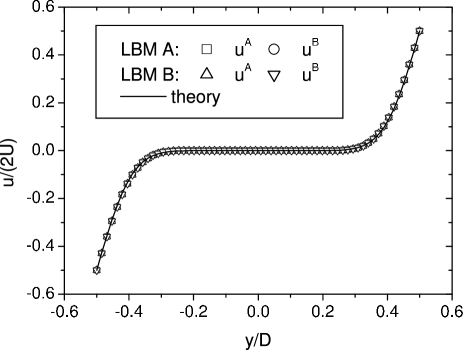
Figure 2: Horizontal velocity profiles along a vertical line for the two components at time $t=2.9$. The symbols denote simulation results from LBMs A and B. The solid line shows the analytical result. Parameters used in the simulations are $m^{A}=m^{B}=1$, $T^{A}=T^{B}=T_{\text{up}}=T_{\text{low}}=T=1$, $n^{A}=n^{B}=1$, $\gamma=0.001$. Parameters used in Eq. (138) are $\eta=0.05$, $\rho=1$.

where $u$ is the horizontal velocity, $\gamma=2U/D$ the imposed the shear rate, $j$ an integer . ( An example is referred to Fig. 2.)

Thirdly, we investigate the diffusion behavior in a one-dimensional system. To make valid the relation (77) and make less the numerical errors from the spacial FD scheme, we assume that (i) the two components have equal particle masses $1$, (ii) the initial hydrodynamic velocities of the two components are zero, (iii) the system is isothermal with temperature $T=1$, (iv) the initial density profiles of the two components are

$$\rho^{A}=\left\{\begin{array}[]{ll}1-\Delta\rho&\text{if }x\leq 0\\ 1+\Delta\rho&\text{if }x>0\end{array}\right.\text{, }\rho^{B}=\left\{\begin{array}[]{ll}1+\Delta\rho&\text{if }x\leq 0\\ 1-\Delta\rho&\text{if }x>0\end{array}\right.\text{,}$$ (139)

where $0\leq\Delta\rho\leq 1$, and (v) the viscosities of the two components are small enough. Thus, the barycentric velocity field of this system is globally zero, ${\cal D}^{A}=\tau^{AB}$, ${\cal D}^{B}=\tau^{BA}$, and the evolution of the density profiles follows

$$\rho^{A}=1+\Delta\rho\mathop{\rm erf}\left(\frac{x}{\sqrt{4{\cal D}^{A}t}}\right)\text{,}\rho^{B}=1-\Delta\rho\mathop{\rm erf}\left(\frac{x}{\sqrt{4{\cal D}^{B}t}}\right)\text{.}$$ (140)

To make the numerical tests practical, when choose parameters for simulations, the following points should be considered: (i) The accuracy of the forward Euler scheme is in the order of $\Delta t$ and that of the upwind scheme (133) is in the order of $\Delta x$; (ii) If the physical values of ${\cal D}^{A}$ and ${\cal D}^{B}$ are too small, they may be submerged by the numerical diffusivities. Numerical tests show that LBMs A and B can recover density profiles which agree well with Eq. (140). An example is shown in Fig.3. A set of density profiles for the component A are shown in (a). To help evaluate the numerical errors from the DVM, the corresponding profiles of diffusion velocity $u^{A}$ are shown in (b). The diffusion velocity $u^{A}$ has its maximum value at $x=0$. Its magnitude decreases with time. For the earliest time ($t=0.01$) shown in this figure, $\left|u^{A}\right|\approx 0.028$. The numerical errors for $f_{ki}^{A\left(0\right)}$ are in the order of $\left(u^{A}\right)^{4}$ for LBM B and in the order of $\left(u^{A}\right)^{5}$ for LBM A.

V Conclusions and remarks

Sirovich’s original two-fluid BGK kinetic theory works for symmetric systems where the two components have approximately the same total masses and local temperatures. This theory is clarified and generalized to describe both symmetric and asymmetric systems. Corresponding to different situations five kinetic models are formulated. Based on an octagonal discrete velocity model the five models are discretized. The discrete-velocity kinetic models and the continuous ones are required to recover the same Euler and/or Navier-Stokes equations. A discrete-velocity kinetic model and an appropriate finite-difference scheme compose a FDLBM. The formulated kinetic models work also for binary mixtures with disparate particle-mass components. Which model to use depends on the mean temperatures and the mean mass densities of the two components.

In the present two-fluid treatment, the relaxation times of the cross-collisions contribute to both the viscous and diffusive effects. The interfacial tension is another aspect of thermodynamic interaction between component fluids. Investigating the interfacial tension is crucial in the industrial context for controlling the size and phase stability of mechanically dispersed droplets and other transient structures formed in the course of phase separation. For immiscible fluids, one way to introduce the interfacial tension is through modifying the pressure tensorsEPL32463 by taking into account the the interparticle interactions. One possibility of incorporating the interparticle interaction is through modifying the force terms in Boltzmann equationsVictorPRE . In such a case, the force terms in the BGK kinetic models are responsible for the phase separation and interfacial tension. The acceleration ${\bf a}^{A}$ is determined by the interparticle interactions and the external field. The determination of the specific form of ${\bf a}^{A}$ depends on the system under consideration. An interesting point is that the incorporation of the force term in the Boltzmann equation makes no additional requirement on the formulation process of the FDLBM. So the specific forces can be directly considered under the same frame. A different attempt to introduce the interfacial tension is to start from the Enskog equations for dense gasesPRE6835302 .

Figure 1: Velocity and temperature equalibrations in uniform relaxation processes. The common parameters used in (a) are $n^{A}=1$,$n^{B}=2$, $m^{A}=2$, $m^{B}=1$, $\tau^{AA}=\tau^{BB}=\tau^{AB}=\tau^{BA}=1$. Additionally, $u^{A(0)}_{x}=-u^{B(0)}_{x}=0.3$, $u^{A(0)}_{y}=u^{B(0)}_{y}=0$ and $T=1$ for the isothermal case; $T^{A}=1.2$, $T^{B}=0.8$, ${\bf u}^{A(0)}={\bf u}^{B(0)}={\bf 0}$ for the thermal case. The common parameters used in (b) are $n^{A}=n^{B}=1$, $m^{A}=100$, $m^{B}=1$, $\tau^{AA}=\tau^{BB}=\tau^{AB}=\tau^{BA}=1$, $u^{A(0)}_{x}=-u^{B(0)}_{x}=0.3$, $u^{A(0)}_{y}=u^{B(0)}_{y}=0$. Additionally, $T=1$ for the isothermal case; $T^{A(0)}=10$, $T^{B(0)}=0.1$ for one and $T^{A(0)}=0.1$, $T^{B(0)}=10$ for the other thermal cases. The second superscript “(0)” denotes the initial values. Solid lines in the figure possess corresponding theoretical slopes.

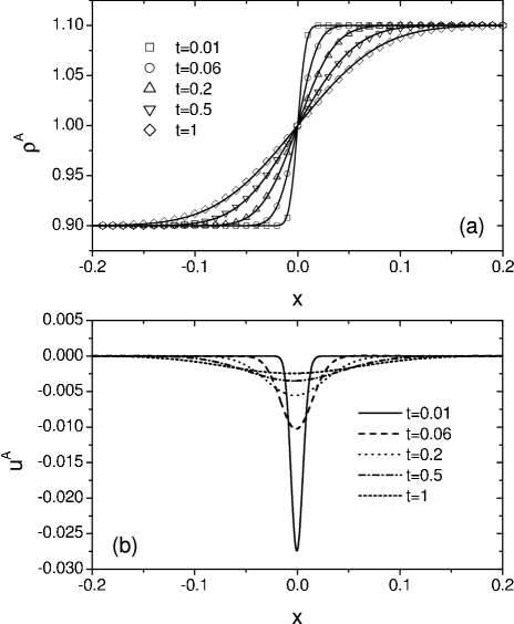
Figure 3: LBM simulation on a diffusion process. A set of density profiles of component $A$ are shown in (a) and the corresponding diffusion velocities are shown in (b). The initial density profiles of the two components follow Eq.(139) with $\Delta\rho=0.1$. All the relaxation times are taken to be $2\times 10^{-3}$. The integration steps are $\Delta x=\Delta y=10^{-4}$ and $\Delta t=10^{-5}$. The density profiles from the simulation (symbols) agree well with the theoretical ones (lines). The simulation tool for this figure is LBM A.

References

• (1) P. L. Bhatnagar, E. P. Gross, and M. Krook, Phys. Rev. 94, 511 (1954).
• (2) C. Cercignani, R. Illner and M. Pulvirenti, The mathematical theory of dilute gases, Applied Mathematical Sciences, Vol. 106, edited by F. John, J.E.Marsden, and L. Sirovich (Springer-Verlag , 1994).
• (3) F. Higuera, S. Succi, and R. Benzi, Europhys. Lett. 9, 345 (1989); R. Benzi, S. Succi, and M. Vergassola, Phys. Rep. 222, 145 (1992); S. Succi, The Lattice Boltzmann Equation (Oxford University Press, New York, 2001); H. Chen, S. Kandasamy, S. Orszag, R. Shock, S. Succi, V. Yakhot, Science 301, 633 (2003).
• (4) Private communication with S. Succi.
• (5) L.S. Luo and S. S. Girimaji, Phys. Rev. E 66, 035301(R) (2002);ibid 67, 36302 (2003).
• (6) H. Yu, L. S. Luo, S. S. Girimaji, Int. J. Comp. Eng. Sci. 3, 73 (2002).
• (7) A. Malevanets and J. M. Yeomans, Faraday Discss., 112, 237 (1999).
• (8) Z. Guo, T. S. Zhao, Phys. Rev. E 68, 035302(R) (2003); ibid 71, 026701 (2005).
• (9) Aiguo Xu, G. Gonnella, A. Lamura, Phys. Rev. E 67, 056105 (2003); Physica A 331, 10 (2004); ibid 344, 750 (2004); cond-mat/0404205; Aiguo Xu, Commun. Theor. Phys. 39, 729 (2003).
• (10) A. K. Gunstensen, D. H. Rothman, S. Zaleski, and G. Zanetti, Phys. Rev. A 43, 4320 (1991).
• (11) E. G. Flekkoy, Phys. Rev. E 47, 4247 (1993).
• (12) D. Grunau, S. Chen, and K. Eggert, Phys. Fluids A 5, 2557 (1993).
• (13) X. Shan and G. Doolen, J. Stat. Phys. 81, 379 (1995); Phys. Rev. E 54, 3614 (1996).
• (14) E. Orlandini, W. R. Osborn, and J. M. Yeomans, Europhys. Lett. 32, 463 (1995); W. R. Osborn, E. Orlandini, M. R. Swift, J. M. Yeomans, and J. R. Banavar, Phys. Rev. Lett. 75, 4031 (1995); M. R. Swift, E. Orlandini, W. R. Osborn, and J. M. Yeomans, Phys. Rev. E 54, 5041 (1996); G. Gonnella, E. Orlandini, J. M. Yeomans, Phys. Rev. Lett. 78, 1695 (1997); A. Lamura, G. Gonnella, and J. M. Yeomans, Europhys. Lett. 45, 314 (1999).
• (15) V. M. Kendon, J. C. Desplat, P. Bladon, and M.E. Cates, Phys. Rev. Lett. 83, 576 (1999); V. M. Kendon, M. E. Cates, I. Pagonabarrage, J. C. Desplat, and P. Bladon, J. Fluid Mech. 440, 147 (2001).
• (16) P.C.Facin, P.C.Philippi, and L. O. E. dos Santos, in P.M.A.Sloot et al. (Eds.): ICCS 2003, LNCS 2657, pp. 1007-1014, 2003.
• (17) A. Cristea and V. Sofonea, Central European J. Phys.2, 382 (2004); Int. J. Mod. Phys. C 14, 1251 (2003).
• (18) V. Sofonea and R. F. Sekerka, Int. J. Mod. Phys. C (in press).
• (19) V. Sofonea, A. Lamura, G. Gonnella, and A. Cristea, Phys. Rev. E 70, 046702 (2004).
• (20) X. Shan and H. Chen, Phys. Rev. E 47, 1815 (1993); ibid, 49, 2941 (1994).
• (21) P. J. Love, P.V.Coveney, and B.M.Boghosian, Phys. Rev. E 64, 21503 (2001); P. J. Love, J. B. Maillet, and P. V. Coveney, ibid 64, 61302 (2001); J. Chin, P. V. Coveney, ibid, 66, 16303 (2002); N. Gonzalez-Segredo, M. Nekovee, P. V. Coveney, ibid, 67, 46304 (2003); N. Gonzalez-Segredo, P. V. Coveney, ibid, 69, 61501 (2004).
• (22) Aiguo Xu, Europhys. Lett. 69, 214 (2005).
• (23) Victor Sofonea, Robert F. Sekerka, Physica A 299, 494 (2001).
• (24) L. Sirovich, Phys. Fluids 5, 908 (1962); ibid. 9, 2323 (1966); E. Goldman and L. Sirovich, Phys. Fluids 10, 1928 (1967).
• (25) H. W. Liepmann and A. Roshko, Elements of Gasdynamics, (New York, John Wiley & Sons, INC. 1957).
• (26) S. Chapman and T. G. Cowling, The Mathematical Theory of Non-Uniform Gases, 3rd ed. (Cambridge University Press, Cambridge, 1970).
• (27) The general BGK kinetic model of the single-component fluid can be regarded as a special case where $m^{A}=m^{B}$, $n^{A}=n^{B}$, ${\bf u}^{A}={\bf u}^{B}$, $T^{A}=T^{B}$ and consequently the cross-collision and self-collision are the same. In the Chapman-Enskog analysis we do not assume that the cross-collision terms are the first order in the Knudsen number.
• (28) M. E. Glicksman, Diffusion in Solids: Field theory, Solid-State Principles, and Applications, (John Wiley & Sons, Inc., New York, 2000).
• (29) At the Euler level, $f^{A}=f^{A(0)}$ and $f^{B}=f^{B(0)}$; but it is not required that $f^{AB(0)}=f^{A(0)}$ or $f^{BA(0)}=f^{B(0)}$, which is responsible for the momentum and heat exchanges between the two components. In the case of single-component fluidfoot1 , the terms in momentum and heat exchanges disappear.
• (30) M. Watari, M. Tsutahara, Phys. Rev. E 67, 036306 (2003).
• (31) G. Yan, Y. Chen, and S. Hu, Phys. Rev. E 59, 454 (1999).
• (32) T. Kataoka and M. Tsutahara, Phys. Rev. E 69, 056702 (2004).
• (33) V. Sofonea and R. F. Sekerka, J. Comp. Phys. 184, 422 (2003).
• (34) A. J. Wagner, Int. J. Mod. Phys. B 17, 193(2003).
• (35) C. Denniston and M. O. Robbins, Phys. Rev. E 69, 021505 (2004).
• (36) T. Seta and R. Takahashi, J. Stat. Phys. 107, 557 (2002).
• (37) H.He, L.S.Luo, J. Stat. Phys. 88, 927 (1997).
• (38) H.P. Fang, R.Z. Wan, Z.F. Lin, Phys. Rev. E 66, 036314 (2002).
Refer to caption