Observable Dependent Quasi-Equilibrium in Slow Dynamics

Abstract

We present examples demonstrating that quasi-equilibrium fluctuation-dissipation behavior at short time differences is not a generic feature of systems with slow non-equilibrium dynamics. We analyze in detail the non-equilibrium fluctuation-dissipation ratio $X(t,t_{\mathrm{w}})$ associated with a defect-pair observable in the Glauber-Ising spin chain. It turns out that $X\neq 1$ throughout the short-time regime and in particular $X(t_{\mathrm{w}},t_{\mathrm{w}})=3/4$ for $t_{\mathrm{w}}\to\infty$. The analysis is extended to observables detecting defects at a finite distance from each other, where similar violations of quasi-equilibrium behaviour are found. We discuss our results in the context of metastable states, which suggests that a violation of short-time quasi-equilibrium behavior could occur in general glassy systems for appropriately chosen observables.

INTRODUCTION

It is a common notion that in the non-equilibrium dynamics of glassy systems, fluctuations of microscopic quantities are essentially at equilibrium at short times, before the system displays aging. The concept of inherent structures or metastable states Stillinger and Weber (1984), for instance, is closely related to this picture. There, one partitions phase space into basins of attraction, e.g., corresponding to energy minima. At short times the system is expected to remain trapped in such metastable states, leading to equilibrium-type fluctuations, but activated inter-basin transitions eventually produce a signature of the underlying slow non-equilibrium evolution.

A now standard procedure for characterizing how far a system is from equilibrium is provided by the non-equilibrium violation of the fluctuation-dissipation theorem (FDT) Cugliandolo and Kurchan (1993); Cugliandolo et al. (1997a); Crisanti and Ritort (2003). Starting from a non-equilibrium initial state prepared at time $t=0$ one considers, for $t\geq t_{\mathrm{w}}\geq 0$,

$$R(t,t_{\mathrm{w}})=X(t,t_{\mathrm{w}})\frac{\partial}{\partial t_{\mathrm{w}}}C(t,t_{\mathrm{w}}),$$ (1)

where $C(t,t_{\mathrm{w}})=\langle A(t)B(t_{\mathrm{w}})\rangle-\langle A(t)\rangle\langle B(t_{\mathrm{w}})\rangle$ is the connected two-time correlation function between some observables $A,B$ and $R(t,t_{\mathrm{w}})=T\left.\delta\langle A(t)\rangle/\delta h(t_{\mathrm{w}})\right|_{h=0}$ is the conjugate response function; the perturbation associated with the field $h$ is $\delta\mathcal{H}=-h(t)B$. Note that we have absorbed the temperature $T$ into our definition of the response function. Thus, for equilibrium dynamics, FDT implies that the fluctuation-dissipation ratio (FDR) $X(t,t_{\mathrm{w}})$ defined by (1) always equals one. Correspondingly, a parametric fluctuation-dissipation (FD) plot of the susceptibility $\chi(t,t_{\mathrm{w}})=\int_{t_{\mathrm{w}}}^{t}d\tau\,R(t,\tau)$ versus $C(t,t)-C(t,t_{\mathrm{w}})$ has slope $X=1$. In systems exhibiting slow dynamics and aging, on the other hand, the FDR $X(t,t_{\mathrm{w}})$ is often found to have a non-trivial scaling form in the limit of long times Crisanti and Ritort (2003). Over short observation intervals $\Delta t=t-t_{\mathrm{w}}$ and at large waiting times $t_{\mathrm{w}}$, however, one expects to recover equilibrium FDT with $X(t,t_{\mathrm{w}})=1$ according to, e.g., the inherent structure picture. Such “quasi-equilibrium” behavior at short times has been observed in essentially all previous studies Crisanti and Ritort (2003) involving microscopic observables.

Rigorous support is given to the quasi-equilibrium scenario in Cugliandolo et al. (1997b). There a general class of systems governed by dissipative Langevin dynamics is considered. Based on the entropy production rate in non-equilibrium dynamics, a bound is derived for the differential violation $V(t,t_{\mathrm{w}})$ of FDT,

$$V(t,t_{\mathrm{w}})=\frac{\partial C}{\partial t_{\mathrm{w}}}-R=\left[1-X(t,t_{\mathrm{w}})\right]\frac{\partial C(t,t_{\mathrm{w}})}{\partial t_{\mathrm{w}}}.$$ (2)

The bound implies that under rather general assumptions Cugliandolo et al. (1997b) and for observables only depending on a finite number of degrees of freedom one has $V(t,t_{\mathrm{w}})\to 0$ for any $\Delta t\geq 0$ fixed and $t_{\mathrm{w}}\to\infty$; we call this the ”short-time regime” from now on. Via (2) it is concluded that $X(t,t_{\mathrm{w}})\to 1$ in the short-time regime. Clearly, however, the last step in this reasoning is only justified if $\lim_{t_{\mathrm{w}}\to\infty}(\partial/\partial t_{\mathrm{w}})C(t,t_{\mathrm{w}})$ at fixed $\Delta t$ is non-vanishing. This will be the case if, for example, $C(t,t_{\mathrm{w}})$ admits a decomposition into stationary and aging parts Bouchaud et al. (1998) at large $t_{\mathrm{w}}$,

$$C(t,t_{\mathrm{w}})=C_{\mathrm{st}}(t-t_{\mathrm{w}})+C_{\mathrm{ag}}(t,t_{\mathrm{w}}).$$ (3)

On the other hand, if $C(t_{\mathrm{w}},t_{\mathrm{w}})\to 0$ for $t_{\mathrm{w}}\to\infty$ then also $\lim_{t_{\mathrm{w}}\to\infty}(\partial/\partial t_{\mathrm{w}})C(t,t_{\mathrm{w}})$ will normally vanish. For such observables, $X(t,t_{\mathrm{w}})$ can a priori take arbitrary values in the short-time regime without violating the bound on $V(t,t_{\mathrm{w}})$ derived in Cugliandolo et al. (1997b).

In (3), the stationary contribution can be defined formally as $C_{\mathrm{st}}(\Delta t)=\lim_{t_{\mathrm{w}}\to\infty}C(\Delta t+t_{\mathrm{w}},t_{\mathrm{w}})$. If $C_{\mathrm{st}}(\Delta t)$ has a nonzero limit for $\Delta t\to\infty$, then this is conventionally included in $C_{\mathrm{ag}}$ instead. One then finds that the remainder, $C_{\mathrm{ag}}$, is an “aging” function: for large times it typically depends only on the ratio $t/t_{\mathrm{w}}$. Correlation functions of the form (3) are often found in aging systems, for instance when considering local spin-observables $A=B=\sigma_{i}$ in critical ferromagnets Godrèche and Luck (2002); here $C_{\mathrm{ag}}$ also contains an overall $t_{\mathrm{w}}$-dependent amplitude factor. Further examples would be spin observables in $p$-spin models Cugliandolo and Kurchan (1993) or density fluctuations in MCT Götze and Sjögren (1992). In either case the stationary correlations $C_{\mathrm{st}}(t-t_{\mathrm{w}})$ are intrinsically equilibrium-related [bulk fluctuations, dynamics within metastable states, ”cage rattling”] and quasi-equilibrium behaviour is enforced by the bound of Cugliandolo et al. (1997b). Beyond that, however, there are various examples in the recent literature Mayer et al. (2003); Buhot and Garrahan (2002); Buhot (2003) displaying quasi-equilibrium behaviour even though $C(t_{\mathrm{w}},t_{\mathrm{w}})\to 0$ for $t_{\mathrm{w}}\to\infty$. In the context of ferromagnets and spin-facilitated models such correlations are obtained when considering domain-wall or defect observables $A=B=n_{i}$. A generalization of (3) accounting for the decrease of equal time correlations with $t_{\mathrm{w}}$ is

$$C(t,t_{\mathrm{w}})=A(t_{\mathrm{w}})c_{\mathrm{st}}(t-t_{\mathrm{w}})+C_{\mathrm{ag}}(t,t_{\mathrm{w}}).$$ (4)

In the short-time contribution $C_{\mathrm{st}}(t,t_{\mathrm{w}})=A(t_{\mathrm{w}})c_{\mathrm{st}}(t-t_{\mathrm{w}})$ , $c_{\mathrm{st}}$ is now defined as $c_{\mathrm{st}}(\Delta t)=\lim_{t_{\mathrm{w}}\to\infty}C(\Delta t+t_{\mathrm{w}},t_{\mathrm{w}})/A(t_{\mathrm{w}})$. It is useful to fix $c_{\mathrm{st}}(0)=1$, so that $A(t_{\mathrm{w}})$ must behave asymptotically as the equal-time correlation $C(t_{\mathrm{w}},t_{\mathrm{w}})$. Results for defect observables in one and two-dimensional Ising models Mayer et al. (2003) are compatible with this scaling. For the one-dimensional FA and East models a similar picture emerges and it has been conjectured that aging contributions are in fact absent Buhot and Garrahan (2002); Buhot (2003). We discuss the scaling (4) and its implications in more detail below. It is clear, however, that if $C(t,t_{\mathrm{w}})\sim A(t_{\mathrm{w}})c_{\mathrm{st}}(t-t_{\mathrm{w}})$ and also $R(t,t_{\mathrm{w}})\sim A(t_{\mathrm{w}})r_{\mathrm{st}}(t-t_{\mathrm{w}})$ in the short-time regime [where $\sim$ denotes asymptotic similarity for $t_{\mathrm{w}}\to\infty$] then quasi-equilibrium behaviour requires  that $r_{\mathrm{st}}(t-t_{\mathrm{w}})=(\partial/\partial t_{\mathrm{w}})c_{\mathrm{st}}(t-t_{\mathrm{w}})$. The results of Mayer et al. (2003); Buhot and Garrahan (2002); Buhot (2003) indeed support this link.

Recently, the authors of Sastre et al. (2003) have exploited the notion of quasi-equilibrium to define a nominal system temperature $T_{\mathrm{dyn}}$ even for models where a thermodynamic bath temperature $T$ does not a priori exist, e.g., because the dynamics does not obey detailed balance. $T_{\mathrm{dyn}}$ is determined from the short-time dynamics of correlations and responses, and the authors of Sastre et al. (2003) argue that for systems coupled to a heat bath this definition should generically reduce to $T_{\mathrm{dyn}}=T$. They in fact attempt a proof of this statement , for spin models in the universality class of the two-dimensional Ising model.

The dependence of $X(t,t_{\mathrm{w}})$ on the pair of observables $A,B$ used to probe non-equilibrium FDT, Eq. (1), in finite-dimensional systems is still an actively debated issue Berthier and Barrat (2002a, b); Fielding and Sollich (2002); Sollich et al. (2002); Mayer et al. (2003); Crisanti and Ritort (2003). This is of particular relevance as regards the possibility of characterizing the slow dynamics in glassy systems by a time-scale dependent effective temperature $T_{\mathrm{eff}}=T/X(t,t_{\mathrm{w}})$ Cugliandolo et al. (1997a). Beyond mean-field models one does not expect $X(t,t_{\mathrm{w}})$, or more precisely its long time scaling, to be completely robust against the choice of $A,B$. Instead, it has been suggested that there may only be a limited class of “neutral” observables which allow a measurement of effective temperatures Sollich et al. (2002); Crisanti and Ritort (2003). It then seems plausible that also the notion of quasi-equilibrium in the short-time regime may not hold for all observables. This prompts us to revisit the observable dependence of short-time fluctuation-dissipation relations.

To be able to carry out explicit calculations, we study a simple coarsening system, the one-dimensional ferromagnetic Ising spin chain with Glauber dynamics. Coarsening systems are, of course, different from glasses but they do exhibit aging behavior, easily interpretable because of its link to a growing length scale. This makes them useful “laboratory” systems for testing general ideas and concepts developed for systems with slow dynamics. The dynamical length scale in a coarsening system – which in our case is just the typical domain size – allows one to distinguish equilibrated modes from slowly evolving non-equilibrium modes. For spatially localized observables one thus naively expects quasi-equilibrium dynamics at short times, as soon as the domain size has become much larger than the length scale probed by the observable. But, as we will see in the following, this is not true in general: there are many local observables that do not obey the equilibrium FDT even in the short-time regime. Such nontrivial violations of quasi-equilibrium behaviour have to be distinguished from what is found for global observables such as, for example, the magnetization Mayer et al. (2003): these depend on an extensive number of degrees of freedom, hence the bound of Cugliandolo et al. (1997b) does not apply and one would not expect quasi-equilibrium behaviour at short times. In coarsening systems this is also physically transparent: global observables measure the dynamics on lengthscales larger than the typical domain size, where equilibration has not yet taken place.

We analyze the non-equilibrium FDT in the Glauber-Ising chain for observables that probe correlations between domain walls (defects) at distances $d\geq 1$. In Section I we define our two-time correlation and response functions; their exact derivation for the case $d=1$ is sketched in the Appendix. We then recall some useful facts about the domain size distribution, both in and out-of equilibrium. In Sections II and III we study adjacent defects, i.e. $d=1$. Some features of the equilibrium dynamics, where FDT is obviously satisfied, are discussed in Section II. The low temperature coarsening dynamics are then analyzed in Section III and compared to the baseline provided by the equilibrium results. In particular, we focus on the short-time regime in Sections III.1–III.3. The aging behaviour is discussed in Section III.4 while Section III.5 deals with the crossover to equilibrium. Based on the understanding developed for $d=1$, nonequilibrium FD relations for defects at distances $d>1$ are then studied in Section IV. We conclude in the final section with a summary and discussion.

I Defect pair observables

In order to obtain nontrivial fluctuation-dissipation behaviour in the short-time regime we have to consider non-standard observables; in the Glauber-Ising chain local spin as well as defect observables satisfy quasi-equilibrium Godrèche and Luck (2000); Lippiello and Zannetti (2000); Mayer et al. (2003). However, as already mentioned in Mayer et al. (2003), multi-defect observables are potentially interesting candidates for new results. The simplest choice in this class are the defect-pair observables $A_{d}=n_{i}n_{i+d}$ with $d\geq 1$. We introduce the connected two-time autocorrelation functions associated with $A_{d}$ as

$$C_{d}(t,t_{\mathrm{w}}) = \langle n_{i}(t)n_{i+d}(t)n_{i}(t_{\mathrm{w}})n_{i+d}(t_{\mathrm{w}})\rangle$$ (5)

$$-\langle n_{i}(t)n_{i+d}(t)\rangle\langle n_{i}(t_{\mathrm{w}})n_{i+d}(t_{\mathrm{w}})\rangle.$$

The local two-time defect-pair response functions are

$$R_{d}(t,t_{\mathrm{w}})=T\left.\frac{\delta\langle n_{i}(t)n_{i+d}(t)\rangle}{\delta h(t_{\mathrm{w}})}\right|_{h=0},$$ (6)

where the perturbation $\delta\mathcal{H}=-h(t)n_{i}n_{i+d}$ is applied. Throughout the paper we use the short-hands $C\equiv C_{1}$ and $R\equiv R_{1}$ for the case $d=1$. Our subsequent analysis of $C$ and $R$ is based on exact expressions, see Appendix. Since $A_{d}$ is nonzero only if we simultaneously have defects at sites $i$ and $i+d$, its behavior will reflect the domain size distribution in the system, and an understanding of the latter will be useful.

I.1 Domain Size Distribution

To summarize briefly, the Glauber-Ising chain Glauber (1963) is defined on a one-dimensional lattice of Ising spins $\sigma_{i}=\pm 1$ with Hamiltonian $\mathcal{H}=-J\sum_{i}\sigma_{i}\sigma_{i+1}$, where each spin $\sigma_{i}$ flips with rate $w_{i}(\boldsymbol{\sigma})=\frac{1}{2}[1-\frac{1}{2}\gamma\sigma_{i}(\sigma_{i-1}+\sigma_{i+1})]$; here $\gamma=\tanh(2J/T)$. In terms of the domain-wall indicators or defect variables $n_{i}=\frac{1}{2}\left(1-\sigma_{i}\sigma_{i+1}\right)\in\{0,1\}$ the density of domains $D_{k}$ of given size $k$ is expressed, using translational invariance, as

$$D_{k}=\langle n_{0}(1-n_{1})\cdots(1-n_{k-1})n_{k}\rangle.$$ (7)

As usual $\langle\,\cdot\,\rangle$ refers to the ensemble average in the case of equilibrium and otherwise to an average over initial configurations and stochasticity in the dynamics.

In equilibrium the derivation of $D_{k}$ for the Glauber-Ising chain is straightforward: from $\langle\prod_{i}n_{i}\rangle=\prod_{i}\langle n_{i}\rangle$ and translational invariance we have

$$D_{k,\mathrm{eq}}=\langle n_{0}\rangle^{2}\left[1-\langle n_{0}\rangle\right]^{k-1}.$$ (8)

The distribution of domain sizes $k$ is thus exponential in equilibrium, with the most frequent domains those of size one. The mean domain size, on the other hand, is given by the inverse of the concentration of defects $\langle n_{0}\rangle$. One easily shows that

$$c_{\mathrm{eq}}(\tau_{\mathrm{eq}})=\langle n_{0}\rangle=\frac{1}{\sqrt{2\tau_{\mathrm{eq}}}}\,\frac{\sqrt{1+\gamma}-\sqrt{1-\gamma}}{\sqrt{2}\,\gamma}.$$ (9)

For equilibrium quantities we generally use the equilibration time $\tau_{\mathrm{eq}}=1/(1-\gamma)\sim\frac{1}{2}\exp(4J/T)$ to parametrize temperature. At low $T$ the defect concentration scales as $c_{\mathrm{eq}}\sim(2\tau_{\mathrm{eq}})^{-1/2}$. Hence the mean domain size is $O\left(\sqrt{\tau_{\mathrm{eq}}}\right)$. From (8), (9) the density of small domains with size $k=O(1)$ is then flat, $D_{k,\mathrm{eq}}\sim 1/(2\tau_{\mathrm{eq}})$.

We note briefly that our $D_{k}$ are densities of domains of given size, rather than a normalized domain size distribution. The normalization factor is simply the defect concentration since, from (8), $\sum_{k=1}^{\infty}D_{k}=\langle n_{0}\rangle$. Abbreviating $c=\langle n_{0}\rangle$, we can thus write $D_{k}=cP_{k}$ with $\sum_{k=1}^{\infty}P_{k}=1$. For small $c$, the normalized distribution $P_{k}$ often assumes a scaling form, with $k$ scaled by the mean domain size $1/c$: $P_{k}=cP(\kappa)$ with $\kappa=kc$, and correspondingly $D_{k}=c^{2}P(\kappa)$. From (8), the equilibrium scaling function is exponential, $P(\kappa)=\exp(-\kappa)$.

For the out-of-equilibrium case a derivation of $D_{k}$ is rather less trivial; a corresponding calculation for the $1d$ Potts model is given in Derrida and Zeitak (1996). For the Ising case and a quench at time $t=0$ from a random, uncorrelated initial state to zero temperature, the results are as follows: the mean domain size grows as $c^{-1}=O\left(\sqrt{t}\right)$ with typical domains having a concentration $O(c^{2})=O\left(t^{-1}\right)$. For large domain sizes, $k\gg\sqrt{t}$, $D_{k}(t)$ has an exponential tail $O\left((1/t)\exp(-\alpha\,k/\sqrt{t})\right)$; an expression for the constant $\alpha$ is given in Derrida and Zeitak (1996). The density of small domains $k\ll\sqrt{t}$, on the other hand, is linearly related to the domain size, with $D_{k}(t)=O\left(k/t^{3/2}\right)$. Correspondingly, the scaling form $P(\kappa)$ of the normalized domain size distribution decays exponentially for large $\kappa$, but is linear in $\kappa$ for $\kappa\ll 1$.

The precise scaling of the density of small domains $k=O(1)$ in nonequilibrium coarsening is easily derived. Instead of directly working out the $D_{k}$, which is cumbersome, consider for a moment the quantity

$$\widetilde{D}_{k}=\langle n_{0}(1-2n_{1})\cdots(1-2n_{k-1})n_{k}\rangle.$$ (10)

In contrast to the $D_{k}$, any $\widetilde{D}_{k}$ can be conveniently expanded in terms of two-spin correlations. We have, in fact, $\widetilde{D}_{k}=\frac{1}{4}\langle\sigma_{1}\sigma_{k}-\sigma_{0}\sigma_{k}-\sigma_{1}\sigma_{k+1}+\sigma_{0}\sigma_{k+1}\rangle$. For zero-temperature coarsening one shows Mayer and Sollich (2004)

$$\widetilde{D}_{k}(t)=\frac{k}{2}\,e^{-2t}\frac{I_{k}(2t)}{2t},$$ (11)

where the $I_{n}(x)$ are modified Bessel functions Gradshteyn and Ryzhik (2000). Now compare the definitions of $D_{k}$ and $\widetilde{D}_{k}$ in the limit of large times. For both quantities we have that only states with $n_{0}=n_{k}=1$ contribute. To leading order these states do not contain any further defects $n_{i}$ in the range $i=1,\ldots,k-1$, hence $D_{k}\sim\widetilde{D}_{k}\sim k/\left(8\sqrt{\pi}t^{3/2}\right)$ for $t\to\infty$. States that do contain further defects in this range, on the other hand, cause $D_{k}$ to differ from $\widetilde{D}_{k}$. In an independent interval approximation, which gives the correct scaling but incorrect prefactors Alemany and Benavraham (1995); Derrida and Zeitak (1996), the chances to have an additional defect at site $i$ are $D_{i}D_{k-i}=O\left(t^{-3}\right)$. Contributions from states containing more than one defect in this range are even smaller, giving overall $D_{k}=\widetilde{D}_{k}+O\left(t^{-3}\right)$. By the same reasoning we also have $\langle n_{i}n_{i+k}\rangle=\widetilde{D}_{k}+O\left(t^{-3}\right)$. These scalings apply for any fixed $k\geq 2$ and in the limit of large $t$. For $k=1$, finally, we have $\langle n_{i}n_{i+1}\rangle=D_{1}=\widetilde{D}_{1}$ as the definitions coincide in this case.

Note that when comparing only the scale of typical domains in and out of equilibrium, an out-of-equilibrium system of age $t$ is comparable to an equilibrium system with equilibration time $\tau_{\mathrm{eq}}\approx t$. Indeed, typical domains have size $O\left(\sqrt{\tau_{\mathrm{eq}}}\right)$ and density $O\left(\tau_{\mathrm{eq}}^{-1}\right)$ in equilibrium, while out of equilibrium the same quantities scale like $O\left(\sqrt{t}\right)$ and $O\left(t^{-1}\right)$, respectively. However, this correspondence does not extend to the details of the shape of the domain size distribution. In particular, it breaks down for small domains $k=O(1)$. In equilibrium such domains have a concentration $O\left(\tau_{\mathrm{eq}}^{-1}\right)$ while in the corresponding coarsening situation their concentration $O\left(k/t^{3/2}\right)$ is much smaller.

It is instructive to note that Glauber dynamics for the spin system $\{\sigma_{i}\}$ corresponds to a diffusion limited reaction process Santos (1997) for the defects $\{n_{i}\}$; the diffusion rate is $\frac{1}{2}$. At low $T$ adjacent defects annihilate with rate close to one while pair creation, i.e., flipping a spin within a domain, occurs with rate $1/(2\tau_{\mathrm{eq}})$. The latter process is important in equilibrium – continuously producing new domains of size one – but is unimportant at low temperatures while the system is coarsening, and indeed strictly absent at zero temperature. This leads to the different scalings of the density of small domains in and out of equilibrium.

II Equilibrium

In order to familiarize ourselves with the dynamics of defect pairs we now study the equilibrium behavior of the two-time correlation $C(t,t_{\mathrm{w}})$. An exact expression is obtained from the result for a quench to finite temperature given in the Appendix by taking the limit $t_{\mathrm{w}}\to\infty$ at fixed $\Delta t=t-t_{\mathrm{w}}$. We use the notation $C_{\mathrm{eq}}(\Delta t,\tau_{\mathrm{eq}})=\lim_{t_{\mathrm{w}}\to\infty}C(\Delta t+t_{\mathrm{w}},t_{\mathrm{w}})$ for the equilibrium correlation; from (55) one has

$$C_{\mathrm{eq}}(\Delta t,\tau_{\mathrm{eq}}) = \frac{1}{2\gamma\tau_{\mathrm{eq}}}H_{1,\mathrm{eq}}(\Delta t)\bigg{\{}e^{-\Delta t}[I_{0}-I_{1}](\gamma\Delta t)$$ (12)

$$-\frac{1}{2\gamma\tau_{\mathrm{eq}}}H_{1,\mathrm{eq}}(\Delta t)\bigg{\}}.$$

Here we have introduced the short hand $[\,\cdot\,](x)$ to indicate that all functions enclosed in the square brackets have argument $x$. The function $H$ is introduced in (53) and discussed in the Appendix. Because FDT is satisfied in equilibrium the conjugate response to (12) is $R_{\mathrm{eq}}(\Delta t,\tau_{\mathrm{eq}})=-\partial_{\Delta t}C_{\mathrm{eq}}(\Delta t,\tau_{\mathrm{eq}})$. Consequently the equilibrium susceptibility is given by

$$\chi_{\mathrm{eq}}(\Delta t,\tau_{\mathrm{eq}})=C_{\mathrm{eq}}(0,\tau_{\mathrm{eq}})-C_{\mathrm{eq}}(\Delta t,\tau_{\mathrm{eq}}),$$ (13)

and we subsequently focus on the discussion of $C_{\mathrm{eq}}$.

II.1 Small $\Delta t$ Regime

Let us first consider the dynamics of $C_{\mathrm{eq}}(\Delta t,\tau_{\mathrm{eq}})$ for finite $\Delta t\geq 0$ and in the limit of low temperatures $\tau_{\mathrm{eq}}\gg 1$. Via the definition (5) of $C\equiv C_{1}$ the equal-time value $C_{\mathrm{eq}}(0,\tau_{\mathrm{eq}})=\langle n_{i}n_{i+1}\rangle-\langle n_{i}n_{i+1}\rangle^{2}$ is directly linked to the density of domains of size one, $D_{1,\mathrm{eq}}(\tau_{\mathrm{eq}})=\langle n_{i}n_{i+1}\rangle$. From (8), (9) and setting $\Delta t=0$ in (12)

$$D_{1,\mathrm{eq}}(\tau_{\mathrm{eq}})=\frac{1}{2\tau_{\mathrm{eq}}}\frac{1-\sqrt{1-\gamma^{2}}}{\gamma^{2}}=\frac{1}{2\gamma\tau_{\mathrm{eq}}}H_{1,\mathrm{eq}}(0).$$ (14)

At low temperatures $D_{1,\mathrm{eq}}(\tau_{\mathrm{eq}})$ and thus $C_{\mathrm{eq}}(0,\tau_{\mathrm{eq}})$ scales as $D_{1,\mathrm{eq}}(\tau_{\mathrm{eq}})\sim 1/(2\tau_{\mathrm{eq}})$. Now, for finite $\Delta t>0$ and in the limit of low temperatures $\tau_{\mathrm{eq}}\gg 1$ an expansion of (12) gives, to leading order,

$$C_{\mathrm{eq}}(\Delta t,\tau_{\mathrm{eq}})=p_{1}(\Delta t)D_{1,\mathrm{eq}}(\tau_{\mathrm{eq}})+O\left(\tau_{\mathrm{eq}}^{-2}\right),$$ (15)

where

$$p_{1}(\Delta t)=e^{-2\Delta t}[I_{0}^{2}-I_{1}^{2}](\Delta t).$$ (16)

From (15) and our knowledge of the equilibrium domain size distribution we may assign a direct physical meaning to $p_{1}(\Delta t)$: in the limit of low temperatures and at finite $\Delta t$ the connected and disconnected correlations coincide to leading order, i.e., $C_{\mathrm{eq}}(\Delta t,\tau_{\mathrm{eq}})\sim\langle n_{i}(\Delta t)n_{i+1}(\Delta t)n_{i}(0)n_{i+1}(0)\rangle$. So only situations where sites $i$ and $i+1$ are occupied by defects at both times contribute to $C_{\mathrm{eq}}$. But since the size of typical domains scales as $O\left(\sqrt{\tau_{\mathrm{eq}}}\right)$, the probability for neighboring domains to be of size $O(1)$ vanishes at low temperatures. Therefore, and since $\Delta t=O(1)$, the defect pair at sites $i,i+1$ at the later time $\Delta t$ must in fact be the one that also occupied these sites at the reference time. Hence we may interpret $p_{1}(\Delta t)$ as the “random walk return probability of an adjacent defect pair”.

This scenario is easily verified by direct calculation. Consider a one-dimensional lattice containing exactly two defects at sites $k$ and $l$ with $k<l$ at time $t=0$. Denote by $p_{t}(i,j)$ the probability to find these defects at sites $i<j$ at time $t$. Since the $T=0$ dynamics of defects in the Glauber-Ising chain is diffusion-limited pair annihilation Santos (1997) with diffusion rate $\frac{1}{2}$ and annihilation rate one the $p_{t}(i,j)$ satisfy Derrida and Zeitak (1996)

$$\frac{\partial}{\partial t}p_{t}(i,j) = -2p_{t}(i,j)+\frac{1}{2}\left[p_{t}(i-1,j)+p_{t}(i+1,j)\right.$$ (17)

$$\left.+p_{t}(i,j-1)+p_{t}(i,j+1)\right].$$

This system of equations must be solved over $i<j$ subject to the boundary conditions $p_{t}(i,i)=0$. Using images Derrida and Zeitak (1996); Mayer and Sollich (2004) it is straightforward to show that the solution is

$$p_{t}(i,j)=\sum_{k<l}G_{t}(i,j;k,l)p_{0}(k,l),$$ (18)

where

$$G_{t}(i,j;k,l)=e^{-2t}\left[I_{i-k}I_{j-l}-I_{i-l}I_{j-k}\right](t).$$ (19)

It is clear from this result that the Green’s function $G_{t}(i,j;k,l)$ is in fact the conditional probability of finding the defect-pair at sites $i<j$ at time $t$ given that it was initially located at sites $k<l$. Consequently $p_{1}(t)=G_{t}(i,i+1;i,i+1)$ as claimed above. The two-time defect-pair correlation $C_{\mathrm{eq}}(\Delta t,\tau_{\mathrm{eq}})$, Eq. (15), is thus to leading order given by the probability $D_{1,\mathrm{eq}}(\tau_{\mathrm{eq}})$ of having a defect pair at sites $i,i+1$ times the conditional probability $p_{1}(\Delta t)$ for this pair also to occupy the same sites a time $\Delta t$ later. For $\Delta t\gg 1$ an expansion of (16) gives $p_{1}(\Delta t)\sim 1/(2\pi\Delta t^{2})$: the return probability for the defect pair drops quite rapidly as defects are likely to have disappeared via annihilation in the time interval $[0,\Delta t]$ if $\Delta t\gg 1$.

II.2 Large Times

When $\Delta t$ becomes comparable to $\tau_{\mathrm{eq}}$ the simple picture discussed above breaks down; annihilation events with remote defects and pair creation are then relevant. But from equation (12) results for this regime, which are formally obtained by taking $\Delta t,\tau_{\mathrm{eq}}\to\infty$ with their ratio fixed, are easily derived. In this limit we replace the modified Bessel functions appearing in (12) with their asymptotic expansions Gradshteyn and Ryzhik (2000). This produces the leading order scalings

$$C_{\mathrm{eq}}(\Delta t,\tau_{\mathrm{eq}}) \sim \frac{1}{4\pi\Delta t^{2}\tau_{\mathrm{eq}}}\qquad\qquad[\Delta t\ll\tau_{\mathrm{eq}}],$$ (20)

$$C_{\mathrm{eq}}(\Delta t,\tau_{\mathrm{eq}}) \sim \frac{3\tau_{\mathrm{eq}}}{16\pi\Delta t^{4}}e^{-2\Delta t/\tau_{\mathrm{eq}}}\hskip 7.92218pt[\Delta t\gg\tau_{\mathrm{eq}}].$$ (21)

The expansion (20) matches the large $\Delta t$ limit of (15). So up to the time scale $\Delta t=O(\tau_{\mathrm{eq}})$ the decay of the connected two-time defect pair correlation is controlled by the defect pair return probability. For times $\Delta t$ beyond $O(\tau_{\mathrm{eq}})$, defect configurations are reshuffled via pair creation and the connected correlation vanishes exponentially as one might expect. For later reference we note that according to (15), (20), (21) we have $C_{\mathrm{eq}}(\Delta t,\tau_{\mathrm{eq}})>0$ at all times.

There is, however, a subtle effect in the underlying physics. This becomes obvious when considering disconnected correlation functions. The disconnected defect pair correlation in equilibrium is $C_{\mathrm{eq}}^{\mathrm{DC}}(\Delta t,\tau_{\mathrm{eq}})=\langle n_{i}(\Delta t)n_{i+1}(\Delta t)n_{j}(0)n_{j+1}(0)\rangle$, and is linked to the connected one via $C_{\mathrm{eq}}^{\mathrm{DC}}(\Delta t,\tau_{\mathrm{eq}})=C_{\mathrm{eq}}(\Delta t,\tau_{\mathrm{eq}})+D_{1,\mathrm{eq}}^{2}(\tau_{\mathrm{eq}})$. Now according to (14) we have $D_{1,\mathrm{eq}}^{2}(\tau_{\mathrm{eq}})=O\left(\tau_{\mathrm{eq}}^{-2}\right)$ while from (20), $C_{\mathrm{eq}}(\Delta t,\tau_{\mathrm{eq}})=O\left(\Delta t^{-2}\tau_{\mathrm{eq}}^{-1}\right)$ for $\Delta t\ll\tau_{\mathrm{eq}}$. Therefore, if $\Delta t\gg\sqrt{\tau_{\mathrm{eq}}}$, $C_{\mathrm{eq}}(\Delta t,\tau_{\mathrm{eq}})$ is negligible compared to $D_{1,\mathrm{eq}}^{2}(\tau_{\mathrm{eq}})$ and so the disconnected correlation $C_{\mathrm{eq}}^{\mathrm{DC}}(\Delta t,\tau_{\mathrm{eq}})$ becomes $\Delta t$-independent. In other words, because of the rapid decay of the defect pair return probability $p_{1}(\Delta t)$ we are more likely to find an independent defect pair at sites $i$, $i+1$, rather than the original one, already on a time scale $\Delta t=O\left(\sqrt{\tau_{\mathrm{eq}}}\right)$. This is in marked contrast to spin or (single) defect observables Mayer and Sollich (2004), where this crossover happens on the time scale $\Delta t=O\left(\tau_{\mathrm{eq}}\right)$.

Let us finally consider the equilibrium defect pair susceptibility $\chi_{\mathrm{eq}}(\Delta t,\tau_{\mathrm{eq}})$. According to (13) it is strictly increasing, implying that $R_{\mathrm{eq}}(\Delta t,\tau_{\mathrm{eq}})>0$ at all times, and grows from its initial value of zero at $\Delta t=0$ to the asymptotic value $C_{\mathrm{eq}}(0,\tau_{\mathrm{eq}})$ on an $O(1)$ time scale. Explicitly we have from (15) the approximation $\chi_{\mathrm{eq}}(\Delta t,\tau_{\mathrm{eq}})\approx D_{1,\mathrm{eq}}(\tau_{\mathrm{eq}})[1-p_{1}(\Delta t)]$ which holds uniformly in $\Delta t$ at low temperatures.

III Non-Equilibrium

In this section we analyze defect pair correlation and response functions for zero temperature coarsening dynamics following a quench from a random, uncorrelated initial state. For the most part we will focus on the short-time behavior of these functions. Following our discussion in the introduction we decompose the two-time functions into short-time and aging contributions,

$$C(t,t_{\mathrm{w}}) = C_{\mathrm{st}}(t,t_{\mathrm{w}})+C_{\mathrm{ag}}(t,t_{\mathrm{w}}),$$ (22)

$$R(t,t_{\mathrm{w}}) = R_{\mathrm{st}}(t,t_{\mathrm{w}})+R_{\mathrm{ag}}(t,t_{\mathrm{w}}).$$ (23)

The two-time correlation and response functions are obtained from (55) and the construction of the response given in the Appendix. For mathematical simplicity we take the limit $T\to 0$ but stress that the results are also valid for nonzero temperatures $T>0$ while the system is still far from equilibrium; as discussed in Sec. III.5, this requires $t_{\mathrm{w}},t\ll{\tau_{\mathrm{eq}}}^{2/3}$. The response functions are always derived by taking the perturbing field $h$ to zero before taking $T\to 0$. This has to be done to ensure linearity of the response: as discussed in more detail below, the size of the linear regime in the field strength $h$ scales as $T$ for low $T$. We find

$$C_{\mathrm{st}}(t,t_{\mathrm{w}}) = \frac{1}{2}e^{-2t}[I_{0}^{2}-I_{1}^{2}](t-t_{\mathrm{w}})\frac{I_{1}(2t_{\mathrm{w}})}{2t_{\mathrm{w}}},$$ (24)

$$R_{\mathrm{st}}(t,t_{\mathrm{w}}) = \frac{1}{4}e^{-2t}[(I_{0}^{2}-I_{1}^{2})-I_{1}(I_{0}-I_{2})](t-t_{\mathrm{w}})$$ (25)

$$\times\frac{[I_{1}+2I_{2}](2t_{\mathrm{w}})}{2t_{\mathrm{w}}},$$

$$C_{\mathrm{ag}}(t,t_{\mathrm{w}}) = -\frac{1}{4}e^{-2(t+t_{\mathrm{w}})}\frac{I_{1}^{2}(t+t_{\mathrm{w}})}{(t+t_{\mathrm{w}})^{2}}$$ (26)

$$+\frac{1}{2}e^{-2(t+t_{\mathrm{w}})}[I_{0}-I_{1}](t-t_{\mathrm{w}})\left\{\frac{I_{1}(t+t_{\mathrm{w}})}{t+t_{\mathrm{w}}}[I_{0}+I_{1}](2t_{\mathrm{w}})-[I_{0}+I_{1}](t+t_{\mathrm{w}})\frac{I_{1}(2t_{\mathrm{w}})}{2t_{\mathrm{w}}}\right\},$$

$$R_{\mathrm{ag}}(t,t_{\mathrm{w}}) = \frac{1}{8}e^{-2(t+t_{\mathrm{w}})}[I_{0}-2I_{1}+I_{2}](t-t_{\mathrm{w}})\left\{\frac{[I_{1}+2I_{2}](t+t_{\mathrm{w}})}{t+t_{\mathrm{w}}}[I_{0}+I_{1}](2t_{\mathrm{w}})-[I_{0}+I_{1}](t+t_{\mathrm{w}})\frac{[I_{1}+2I_{2}](2t_{\mathrm{w}})}{2t_{\mathrm{w}}}\right\}$$ (27)

$$+\frac{1}{4}e^{-2(t+t_{\mathrm{w}})}[I_{1}-I_{2}](t-t_{\mathrm{w}})\left\{\frac{I_{1}(2t_{\mathrm{w}})}{2t_{\mathrm{w}}}\frac{I_{1}(t+t_{\mathrm{w}})}{t+t_{\mathrm{w}}}-\frac{[I_{1}-I_{2}](t+t_{\mathrm{w}})}{t+t_{\mathrm{w}}}[I_{0}+I_{1}](2t_{\mathrm{w}})\right\}.$$

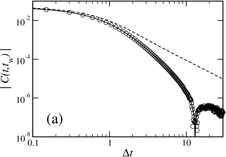
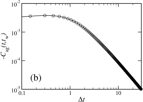
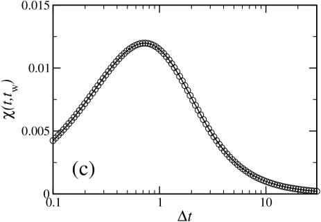
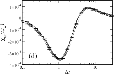
Figure 1: Comparison of our exact predictions (22- 27), shown as full curves, and simulation data [circles] at $T=0$ and $t_{\mathrm{w}}=1$. Predictions for the susceptibilities are obtained by numerical integration of (25) and (27). The data for aging contributions in panel (b) and (d) is obtained from the simulation data of $C(t,t_{\mathrm{w}})$ and $\chi(t,t_{\mathrm{w}})$ shown in (a), (c) by subtracting off the exact short-time contributions (24) [dashed line in panel (a)] and the susceptibility corresponding to (25). In panel (b) and (c) error bars for the simulation data are invisible on the scale of the plot. The same is true for (a) and $\Delta t<10$. For $\Delta t>10$, on the other hand, the standard deviation of the data is around $10^{-7}$, which is reflected in the plot. In panel (d), finally, error bars [$\pm$ standard deviation] are shown for every fifth data point but are no larger than the symbols.

As we will see in Section III.1 below, only the short-time functions (24), (25) contain terms that contribute to leading order in the short-time regime.

The results given above are exact. Before proceeding, we nevertheless compare them with simulation data to exclude the possibility of trivial algebraic errors in the derivation and confirm some of the more surprising features that are discussed below. For measuring two-time susceptibilities $\chi_{A,B}(t,t_{\mathrm{w}})$, with $A_{i},B_{i}$ generic local observables, we use the standard method Barrat (1998) of perturbing the system with $\delta\mathcal{H}=-h\sum_{i}\epsilon_{i}B_{i}$ for $t\geq t_{\mathrm{w}}$ such that $\chi_{A,B}(t,t_{\mathrm{w}})=(T/h)\sum_{i}\left[\epsilon_{i}\langle A_{i}(t)\rangle\right]_{\epsilon}$ in the limit $h\to 0$. Here the $\epsilon_{i}\in\{-1,1\}$ are independent, identically distributed random variables and $[\,\cdot\,]_{\epsilon}$ denotes an average over their distribution. Note that as our definition of the response contains a factor of $T$ this is also the case for $\chi_{A,B}(t,t_{\mathrm{w}})$. Transition rates in the presence of the perturbation are, to linear order in $h/T$,

$$w^{(h)}_{n}(\boldsymbol{\sigma}) = w_{n}(\boldsymbol{\sigma})+\frac{h}{T}w_{n}(\boldsymbol{\sigma})\left[1-w_{n}(\boldsymbol{\sigma})\right]\sum_{m}\epsilon_{n-m}$$ (28)

$$\times\left[B_{n-m}(F_{n}\boldsymbol{\sigma})-B_{n-m}(\boldsymbol{\sigma})\right].$$

Here $F_{n}\boldsymbol{\sigma}=(\ldots,-\sigma_{n},\ldots)$ denotes the spin-flip operator and $w_{n}(\boldsymbol{\sigma})$ are standard Glauber rates without perturbation. In the procedure of measuring $\chi_{A,B}(t,t_{\mathrm{w}})$ the perturbing field $h$ only appears in the combination $\bar{h}=h/T$. There is therefore a well defined zero-temperature limit at fixed $\bar{h}$; the linear susceptibility is then obtained by using a sufficiently small $\bar{h}$. We note finally that local perturbations only produce a few non-zero terms in the sum in (28). The defect pair observables $A_{i}=B_{i}=n_{i}n_{i+1}$ we are considering, for instance, only depend on $\sigma_{i},\sigma_{i+1},\sigma_{i+2}$ and thus only $m=0,1,2$ contribute to the sum in (28).

We show in Section III.4 that with increasing $t_{\mathrm{w}}$ it becomes harder to see aging contributions in the two-time correlation and response functions. In order to be able to resolve these aging contributions in a simulation we have chosen $t_{\mathrm{w}}=1$ and $\Delta t=0.1\ldots 30$. The data presented in Fig. 1 are for zero-temperature simulations in a system of $10^{6}$ spins, averaged over $10^{4}$ runs. For measuring the susceptibility we use $\bar{h}=0.2$, which is well within the linear regime. Our code uses an event driven algorithm Bortz et al. (1975) although for the small times considered here a standard Monte-Carlo method would be just as efficient. As a full discussion of $C(t,t_{\mathrm{w}})$ and $R(t,t_{\mathrm{w}})$ will be given in the subsequent sections we comment only briefly on the data in Fig. 1. According to our decomposition (22) we may think of the connected two-time defect pair correlation in Fig. 1(a) as the sum of short-time and aging contributions. From (24) short-time contributions are always positive while the aging contributions (26) are in fact negative, see Fig. 1(b). From Fig. 1(a) the correlation $C(t,t_{\mathrm{w}})$ is dominated by short-time contributions up to about $\Delta t=1$. In the range $\Delta t=1\ldots 13$ short-time and aging contributions compete, leading to a fast drop in $C(t,t_{\mathrm{w}})$. At $\Delta t\approx 13$, $C(t,t_{\mathrm{w}})$ crosses zero, giving the cusp in the plot. For $\Delta t>13$ the two-time correlation is negative, with short-time and aging contributions almost cancelling each other. The two-time defect pair susceptibility $\chi(t,t_{\mathrm{w}})$ shown in Fig. 1(c), may similarly be regarded as containing short-time and aging contributions according to (23). From Fig. 1(d) aging contributions in $\chi(t,t_{\mathrm{w}})$ are tiny such that a plot of $\chi_{\mathrm{st}}(t,t_{\mathrm{w}})$ alone would fit the data shown in Fig. 1(c) rather well. The small deviations of $\chi(t,t_{\mathrm{w}})$ from $\chi_{\mathrm{st}}(t,t_{\mathrm{w}})$, that is $\chi_{\mathrm{ag}}(t,t_{\mathrm{w}})$, however, are precisely as predicted by (27), see Fig. 1(d). Altogether, the data presented in Fig. 1 are fully consistent with, and thus confirm, our exact results (24-27). We therefore now turn to a discussion of $C(t,t_{\mathrm{w}})$, $\chi(t,t_{\mathrm{w}})$ based directly on (24-27).

III.1 Short-Time Regime

Here we analyze the dynamics of $C(t,t_{\mathrm{w}})$ and $R(t,t_{\mathrm{w}})$ in the short-time regime of $\Delta t\geq 0$ fixed and $t_{\mathrm{w}}\to\infty$. For the correlation we have from an expansion of (26) that the aging contribution scales as $C_{\mathrm{ag}}(t,t_{\mathrm{w}})=O\left(t_{\mathrm{w}}^{-3}\right)$ in this limit; already at $t_{\mathrm{w}}=10$ a plot of $C_{\mathrm{ag}}$ would lie below the vertical range of Fig.1(b). The term $C_{\mathrm{st}}(t,t_{\mathrm{w}})$, Eq. (24), on the other hand, is simply $C_{\mathrm{st}}(t,t_{\mathrm{w}})=p_{1}(t-t_{\mathrm{w}})D_{1}(t_{\mathrm{w}})$ as follows from $D_{1}=\widetilde{D}_{1}$ and (11), (16). Because $D_{1}(t_{\mathrm{w}})=O\left({t_{\mathrm{w}}}^{-3/2}\right)$, aging contributions in $C(t,t_{\mathrm{w}})$ are subdominant. In the short-time regime the connected two-time defect pair correlation is thus to leading order given by $C_{\mathrm{st}}(t,t_{\mathrm{w}})$ alone,

$$C(t,t_{\mathrm{w}})=p_{1}(t-t_{\mathrm{w}})D_{1}(t_{\mathrm{w}})+O\left(t_{\mathrm{w}}^{-3}\right).$$ (29)

This scaling property is the key that separates short-time contributions $C_{\mathrm{st}}$ from aging terms $C_{\mathrm{ag}}$ in (22), (24), (26). Furthermore $C_{\mathrm{st}}$ is of the form $C_{\mathrm{st}}(t,t_{\mathrm{w}})=A(t_{\mathrm{w}})c_{\mathrm{st}}(t-t_{\mathrm{w}})$ as proposed in (4). Comparison of (15) and (29) shows that the nonequilibrium relaxation function $c_{\mathrm{st}}(\Delta t)=p_{1}(\Delta t)$ coincides with its low-temperature equilibrium counterpart. Only the amplitude $A$ is given by the dynamical density of defect pairs $D_{1}(t_{\mathrm{w}})$ instead of its equilibrium analogue $D_{1,\mathrm{eq}}(\tau_{\mathrm{eq}})$.

The result (29) is easily explained by random walk arguments, in full analogy to Sec. II.1. Connected and disconnected correlations coincide to $O\left(D_{1}^{2}\right)=O\left(t_{\mathrm{w}}^{-3}\right)$. For the disconnected correlation to be nonzero we need states containing a defect pair at sites $i,i+1$ at time $t_{\mathrm{w}}$. These occur with probability $D_{1}(t_{\mathrm{w}})$ and to order $O\left(t_{\mathrm{w}}^{-3}\right)$ there are no further defects in any finite neighbourhood. Hence only if these defects also occupy the same sites at time $t$ is there a contribution to the disconnected correlation. This occurs with probability $p_{1}(\Delta t)=G_{\Delta t}(0,1;0,1)$ and (29) follows.

Now we turn to the behaviour of the defect pair response in the short-time regime. Expanding (27) shows that $R_{\mathrm{ag}}=O\left(t_{\mathrm{w}}^{-3}\right)$. But $R_{\mathrm{st}}=O\left({t_{\mathrm{w}}}^{-3/2}\right)$ from (25) so $R$ is dominated by $R_{\mathrm{st}}$ in the short-time regime, i.e., $R(t,t_{\mathrm{w}})=R_{\mathrm{st}}(t,t_{\mathrm{w}})+O\left(t_{\mathrm{w}}^{-3}\right)$ just as was the case for the correlations. We rearrange this result into the form

$$R(t,t_{\mathrm{w}}) = \frac{3}{4}\left[\frac{\partial}{\partial t_{\mathrm{w}}}p_{1}(t-t_{\mathrm{w}})-2e^{-2(t-t_{\mathrm{w}})}\frac{I_{1}^{2}(t-t_{\mathrm{w}})}{t-t_{\mathrm{w}}}\right]$$ (30)

$$\times D_{1}(t_{\mathrm{w}})+O\left(t_{\mathrm{w}}^{-5/2}\right),$$

where the expression in the square bracket coincides with the $\Delta t$-dependent factor in (25). The $t_{\mathrm{w}}$-dependent amplitude factor in (25) was expressed in terms of $D_{1}=\widetilde{D}_{1}$, Eq. (11), using $e^{-x}I_{2}(x)=e^{-x}I_{1}(x)+O\left(x^{-3/2}\right)$. Writing $R_{\mathrm{st}}(t,t_{\mathrm{w}})=A(t_{\mathrm{w}})r_{\mathrm{st}}(t-t_{\mathrm{w}})$ as the equivalent of (4) then shows that the nonequilibrium function $r_{\mathrm{st}}(\Delta t)$ is different from its equilibrium counter part $(-\partial/\partial\Delta t)c_{\mathrm{st}}(\Delta t)=(-\partial/\partial\Delta t)p_{1}(\Delta t)$. In fact, from $(\partial/\partial t_{\mathrm{w}})C(t,t_{\mathrm{w}})\sim[(\partial/\partial t_{\mathrm{w}})p_{1}(t-t_{\mathrm{w}})]D_{1}(t_{\mathrm{w}})$ and (30) we obtain for the FDR in the short-time regime, abbreviating $X(\Delta t)=\lim_{t_{\mathrm{w}}\to\infty}X(t,t_{\mathrm{w}})$,

$$X(\Delta t)=\frac{3}{4}\left[1-\frac{2}{(-\partial/\partial\Delta t)p_{1}(\Delta t)}e^{-2\Delta t}\frac{I_{1}^{2}(\Delta t)}{\Delta t}\right].$$ (31)

Thus the FDR is neither equal to one nor even constant in the short-time regime. In particular, for $\Delta t\to 0$ one finds

$$X(0)=\lim_{t_{\mathrm{w}}\to\infty}X(t_{\mathrm{w}},t_{\mathrm{w}})=\frac{3}{4}.$$ (32)

III.2 The Response Function

Let us now try to understand the origin for the anomalous short-time response (30). For correlations we saw that the asymptotic equality between $C$ and $C_{\mathrm{st}}$, Eq. (29), could be easily explained by random walk arguments. This is, in fact, also possible for response functions in the short regime. We use that any response function $R_{A,B}$ as defined below (1) can be written – via, e.g., the approach of Mayer and Sollich (2004) – in the form

$$R_{A,B}(t,t_{\mathrm{w}}) = \sum_{k}\sum_{\boldsymbol{\sigma},\boldsymbol{\sigma}^{\prime}}A(\boldsymbol{\sigma}^{\prime})\left[p_{\Delta t}(\boldsymbol{\sigma}^{\prime}|F_{k}\boldsymbol{\sigma})-p_{\Delta t}(\boldsymbol{\sigma}^{\prime}|\boldsymbol{\sigma})\right]$$ (33)

$$\times\Delta_{k}B(\boldsymbol{\sigma})w_{k}(\boldsymbol{\sigma})\left[1-w_{k}(\boldsymbol{\sigma})\right]p_{t_{\mathrm{w}}}(\boldsymbol{\sigma}).$$

This equation applies for general systems governed by heat-bath dynamics with Glauber rates $w_{k}$ and for generic observables $A,B$. The $p_{t_{\mathrm{w}}}(\boldsymbol{\sigma})$ denote state probabilities at time $t_{\mathrm{w}}$ while $p_{\Delta t}(\boldsymbol{\sigma}^{\prime}|\boldsymbol{\sigma})$ are conditional probabilities to go from state $\boldsymbol{\sigma}$ to $\boldsymbol{\sigma}^{\prime}$ during the time interval $\Delta t$. In (33), $\Delta_{k}B(\boldsymbol{\sigma})=B(F_{k}\boldsymbol{\sigma})-B(\boldsymbol{\sigma})$ is just a short hand expressing the change of $B$ under a spin-flip.

In the concrete case of defect pair observables $A=B=n_{i}n_{i+1}$ we have $\Delta_{k}B(\boldsymbol{\sigma})=0$ except for $k=i,i+1,i+2$. Denote the corresponding contributions to the response by $r_{1},r_{2},r_{3}$, respectively. Next work out $a_{k}=\Delta_{k}B(\boldsymbol{\sigma})w_{k}(\boldsymbol{\sigma})[1-w_{k}(\boldsymbol{\sigma})]$; it is convenient to use that Glauber rates at $T=0$ for the Ising chain may be written as $w_{k}=\frac{1}{2}(n_{k-1}+n_{k})$. It turns out that $a_{i+1}=0$ and hence $r_{2}=0$. Also, $r_{1}$ and $r_{3}$ are related by reflection symmetry so we only discuss $r_{1}$. From $a_{i}$ and (33),

$$r_{1} = \frac{1}{4}\sum_{\boldsymbol{\sigma},\boldsymbol{\sigma}^{\prime}}n_{i}n_{i+1}\left[p_{\Delta t}(\boldsymbol{\sigma}^{\prime}|F_{i}\boldsymbol{\sigma})-p_{\Delta t}(\boldsymbol{\sigma}^{\prime}|\boldsymbol{\sigma})\right]$$

$$\times[n_{i-1}(1-n_{i})n_{i+1}-(1-n_{i-1})n_{i}n_{i+1}]p_{t_{\mathrm{w}}}(\boldsymbol{\sigma}).$$

In the first line of this equation $n_{k}$ is to be read as $n_{k}(\boldsymbol{\sigma}^{\prime})$ while in the second one $n_{k}=n_{k}(\boldsymbol{\sigma})$. Now consider the term $n_{i-1}(1-n_{i})n_{i+1}$. It only contributes to $r_{1}$ for states $\boldsymbol{\sigma}$ containing defects at sites $i-1$ and $i+1$ but not at site $i$. For zero temperature coarsening and at large $t_{\mathrm{w}}$, however, we have that if there are defects on sites $i-1$ and $i+1$ then to $O(t_{\mathrm{w}}^{-3})$ there will be no further defects in any finite neighbourhood anyway. We also know that the density of states containing defects at sites $i-1,i+1$ is $\langle n_{i-1}n_{i+1}\rangle=D_{2}(t_{\mathrm{w}})+O\left(t_{\mathrm{w}}^{-3}\right)$. Next, given any such state $\boldsymbol{\sigma}$, $\sum_{\boldsymbol{\sigma}^{\prime}}n_{i}(\boldsymbol{\sigma}^{\prime})n_{i+1}(\boldsymbol{\sigma}^{\prime})p_{\Delta t}(\boldsymbol{\sigma}^{\prime}|\boldsymbol{\sigma})$ is the probability that these defects occupy sites $i,i+1$ a time $\Delta t$ later, that is $G_{\Delta t}(i,i+1;i-1,i+1)$ from (19). The state $F_{i}\boldsymbol{\sigma}$, on the other hand, has its defects on sites $i,i+1$. [To see this, note that $F_{i}$ is a spin flip operator $\sigma_{i}\to-\sigma_{i}$, so $n_{i-1}(F_{i}\boldsymbol{\sigma})=1-n_{i-1}(\boldsymbol{\sigma})$ and $n_{i}(F_{i}\boldsymbol{\sigma})=1-n_{i}(\boldsymbol{\sigma})$ using $n_{k}=\frac{1}{2}(1-\sigma_{k}\sigma_{k+1})$.] Consequently $\sum_{\boldsymbol{\sigma}^{\prime}}n_{i}(\boldsymbol{\sigma}^{\prime})n_{i+1}(\boldsymbol{\sigma}^{\prime})p_{\Delta t}(\boldsymbol{\sigma}^{\prime}|F_{i}\boldsymbol{\sigma})=G_{\Delta t}(i,i+1;i,i+1)$. Repeating this argument for the term $(1-n_{i-1})n_{i}n_{i+1}$ in $r_{1}$, where $\langle n_{i}n_{i+1}\rangle=D_{1}(t_{\mathrm{w}})+O\left(t_{\mathrm{w}}^{-3}\right)$, and working out $r_{3}$ in the same fashion then produces

$$R(t,t_{\mathrm{w}}) = \frac{1}{2}\left[G_{\Delta t}(0,1;0,1)-G_{\Delta t}(0,1;0,2)\right]$$ (34)

$$\times\left[D_{1}(t_{\mathrm{w}})+D_{2}(t_{\mathrm{w}})\right]+O\left(t_{\mathrm{w}}^{-3}\right).$$

In this result invariance of $G$ under index translation and $G_{\Delta t}(0,1;-1,1)=G_{\Delta t}(0,1;0,2)$ was used. From $D_{1}(t_{\mathrm{w}})=\widetilde{D}_{1}(t_{\mathrm{w}})$, $D_{2}(t_{\mathrm{w}})=\widetilde{D}_{2}(t_{\mathrm{w}})+O\left(t_{\mathrm{w}}^{-3}\right)$ and (11), (19) one shows that (34) precisely reproduces the short-time response $R_{\mathrm{st}}$, Eq. (25). The subdominant $O\left(t_{\mathrm{w}}^{-3}\right)$ corrections in (34) are aging contributions arising from multi-defect processes.

The structure of (34) clearly reflects the mechanisms causing a short-time response. During the time interval $[t_{\mathrm{w}},t_{\mathrm{w}}+\delta t]$ where the perturbation $\delta\mathcal{H}=-hn_{i}n_{i+1}$ is applied there is an increased likelihood for a defect pair located at sites $i,i+1$ to stay there. The effect on $\langle n_{i}(t)n_{i+1}(t)\rangle$ is accounted for by $G_{\Delta t}(0,1;0,1)D_{1}(t_{\mathrm{w}})$ in (34). Conversely, the chances for the defect on site $i+1$ to move to $i+2$ during the interval $[t_{\mathrm{w}},t_{\mathrm{w}}+\delta t]$ are decreased. The corresponding change in $\langle n_{i}(t)n_{i+1}(t)\rangle$ is proportional to $-G_{\Delta t}(0,1;0,2)D_{1}(t_{\mathrm{w}})$. By the same reasoning and starting from configurations containing defects on sites $i,i+2$ or $i-1,i+1$ one explains the remaining terms in (34). Overall, defects are on average closer to each other and more likely to occupy sites $i,i+1$ at time $t_{\mathrm{w}}+\delta t$ due to the perturbation. However, this increases the chances for subsequent annihilation of the defect pair so that we should expect $\langle n_{i}(t)n_{i+1}(t)\rangle$ to become lower than without the perturbation eventually. Indeed, from (34) and $D_{2}(t_{\mathrm{w}})\sim 2D_{1}(t_{\mathrm{w}})$ the instantaneous response $R(t_{\mathrm{w}},t_{\mathrm{w}})\sim\frac{3}{2}D_{1}(t_{\mathrm{w}})$ is positive. But as we increase $\Delta t$ the response drops quickly and becomes zero at $\Delta t=\tau^{*}\approx 2.132$; here $\tau^{*}$ is the solution of $G_{\tau^{*}}(0,1;0,1)=G_{\tau^{*}}(0,1;0,2)$. For $\Delta t>\tau^{*}$ the response is negative and ultimately vanishes as $O\left(\Delta t^{-2}\right)$ in the short-time regime.

Our discussion so far explains the shape and origin of the short-time nonequilibrium response. But we still do not have an answer as to why $R_{\mathrm{st}}$ differs from its equilibrium counterpart and thus violates quasi-equilibrium. To the contrary, from the above reasoning it actually seems puzzling that we found $R_{\mathrm{eq}}(\Delta t,\tau_{\mathrm{eq}})>0$ in equilibrium; see end of Section II.2. The answer to this problem is non-trivial: although the rate for defect pair creation is negligible at low temperatures, perturbations of this process contribute in leading order to the equilibrium response. For coarsening dynamics, on the other hand, such processes are absent [at $T=0$] or negligible [at $T>0$, see Section III.5]. Unfortunately, when using $T>0$ rates $w_{n}$ in (33) the simple random walk analysis from above cannot be repeated. We therefore limit our discussion to the instantaneous response. From $p_{\Delta t}(\boldsymbol{\sigma}^{\prime}|\boldsymbol{\sigma})=\delta_{\boldsymbol{\sigma}^{\prime},\boldsymbol{\sigma}}$ at $\Delta t=0$ and setting $A=B$ in (33),

$$R_{A,A}(t_{\mathrm{w}},t_{\mathrm{w}})=\sum_{k,\boldsymbol{\sigma}}\left[\Delta_{k}A(\boldsymbol{\sigma})\right]^{2}w_{k}(\boldsymbol{\sigma})\left[1-w_{k}(\boldsymbol{\sigma})\right]p_{t_{\mathrm{w}}}(\boldsymbol{\sigma}).$$

Writing $w_{k}=\frac{1}{2}(1-\gamma)+\frac{1}{2}\gamma(n_{k-1}+n_{k})$ and substituting $A=n_{i}n_{i+1}$ it is straightforward to show that the instantaneous defect pair response at $T>0$ is

$$R(t_{\mathrm{w}},t_{\mathrm{w}})=\frac{1}{2\tau_{\mathrm{eq}}}\frac{1+\gamma}{2}+\frac{1}{2}\left[D_{1}(t_{\mathrm{w}})+\gamma^{2}\widetilde{D}_{2}(t_{\mathrm{w}})\right].$$ (35)

The first term in this result accounts for perturbations of the pair creation rate. Defect pair creation at sites $i,i+1$ corresponds to flipping spin $\sigma_{i+1}$ within a domain, where $\sigma_{i}=\sigma_{i+1}=\sigma_{i+2}$. From the Ising Hamiltonian the associated cost in energy is $\Delta_{i+1}\mathcal{H}(\boldsymbol{\sigma})=4J$. In the presence of the perturbation $\delta\mathcal{H}=-hn_{i}n_{i+1}$, however, this is lowered to $4J-h$. Therefore, at $T>0$, the perturbation increases the rate $w_{i+1}$ of such spin flips and thus the density of defect pairs; recall that in the limit of low temperatures we first take $h\to 0$ and then $T\to 0$ so that the calculated response is always linear. From (35) and at low temperatures, where $\gamma\sim 1$, this produces a contribution of $1/(2\tau_{\mathrm{eq}})$ in the instantaneous response. Now compare this to the other terms in (35), using that $\widetilde{D}_{2}\sim D_{2}$ at low $T$ whether in or out of equilibrium. For low temperature equilibrium we have $D_{2,\mathrm{eq}}\sim D_{1,\mathrm{eq}}$. Because $D_{1,\mathrm{eq}}\sim 1/(2\tau_{\mathrm{eq}})$ we may write $R_{\mathrm{eq}}\sim 2D_{1,\mathrm{eq}}$, with all terms in (35) being of the same order. Out of equilibrium, on the other hand, $D_{2}\sim 2D_{1}$. The first term in (35) is absent at $T=0$ or negligible compared to the others at $T>0$ for sufficiently small $t_{\mathrm{w}}$ [see Section III.5]. Overall, we thus have the instantaneous response $R\sim\frac{3}{2}D_{1}$ for coarsening but $R_{\mathrm{eq}}\sim 2D_{1,\mathrm{eq}}$ in equilibrium. It is this difference in the prefactors that leads to $X(t_{\mathrm{w}},t_{\mathrm{w}})=\frac{3}{4}$.

III.3 FD Limit Plot

From (29), (30) we have that the two-time functions $C(t,t_{\mathrm{w}})$, $R(t,t_{\mathrm{w}})$ drop to an arbitrarily small fraction of their equal time values within the short-time regime, i.e. before they display aging. Therefore the exact FD-limit plot follows from the short-time expansions. Since the amplitudes of equal time quantities are time dependent we normalize $\widetilde{\chi}(t,t_{\mathrm{w}})=\chi(t,t_{\mathrm{w}})/C(t,t)$ and $\widetilde{C}(t,t_{\mathrm{w}})=C(t,t_{\mathrm{w}})/C(t,t)$ and plot $\widetilde{\chi}$ against $1-\widetilde{C}$, see Sollich et al. (2002); Mayer et al. (2004). From (29), (30) one obtains

$$\widetilde{C} = p_{1}(\Delta t),$$ (36)

$$\widetilde{\chi} = \frac{3}{4}\left[\left(1-p_{1}(\Delta t)\right)-2\int_{0}^{\Delta t}d\tau e^{-2\tau}\frac{I_{1}^{2}(\tau)}{\tau}\right].$$ (37)

These equations apply in the limit $t_{\mathrm{w}}\to\infty$ for arbitrary fixed $\Delta t\geq 0$. The resulting FD-plot is shown in Figure 2. Note that when constructing FD-plots one generally has to keep $t$ fixed and use $t_{\mathrm{w}}$ as the curve parameter Sollich et al. (2002). This convention ensures that the slope of the FD-plot is $X(t,t_{\mathrm{w}})$. In the short-time regime we are exploring, however, the normalized functions only depend on $t-t_{\mathrm{w}}$ and either $t$ or $t_{\mathrm{w}}$ may be used as the plot parameter. This is exact for $t_{\mathrm{w}}\to\infty$ and correct to leading order in $t_{\mathrm{w}}$ at finite $t_{\mathrm{w}}$.

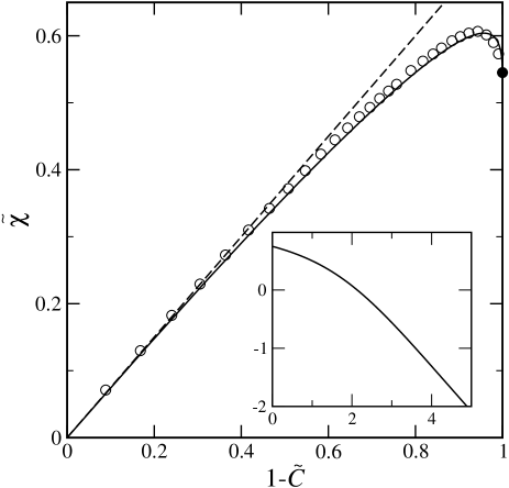
Figure 2: FD-plots for the defect pair observable $A_{1}=n_{i}n_{i+1}$. The full curve shows the limit plot defined by (36), (37). The dashed line has slope $X=\frac{3}{4}$ and is tangent to the limit plot at the origin. The black dot on the right marks the end-point $(1,Y_{1})$ of the limit plot. Simulation data are represented by circles. They are obtained from simulations at $T=0$ in a system of $10^{6}$ spins. The probing field for the susceptibility is $\bar{h}=0.5$ and the data are averaged over 500 runs. In the plot, $t_{\mathrm{w}}=10$ is fixed and $t=10\ldots 15$ is the running parameter. Inset: A plot of the FDR in the short-time regime $X(\Delta t)$, Eq. (31), versus $\Delta t$.

In Fig. 2 the slope of the plot at the origin, where $t_{\mathrm{w}}=t$, is given by $X(0)=\frac{3}{4}$. As $\Delta t$ increases and reaches $\tau^{*}$ the response goes to zero. Consequently the susceptibility reaches a maximum at $\Delta t=\tau^{*}$ and the tangent to the FD-plot in Figure 2 becomes horizontal, with $X(\tau^{*})=0$. As we increase $\Delta t$ further the FDR (31) turns negative and diverges linearly with $\Delta t$, $X(\Delta t)\to-\infty$. Hence the FD-plot becomes vertical as it approaches its end point $(1,Y_{1})$. Taking $\Delta t\to\infty$ in (37), where the integral is solvable Gradshteyn and Ryzhik (2000), gives $Y_{1}=\frac{3}{2}-\frac{3}{\pi}\approx 0.545$. Fluctuation dissipation relations for the aging case, where $\Delta t$ and $t_{\mathrm{w}}$ are comparable, are compressed into this point. So the plot in Figure 2 only reflects the fluctuation dissipation behaviour in the short-time regime. In order to demonstrate that the predicted violation of quasi-equilibrium can easily be observed in simulations we have included such data in Fig. 2.

III.4 Beyond Short Time Differences

Our discussion of the non-equilibrium coarsening dynamics so far was focused on the short-time regime where $\Delta t\geq 0$ finite and $t_{\mathrm{w}}\to\infty$; only the short-time terms $C_{\mathrm{st}},R_{\mathrm{st}}$ in our expressions (22),(23) for the connected two-time defect pair correlation and response functions contributed to leading order in $t_{\mathrm{w}}$. Let us now briefly summarize some interesting features of $C(t,t_{\mathrm{w}})$ and $R(t,t_{\mathrm{w}})$ beyond the short-time regime. Here $\Delta t,t_{\mathrm{w}}\to\infty$ simultaneously, and therefore the aging contributions $C_{\mathrm{ag}},R_{\mathrm{ag}}$, Eqs. (26), (27), must be taken into account.

For correlations we expect to see an effect from the competition between the pair return probability $p_{1}(\Delta t)$ and the chance of finding an independent pair at sites $i,i+1$ at the later time $t$, by analogy with the situation in equilibrium; see Section II.2. In non-equilibrium and for small $\Delta t$ the disconnected and connected correlations coincide to leading order in $t_{\mathrm{w}}$. So from (29) the disconnected correlation is $C^{\mathrm{DC}}(t,t_{\mathrm{w}})\approx D_{1}(t_{\mathrm{w}})p_{1}(t-t_{\mathrm{w}})$. Assuming that this equation applies up to sufficiently large $\Delta t$ – though still much smaller than $t_{\mathrm{w}}$ – we may now estimate the time-scale at which competition sets in. This is done by comparing $C^{\mathrm{DC}}(t,t_{\mathrm{w}})$ to $D_{1}(t_{\mathrm{w}})D_{1}(t)$, which is the product of the independent probabilities of having a defect pair at sites $i,i+1$ at time $t_{\mathrm{w}}$ and at time $t$. Because we are assuming $\Delta t\ll t_{\mathrm{w}}$, $D_{1}(t_{\mathrm{w}})D_{1}(t)\approx D_{1}^{2}(t_{\mathrm{w}})$. The scalings $p_{1}(\Delta t)=O\big{(}\Delta t^{-2}\big{)}$ and $D_{1}(t_{\mathrm{w}})=O\left({t_{\mathrm{w}}}^{-3/2}\right)$ then show that $C^{\mathrm{DC}}(t,t_{\mathrm{w}})$ becomes comparable to $D_{1}(t_{\mathrm{w}})D_{1}(t)$ on the non-trivial time scale $\Delta t=O\left({t_{\mathrm{w}}}^{3/4}\right)$. In fact, from the plots in Fig. 3 the connected correlation becomes negative on that time scale. This means that for $\Delta t\gg{t_{\mathrm{w}}}^{3/4}$, the chances of finding a defect pair at sites $i,i+1$ at time $t$ and at time $t_{\mathrm{w}}$ are lower than those of independently finding pairs at both times: the presence of a defect pair at time $t$ is negatively correlated with that at $t_{\mathrm{w}}$.

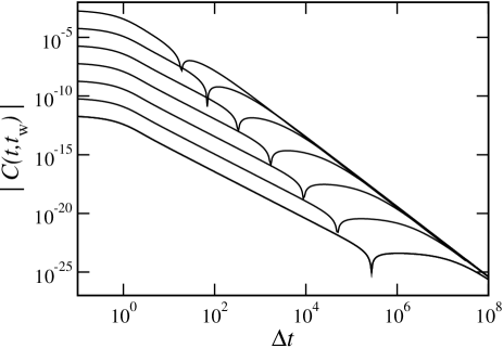
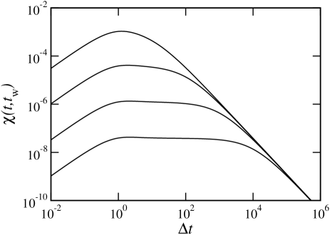
Figure 3: Top: Plots of the exact connected two-time defect pair correlation function $C(t,t_{\mathrm{w}})$ for zero temperature coarsening dynamics, obtained from (22), (24), (26). The curves correspond to $t_{\mathrm{w}}=10^{1},10^{2},\ldots,10^{7}$ from top to bottom, respectively. The cusp in each curve separates the region $C(t,t_{\mathrm{w}})>0$ [at small $\Delta t$] from $C(t,t_{\mathrm{w}})<0$ [at large $\Delta t$]. Bottom: Plots of the exact two-time defect pair susceptibility $\chi(t,t_{\mathrm{w}})$ obtained by numerical integration from (23), (25), (27). The curves correspond to $t_{\mathrm{w}}=10^{1},10^{2},10^{3},10^{4}$ from top to bottom, respectively.

We may picture this effect as follows. If we know that there is a defect pair at sites $i,i+1$ at time $t_{\mathrm{w}}$, the neighboring defects are likely to be at a distance of the order of the typical domain size. Then, as time evolves, the original pair becomes more and more likely to have disappeared via annihilation while neighboring defects have not yet had enough time to reach sites $i,i+1$. For the equilibrium domain size distribution these effects reach a balance on the time-scale $\Delta t=O(\sqrt{\tau_{\mathrm{eq}}})$. In the coarsening case, however, the relative concentration of small domains – as compared to typical domains – is much lower than in equilibrium, so that annihilation of the original pair is comparatively the stronger effect. Thus, on the time-scale $\Delta t=O\left({t_{\mathrm{w}}}^{3/4}\right)$, we have a “hole” in the spatial distribution of defect pairs around sites $i,i+1$. This hole persists up to the time-scale $\Delta t=O(t_{\mathrm{w}})$, where neighboring defects have had time to diffuse in eventually. The connected correlation function, see Fig. 3, therefore has three dynamical regimes at large $t_{\mathrm{w}}$: Up to times $\Delta t\ll{t_{\mathrm{w}}}^{3/4}$ the expansion for the short-time regime (29) applies and $C(t,t_{\mathrm{w}})\sim C_{\mathrm{st}}(t,t_{\mathrm{w}})$. In the time window ${t_{\mathrm{w}}}^{3/4}\ll\Delta t\ll t_{\mathrm{w}}$ the connected correlation is negative and $t$-independent, with contributions from $C_{\mathrm{st}}$ negligible so that $C(t,t_{\mathrm{w}})\sim-D_{1}^{2}(t_{\mathrm{w}})\sim-(1/64)\pi^{-1}t_{\mathrm{w}}^{-3}$. Finally, at large $\Delta t\gg t_{\mathrm{w}}$ the connected correlation remains negative but vanishes as $C(t,t_{\mathrm{w}})\sim-(1/8)\pi^{-1}\Delta t^{-3}$, as follows from expansions of (24), (26).

Comparison of the correlation functions in Fig. 1 and Fig. 3 shows that the simulation data at $t_{\mathrm{w}}=1$ has only given us a glimpse on the full aging behaviour of $C(t,t_{\mathrm{w}})$. From the scales of the plot in Fig. 3, on the other hand, it is clear that such data are out of reach for simulations. Consider, e.g., the curve for $t_{\mathrm{w}}=10^{3}$: the connected correlation $C(t,t_{\mathrm{w}})$ drops from its equal-time value $C(t_{\mathrm{w}},t_{\mathrm{w}})\sim D_{1}(t_{\mathrm{w}})$ of about $10^{-6}$ to around $10^{-12}$, that is by six orders of magnitude, before it deviates from its short-time behaviour $C_{\mathrm{st}}$ and displays aging. This illustrates the general problem associated with exploring the aging behaviour of correlation functions with a scaling of the form (4). We have discussed this issue in the context of single defect observables in the 1$d$ and 2$d$ Ising models in Mayer et al. (2003). There, long-time FD-plots are trivial with $\widetilde{\chi}=1-\widetilde{C}$. However, this only reflects that quasi-equilibrium is satisfied and does not reveal any information about the aging regime. A similar situation is encountered in the 1$d$ FA model which, despite a trivial FD-plot Buhot and Garrahan (2002); Buhot (2003), has $X\neq 1$ in the aging regime Mayer et al. (unpublished). As regards the issue of measuring the asymptotic FDR $X^{\infty}=\lim_{t_{\mathrm{w}}\to\infty}\lim_{t\to\infty}X(t,t_{\mathrm{w}})$, a solution for this problem was suggested in Mayer et al. (2003). It consists in using different observables which share the same $X^{\infty}$ but are more easily accessed in simulations.

The aging behaviour of the two-time defect pair response function $R(t,t_{\mathrm{w}})$ is rather simple. Analysis of (25), (27) shows that the short-time expansion $R(t,t_{\mathrm{w}})\sim R_{\mathrm{st}}(t,t_{\mathrm{w}})$, Eq. (30), applies until $\Delta t$ becomes compareable to $t_{\mathrm{w}}$. More precisely, for $1\ll\Delta t\ll t_{\mathrm{w}}$, we have $R(t,t_{\mathrm{w}})\sim-(3/32)\pi^{-3/2}\Delta t^{-2}{t_{\mathrm{w}}}^{-3/2}$. Note that as discussed in Sec. III.2 the response is negative. In the opposite limit $1\ll t_{\mathrm{w}}\ll\Delta t$ this crosses over to $R(t,t_{\mathrm{w}})\sim-(9/32)\pi^{-3/2}\Delta t^{-3}{t_{\mathrm{w}}}^{-1/2}$, accelerating the decrease of $R(t,t_{\mathrm{w}})$ by a factor of $t_{\mathrm{w}}/\Delta t$. Intuitively speaking, the two defects that were located near sites $i,i+1$ at time $t_{\mathrm{w}}$ and caused the response are likely to have annihilated with other defects in the system when $\Delta t\gg t_{\mathrm{w}}$. This decreases the chances for such a defect pair to return to sites $i,i+1$, and therefore the response.

The scaling of $R(t,t_{\mathrm{w}})$ has an interesting consequence for the susceptibility $\chi(t,t_{\mathrm{w}})=\int_{t_{\mathrm{w}}}^{t}d\tau R(t,\tau)$, also referred to as zero-field-cooled (ZFC) susceptibility. At large $t$ this integral is dominated by the short-time response $R_{\mathrm{st}}$, i.e. $\chi(t,t_{\mathrm{w}})\sim\chi_{\mathrm{st}}(t,t_{\mathrm{w}})$. In the integral, as $\tau$ departs from $t$ the modulus of the integrand $R(t,\tau)$ drops like $(t-\tau)^{-2}$ for $t-\tau\gg 1$ and therefore the integral converges quickly. Aging effects in the scaling of $R(t,\tau)$ when $t-\tau\gg\tau$, i.e. $\tau\ll t/2$, only give small corrections to the value of the integral. Therefore aging contributions in the ZFC susceptibility $\chi(t,t_{\mathrm{w}})$ are subdominant. At large $t$ and for any $t_{\mathrm{w}}\leq t$ this implies $\chi(t,t_{\mathrm{w}})\sim D_{1}(t)\widetilde{\chi}(t-t_{\mathrm{w}})$ with $\widetilde{\chi}$ as given by (37). Consequently we have $\chi(t,t_{\mathrm{w}})\sim Y_{1}D_{1}(t)$ in the aging regime, see Fig. 3, and contributions from aging effects in the response have vanished in $\chi(t,t_{\mathrm{w}})$. We can see the extent of this effect by looking back to Fig. 1: already at the very moderate value of $t_{\mathrm{w}}=1$, aging contributions in $\chi(t,t_{\mathrm{w}})$ are marginal. While all of this is immaterial for exact calculations, where we start from the response in the first place, it is crucial for interpreting simulation results. In problems where the response function has a scaling analogous to (4), see Mayer et al. (2003); Buhot and Garrahan (2002); Buhot (2003), measurement of the ZFC susceptibility gives $\chi(t,t_{\mathrm{w}})\sim\chi_{\mathrm{st}}(t,t_{\mathrm{w}})$ and no information about the aging behaviour of $R(t,t_{\mathrm{w}})$ can be extracted. In a measurement of the so-called thermoremanent (TRM) susceptibility $\rho(t,t_{\mathrm{w}})=\int_{0}^{t_{\mathrm{w}}}d\tau R(t,\tau)$, on the other hand, this bias is not present since $t-\tau\geq t-t_{\mathrm{w}}$. So if $\Delta t>t_{\mathrm{w}}$, for example, the integral only contains contributions from $R(t,\tau)$ with $t-\tau>\tau$ and aging in $R$ is revealed. The situation is precisely reversed as compared to the case of spin observables in critical coarsening Corberi et al. (2003), where the aging behaviour of $R$ can be extracted from $\chi$ but not from $\rho$.

The nonequilibrium FDR $X(t,t_{\mathrm{w}})$ as obtained from (22)-(27) has rather strange features when $\Delta t$ and $t_{\mathrm{w}}$ are simultaneously large. But since the observable $A_{1}$ does not produce quasi-equilibrium FDT in the short-time regime we do not expect $X(t,t_{\mathrm{w}})$ to have a sensible meaning in the context of effective temperatures. We comment only that the short-time expansion (31) applies as long as $\Delta t\ll{t_{\mathrm{w}}}^{3/4}$, while the asymptotic FDR diverges, $X^{\infty}=\infty$.

III.5 Equilibration

Let us finally consider in more detail the crossover to equilibrium for a finite temperature quench $T>0$. We focus again on the short-time regime and, for simplicity, discuss only the equal time FDR $X(t_{\mathrm{w}},t_{\mathrm{w}})$. An expression for $(\partial/\partial t_{\mathrm{w}})C(t,t_{\mathrm{w}})|_{t=t_{\mathrm{w}}}$ is obtained from (55). The instantaneous response $R(t_{\mathrm{w}},t_{\mathrm{w}})$ follows most conveniently from (35) by working out $\widetilde{D}_{1}(t_{\mathrm{w}})$ and $\widetilde{D}_{2}(t_{\mathrm{w}})$ for a quench to $T>0$ Mayer and Sollich (2004). The $t_{\mathrm{w}}$-dependence of the resulting $X(t_{\mathrm{w}},t_{\mathrm{w}})$ for three different temperatures is shown in Figure 4. As expected the curves cross over from $X(t_{\mathrm{w}},t_{\mathrm{w}})=\frac{3}{4}$ at sufficiently small $t_{\mathrm{w}}$ [but still $t_{\mathrm{w}}\gg 1$] to the equilibrium value $X(t_{\mathrm{w}},t_{\mathrm{w}})=1$ at large $t_{\mathrm{w}}$. The time scale for equilibration of $X(t_{\mathrm{w}},t_{\mathrm{w}})$, however, is set by ${\tau_{\mathrm{eq}}}^{2/3}$. In order to understand this result we consider the densities of small domains: in equilibrium we have the scaling $D_{1,\mathrm{eq}}(\tau_{\mathrm{eq}})\sim 1/(2\tau_{\mathrm{eq}})$ whereas for zero temperature coarsening $D_{1}(t_{\mathrm{w}})\sim 1/\left(8\,\sqrt{\pi}\,{t_{\mathrm{w}}}^{3/2}\right)$. This shows that the dynamical density $D_{1}(t_{\mathrm{w}})$ is comparable to the equilibrium density $D_{1,\mathrm{eq}}(\tau_{\mathrm{eq}})$ for $t_{\mathrm{w}}=O\left({\tau_{\mathrm{eq}}}^{2/3}\right)$. By working out $D_{1}=\langle n_{i}n_{i+1}\rangle$ for a quench to $T>0$, one easily verifies that $D_{1}$ indeed becomes stationary at its equilibrium value for $t_{\mathrm{w}}\gg{\tau_{\mathrm{eq}}}^{2/3}$. In this regime one also finds $D_{2}\sim D_{1}$ as expected for low-$T$ equilibrium, rather than $D_{2}\sim 2D_{1}$ in the coarsening regime. From the representation (35) of $R(t_{\mathrm{w}},t_{\mathrm{w}})$ it then follows that the process of defect pair creation starts to contribute to the instantaneous response for $t_{\mathrm{w}}\gg{\tau_{\mathrm{eq}}}^{2/3}$, and that the ratio of the other terms assumes its equilibrium value. It is then not surprising that also the $\Delta t$-dependence of $R(t,t_{\mathrm{w}})$ becomes identical to the equilibrium response throughout the short-time regime, i.e., quasi-equilibrium behavior is recovered for $t_{\mathrm{w}}\gg{\tau_{\mathrm{eq}}}^{2/3}$.

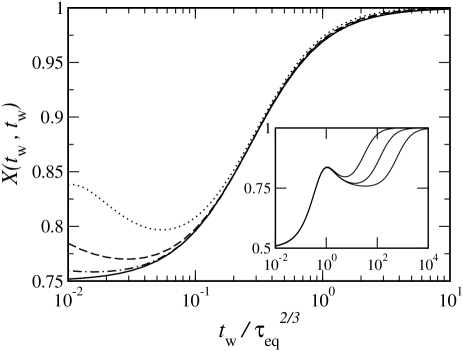
Figure 4: Plots of the equal time FDR $X(t_{\mathrm{w}},t_{\mathrm{w}})$ versus rescaled time $t_{\mathrm{w}}/{\tau_{\mathrm{eq}}}^{2/3}$ for three different temperatures. The curves correspond to $\tau_{\mathrm{eq}}=10^{3}$ (dotted), $\tau_{\mathrm{eq}}=10^{4}$ (dashed) and $\tau_{\mathrm{eq}}=10^{5}$ (dashed-dotted). The full curve applies in the scaling limit $t_{\mathrm{w}},\tau_{\mathrm{eq}}\to\infty$ with $t_{\mathrm{w}}/{\tau_{\mathrm{eq}}}^{2/3}$ fixed. Inset: Plots of $X(t_{\mathrm{w}},t_{\mathrm{w}})$ versus $t_{\mathrm{w}}$ for $\tau_{\mathrm{eq}}=10^{3},10^{4},10^{5}$. The hump at $t_{\mathrm{w}}=1$ is caused by transients following the quench.

IV Non-adjacent defects

In the previous two sections we presented a comprehensive discussion of the functions $C(t,t_{\mathrm{w}})\equiv C_{1}(t,t_{\mathrm{w}})$ and $R(t,t_{\mathrm{w}})\equiv R_{1}(t,t_{\mathrm{w}})$ for the observable $A_{1}=n_{i}n_{i+1}$. Now we investigate to which extent our findings generalize to observables $A_{d}=n_{i}n_{i+d}$ which detect defects a distance $d$ apart. As explained in the Appendix, an exact derivation of the associated functions $C_{d}(t,t_{\mathrm{w}})$ and $R_{d}(t,t_{\mathrm{w}})$ as defined in (5) and (6), respectively, would be extremely cumbersome. Instead we exploit the fact that, in the short-time regime we are interested in, these functions can to leading order in $t_{\mathrm{w}}$ be obtained from random walk arguments.

Consider the states $\boldsymbol{\sigma}$ obtained from low temperature coarsening dynamics at large $t_{\mathrm{w}}$. In complete analogy to the case $d=1$ we have that amongst the states $\boldsymbol{\sigma}$ containing defects at sites $i$ and $i+d$ only a fraction $O\left(t_{\mathrm{w}}^{-3}\right)$ have further defects in any finite neighbourhood. Therefore the discussion of (15) or (29) directly generalizes to any finite $d>1$. In terms of the probability for a defect pair initially located at sites $i,i+d$ to occupy the same sites a time $\Delta t$ later,

$$p_{d}(\Delta t)=G_{\Delta t}(i,i+d;i,i+d),$$ (38)

the correlaton $C_{d}(t,t_{\mathrm{w}})$ in the short-time regime is

$$C_{d}(t,t_{\mathrm{w}})=p_{d}(\Delta t)D_{d}(t_{\mathrm{w}})+O\left(t_{\mathrm{w}}^{-3}\right).$$ (39)

Although this argument applies directly to the disconnected correlations it is also true for $C_{d}(t,t_{\mathrm{w}})$ since both agree to $O\left(D_{d}^{2}\right)=O\left(t_{\mathrm{w}}^{-3}\right)$ in the short time regime. For response functions $R_{d}(t,t_{\mathrm{w}})$ we use (33) and the same reasoning as in Section III.2 to to obtain for $d>1$

$$R_{d} = +\frac{1}{2}\left[G_{\Delta t}(0,d;0,d)-G_{\Delta t}(0,d;0,d-1)\right]D_{d-1}$$ (40)

$$+\frac{1}{2}\left[G_{\Delta t}(0,d;0,d)-G_{\Delta t}(0,d;0,d-1)\right]D_{d}$$

$$+\frac{1}{2}\left[G_{\Delta t}(0,d;0,d)-G_{\Delta t}(0,d;0,d+1)\right]D_{d}$$

$$+\frac{1}{2}\left[G_{\Delta t}(0,d;0,d)-G_{\Delta t}(0,d;0,d+1)\right]D_{d+1}$$

$$+O\left(t_{\mathrm{w}}^{-3}\right).$$

[In order to save space we have omitted here the time arguments $R_{d}=R_{d}(t,t_{\mathrm{w}})$ and $D_{d}=D_{d}(t_{\mathrm{w}})$ etc.] An expression for the $G$’s in (39,40) is stated in (19), giving in particular $p_{d}(\Delta t)=e^{-2\Delta t}\left[I_{0}^{2}-I_{d}^{2}\right](\Delta t)$, while we can estimate $D_{d}(t_{\mathrm{w}})=\widetilde{D}_{d}(t_{\mathrm{w}})+O\left(t_{\mathrm{w}}^{-3}\right)$ using (11).

Before we proceed with a discussion of (39), (40) for nonequilibrium coarsening dynamics, let us briefly consider an equilibrium situation. The above assumption regarding the nature of the states $\boldsymbol{\sigma}$ that contribute to $C_{d}$ and $R_{d}$ then still applies if the temperature is low. Therefore, to leading order in $\tau_{\mathrm{eq}}$, the equivalent of (15) for $d>1$ is $C_{d,\mathrm{eq}}(\Delta t,\tau_{\mathrm{eq}})\sim p_{d}(\Delta t)D_{d,\mathrm{eq}}(\tau_{\mathrm{eq}})$ from (39). In (40), on the other hand, we use $D_{d\pm 1,\mathrm{eq}}(\tau_{\mathrm{eq}})\sim D_{d,\mathrm{eq}}(\tau_{\mathrm{eq}})$ as the density of small domains is flat in low $T$ equilibrium. Combining terms then shows that $R_{d,\mathrm{eq}}(\Delta t,\tau_{\mathrm{eq}})\sim[(-\partial/\partial\Delta t)p_{d}(\Delta t)]D_{d,\mathrm{eq}}(\tau_{\mathrm{eq}})$. Thus equilibrium FDT is recovered from (39), (40) at low temperatures. This is non-trivial because we use zero temperature Glauber rates $w_{n}$ in the derivation of (40), see Section III.2. In contrast to the $d=1$ case of adjacent defects, pair creation processes do not contribute in leading order to the responses $R_{d}$ with $d>1$. This makes sense: the perturbation $\delta\mathcal{H}=-hn_{i}n_{i+d}$ acts on sites a distance $d$ apart but pair creation is only possible on adjacent sites. So the pair creation rate for sites $i+d,i+d+1$ [say] is affected only if we already have a defect present at site $i$. The latter condition makes such contributions in $R_{d}$ subdominant for $d\geq 2$.

Having clarified this qualitative difference between the responses $R_{1}$ and $R_{d}$ with $d\geq 2$ we return to nonequilibrium coarsening dynamics. Here the density of small domains $D_{d}(t_{\mathrm{w}})$ is to leading order proportional to the domain size $d$; more precisely we estimate $D_{d\pm 1}(t_{\mathrm{w}})$ using (11) and $e^{-x}I_{d\pm 1}(x)=e^{-x}I_{d}(x)+O\left(x^{-3/2}\right)$. This allows us to rearrange (40) into

$$R_{d}(t,t_{\mathrm{w}}) = \left[\frac{\partial}{\partial t_{\mathrm{w}}}p_{d}(t-t_{\mathrm{w}})-e^{-2(t-t_{\mathrm{w}})}\frac{I_{d}^{2}(t-t_{\mathrm{w}})}{t-t_{\mathrm{w}}}\right]$$ (41)

$$\times D_{d}(t_{\mathrm{w}})+O\left(t_{\mathrm{w}}^{-5/2}\right).$$

Clearly the nonuniform density of small domains produces a nonequilibrium term in $R_{d}$. It therefore differs from its short-time equilibrium form. From (39), (41) we obtain for the associated FDR in the short-time regime, again abbreviating $X_{d}(\Delta t)=\lim_{t_{\mathrm{w}}\to\infty}X_{d}(t,t_{\mathrm{w}})$,

$$X_{d}(\Delta t)=1-\frac{1}{(-\partial/\partial\Delta t)p_{d}(\Delta t)}e^{-2\Delta t}\frac{I_{d}^{2}(\Delta t)}{\Delta t}.$$ (42)

The equations (39), (41), (42) have a surprising structural similarity with their $d=1$ counter-parts (29), (30), (31). But, in contrast to the case of adjacent defect pairs, $X_{d}(0)=1$ for $d>2$ rather than $X_{1}(0)=\frac{3}{4}$, Eq. 32. From the discussion above we see that effects from perturbing the defect pair creation rate, which are subdominant when $d\geq 2$ but contribute to leading order for $d=1$, are at the origin of this difference. However, it should be stressed that for $\Delta t>0$ all FDRs $X_{d}(\Delta t)$ deviate from unity on an $O(1)$ time-scale. Therefore there is no quasi-equilibrium regime for any defect pair observable $A_{d}$. Instead we have from (42) that $X_{d}(\Delta t)=1-O\left(\Delta t^{2d-1}\right)$ for $\Delta t\ll d^{2}$ while $X_{d}(\Delta t)=-\Delta t/(2d^{2})+O(1)$ for $\Delta t\gg d^{2}$, see Fig. 5.

We visualize the violation of quasi-equilibrium behaviour in terms of FD-plots. The scalings (39) and (40) show that with increasing $t_{\mathrm{w}}$ plots become progressively dominated by the short time behaviour of $C_{d}$ and $R_{d}$. A parameterization of the limit plots is obtained by taking $t_{\mathrm{w}}\to\infty$ at fixed $\Delta t$. Normalizing correlations and susceptibilities as in Section III.3 gives

$$\widetilde{C}_{d} = p_{d}(\Delta t),$$ (43)

$$\widetilde{\chi}_{d} = \left(1-p_{d}(\Delta t)\right)-\int_{0}^{\Delta t}d\tau e^{-2\tau}\frac{I_{d}^{2}(\tau)}{\tau}.$$ (44)

The limit-plots for $d=2,3,4$ are presented in Fig. 5. Each plot has slope $X_{d}(0)=1$ at the origin [not shown] and follows the equilibrium line rather closely until $\Delta t\approx 0.25d^{2}$. Somewhere in the range $2d^{2}<\Delta t<2.5d^{2}$ the plots reach a maximum where $X_{d}=0$, and acquire a vertical tangent as they approach their end points $(1,Y_{d})$, with $X_{d}(\Delta t)\to-\infty$ diverging linearly with $\Delta t$. From (44) the $Y_{d}$ are Gradshteyn and Ryzhik (2000)

$$Y_{d}=1-\frac{2}{\pi d}(-1)^{d}\left[\frac{\pi}{4}+\sum_{k=1}^{d}\frac{(-1)^{k}}{2k-1}\right],$$ (45)

giving $Y_{2}\approx 0.962,Y_{3}\approx 0.983,Y_{4}\approx 0.990$ etc., and $Y_{d}=1-O\left(d^{-2}\right)$ for large $d$. We remark that because the limit plots for $d\geq 2$ lie very close to the equilibrium line – Fig. 5 shows only the top-right corner of the plot – very accurate data would be needed to reproduce them in simulations. Furthermore $\widetilde{\chi}_{d}(t,t_{\mathrm{w}})$ only converges slowly to its $t_{\mathrm{w}}\to\infty$ limit (44). This is easily verified by numerical evaluation of $\widetilde{\chi}_{d}(t,t_{\mathrm{w}})=(1/C(t,t))\int_{t_{\mathrm{w}}}^{t}d\tau R_{d}(t,\tau)$ based on (39), (40). These two facts in combination make it virtually impossible to see the limit plots, Fig. 5, in simulations. Equations (39) and (40), however, perfectly reproduce simulation data for $C_{d}(t,t_{\mathrm{w}})$ and $\chi_{d}(t,t_{\mathrm{w}})=\int_{t_{\mathrm{w}}}^{t}d\tau R_{d}(t,\tau)$ already at small times, e.g., $t_{\mathrm{w}}=10$ and $t=10\ldots 15$ as used in Section III.3.

Our simple random walk analysis does not allow us to make predictions on the aging behaviour of $C_{d}$ and $R_{d}$. If both $\Delta t$ and $t_{\mathrm{w}}$ are large, complicated multi-defect processes must be taken into account; only a calculation as sketched in the Appendix for the case $d=1$ would allow one to study this regime. As regards the susceptibility $\chi_{d}$, however, we can predict that $\chi_{d}(t,t_{\mathrm{w}})\sim Y_{d}D_{d}(t)$ in the aging regime even though we do not know the precise aging behaviour of $R_{d}$. This is simply because $\chi_{d}$ is dominated by the short-time response as discussed in Section III.4.

Finally, for quenches to small but nonzero temperature quasi-equilibrium behaviour will be recovered when $t_{\mathrm{w}}\gg{\tau_{\mathrm{eq}}}^{2/3}$, just as for adjacent defects. This follows from the dependence of the short-time response (40) on the density of small domains $D_{d}$ and $D_{d\pm 1}$ and the fact that these densities level off towards their equilibrium values on that time-scale.

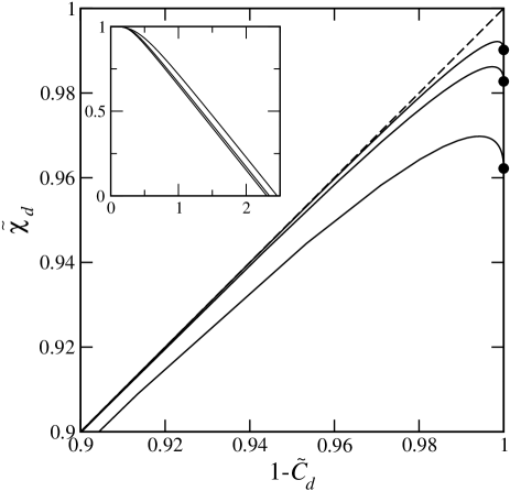
Figure 5: FD limit plots for defect pair observables $A_{d}=n_{i}n_{i+d}$ with $d=2,3,4$ from bottom to top, respectively, obtained from (43), (44). The dashed line has slope $X=1$ and represents equilibrium FDT. Black dots mark the end-points $(1,Y_{d})$ of the limit plots. Inset: Plots of the FDRs in the short-time regime $X_{d}(\Delta t)$, Eq. (42), with $d=2,3,4$ from top to bottom, respectively, versus $\Delta t/d^{2}$. The curves for $d=3,4$ are almost indistinguishable, showing that $X_{d}$ quickly approaches a scaling form.

V Conclusions

In this paper we have analyzed the FDT behavior for defect-pair observables $A_{d}=n_{i}n_{i+d}$ in the Glauber-Ising chain. Contrary to the commonly held notion that short-time relaxation generally proceeds as if in equilibrium, none of these observables produce $X=1$ in the short-time regime $\Delta t\ll t_{\mathrm{w}}$; this applies as long as $t_{\mathrm{w}}$ is below the crossover timescale ${\tau_{\mathrm{eq}}}^{2/3}$. We showed explicitly that this unusual behavior arises from the response functions, while the short-time decay of correlations does indeed have an equilibrium form apart from the expected overall amplitude factor. The deviations of the responses from quasi-equilibrium behavior could be traced to two factors. First, in the out-of-equilibrium response for adjacent defects, events where pairs of domain walls are created are negligible, while in equilibrium they contribute at leading order. Second, all responses are sensitive to details of the domain-size distribution in the system, via their dependence on the density of small domains, and these details differ between the equilibrium and out-of-equilibrium situations.

The inherent-structure picture mentioned in the introduction suggests a generic interpretation of our results: starting from an out-of-equilibrium configuration with a given number of defects or domain walls, we can loosely say that we remain within the same “basin” as long as no domain walls annihilate; the energy then remains constant. A similar interpretation has been advocated, in the context of the Fredrickson-Andersen model, in Berthier and Garrahan (2003). Transitions to a basin with lower energy then correspond to the annihilation of two domain walls; at long coarsening times $t_{\mathrm{w}}$, such transitions between basins are separated by long stretches of “intra-basin” motion. Within this picture, our defect-pair observables $A_{d}$ measure precisely when a transition to a new basin is about to happen, i.e., they focus on the out-of-equilibrium, inter-basin dynamics. From this point of view it is not surprising that the $A_{d}$ do not exhibit quasi-equilibrium behavior even at short times. Spin and single-defect observables, on the other hand, are not unusually sensitive to transitions between basins, so that their short-time relaxation is governed by the quasi-equilibrium, intra-basin motion Mayer et al. (2003); Buhot and Garrahan (2002); Buhot (2003). This highlights the crucial dependence of nonequilibrium fluctuation-dissipation relations on the probing observables.

The above interpretation suggests that lack of quasi-equilibrium behavior in the short-time regime could occur quite generically in glassy systems. Certainly in glass models with kinetically constrained dynamics Ritort and Sollich (2003), one would expect observables that detect the proximity of two or more facilitating defects to display similar behaviour to the one studied in this paper. More generally, the same should apply to observables which are sensitive to transitions between basins or metastable states. In structural glasses, conventional observables such as density fluctuations are clearly not of this type. However, observables which measure, e.g., how close a local particle configuration is to rearranging into a different local structure could be expected to display violations of quasi-equilibrium behavior. If the density of such configurations decreases with increasing $t_{\mathrm{w}}$ then the bound of Cugliandolo et al. (1997b) is essentially void as discussed below Eq. (2). It would be interesting to construct such observables explicitly – thresholding of an appropriately defined free volume would seem an obvious candidate – and to test our hypothesis in simulations.

Finally, the requirement that the short-time relaxation should display quasi-equilibrium behavior could be used to narrow down the class of “neutral observables” which are suitable for measuring a well-defined effective temperature in the limit of large time differences. We note in this context that the condition $\lim_{t_{\mathrm{w}}\to\infty}(\partial/\partial t_{\mathrm{w}})C(t,t_{\mathrm{w}})\neq 0$ at fixed $\Delta t$ is not necessary to obtain quasi-equilibrium FDT. For the single-defect observables considered in Mayer et al. (2003); Buhot and Garrahan (2002); Buhot (2003), for instance, this limit vanishes yet quasi-equilibrium behavior is observed nevertheless.

*

Appendix A

We summarize below the ingredients that are needed to obtain our expressions for $C\equiv C_{1}$ and $R\equiv R_{1}$ based on the general results derived in Mayer and Sollich (2004). The correlation $C(t,t_{\mathrm{w}})$ is first reduced to multispin correlations by substituting $n_{i}=\frac{1}{2}\left(1-\sigma_{i}\sigma_{i+1}\right)$ in (5). This gives

$$16\,C(t,t_{\mathrm{w}}) = +C_{(0,1),(0,1)}+C_{(0,1),(1,2)}-C_{(0,1),(0,2)}$$

$$+C_{(1,2),(0,1)}+C_{(1,2),(1,2)}-C_{(1,2),(0,2)}$$

$$-C_{(0,2),(0,1)}-C_{(0,2),(1,2)}+C_{(0,2),(0,2)},$$

where

$$C_{\boldsymbol{i},\boldsymbol{j}} = \langle\sigma_{i_{1}}(t)\sigma_{i_{2}}(t)\sigma_{j_{1}}(t_{\mathrm{w}})\sigma_{j_{2}}(t_{\mathrm{w}})\rangle$$ (46)

$$-\langle\sigma_{i_{1}}(t)\sigma_{i_{2}}(t)\rangle\langle\sigma_{j_{1}}(t_{\mathrm{w}})\sigma_{j_{2}}(t_{\mathrm{w}})\rangle.$$

We have omitted the time-arguments in $C_{\boldsymbol{i},\boldsymbol{j}}$ in order to save space. When using the symmetries of $C_{\boldsymbol{i},\boldsymbol{j}}$ under translations, reflections and permutations [among the components of $\boldsymbol{i}$ and $\boldsymbol{j}$ but not between $\boldsymbol{i}$ and $\boldsymbol{j}$] the above equation for $C(t,t_{\mathrm{w}})$ assumes the simpler form

$$C(t,t_{\mathrm{w}}) = \frac{1}{8}\left[C_{(0,1),(0,1)}+C_{(1,2),(0,1)}-C_{(0,1),(0,2)}\right.$$ (47)

$$\left.-C_{(0,2),(0,1)}\right]+\frac{1}{16}C_{(0,2),(0,2)}.$$

Note that while $C(t,t_{\mathrm{w}})$ can be expressed in terms of 4-spin correlations (46) only, this is not possible for $d\geq 2$; in the latter case the expressions for $C_{d}(t,t_{\mathrm{w}})$ contain 8-spin two-time correlations and exact calculations become exceedingly cumbersome. In full analogy to $C(t,t_{\mathrm{w}})$ the response $R$ may be decomposed into

$$R(t,t_{\mathrm{w}}) = \frac{1}{8}\left[R_{(0,1),(0,1)}+R_{(1,2),(0,1)}-R_{(0,1),(0,2)}\right.$$ (48)

$$\left.-R_{(0,2),(0,1)}\right]+\frac{1}{16}R_{(0,2),(0,2)},$$

with

$$R_{\boldsymbol{i},\boldsymbol{j}}=T\left.\frac{\delta\langle\sigma_{i_{1}}(t)\sigma_{i_{2}}(t)\rangle}{\delta h_{\boldsymbol{j}}(t_{\mathrm{w}})}\right|_{h_{\boldsymbol{j}}=0}.$$ (49)

For the multispin response function (49) the field $h_{\boldsymbol{j}}$ is thermodynamically conjugate to $\sigma_{j_{1}}\sigma_{j_{2}}$. Let us remark that while the pair $C$, $R$ violates quasi-equilibrium this is not the case  for the constituting pairs $C_{\boldsymbol{i},\boldsymbol{j}}$, $R_{\boldsymbol{i},\boldsymbol{j}}$. Next, the 4-spin correlations in (47) are expressed in terms of the result given in Mayer and Sollich (2004), viz.,

$$C_{\boldsymbol{i},\boldsymbol{j}} = +\big{[}\mathcal{F}_{i_{1},i_{2}}^{\,\boldsymbol{j}}-H_{i_{2}-i_{1}}(2\Delta t,2t_{\mathrm{w}})\big{]}\,H_{j_{2}-j_{1}}(2t_{\mathrm{w}})$$ (50)

$$-\big{[}+e^{-\Delta t}\,I_{i_{1}-j_{1}}(\gamma\Delta t)+\mathcal{E}_{i_{1},j_{1}}^{\,\boldsymbol{j}}\big{]}$$

$$\times\big{[}-e^{-\Delta t}\,I_{i_{2}-j_{2}}(\gamma\Delta t)+\mathcal{E}_{i_{2},j_{2}}^{\,\boldsymbol{j}}\big{]}$$

$$+\big{[}-e^{-\Delta t}\,I_{i_{1}-j_{2}}(\gamma\Delta t)+\mathcal{E}_{i_{1},j_{2}}^{\,\boldsymbol{j}}\big{]}$$

$$\times\big{[}+e^{-\Delta t}\,I_{i_{2}-j_{1}}(\gamma\Delta t)+\mathcal{E}_{i_{2},j_{1}}^{\,\boldsymbol{j}}\big{]}.$$

Here and below the indices $\boldsymbol{i}=(i_{1},i_{2})$ and $\boldsymbol{j}=(j_{1},j_{2})$ must satisfy $i_{1}<i_{2}$ and $j_{1}<j_{2}$. The multispin response function (49) for the case $j_{2}=j_{1}+1$ is also stated explicitly in Mayer and Sollich (2004) and reads [$\boldsymbol{j}^{1,\mathrm{s}}=(j_{1}-1,j_{1})$ and $\boldsymbol{j}^{2,\mathrm{s}}=(j_{2},j_{2}+1)$]

$$R_{\boldsymbol{i},\boldsymbol{j}} = +e^{-\Delta t}\,I_{i_{1}-j_{1}}\left[-\left(1-\frac{\gamma^{2}}{2}\right)\left(-e^{-\Delta t}\,I_{i_{2}-j_{2}}+\mathcal{E}_{i_{2},j_{2}}^{\,\boldsymbol{j}}\right)+\frac{\gamma^{2}}{2}\left(+e^{-\Delta t}\,I_{i_{2}-j_{1}+1}+\mathcal{E}_{i_{2},j_{1}-1}^{\,\boldsymbol{j}^{1,\mathrm{s}}}\right)\right]$$ (51)

$$+e^{-\Delta t}\,I_{i_{2}-j_{1}}\left[+\left(1-\frac{\gamma^{2}}{2}\right)\left(-e^{-\Delta t}\,I_{i_{1}-j_{2}}+\mathcal{E}_{i_{1},j_{2}}^{\,\boldsymbol{j}}\right)-\frac{\gamma^{2}}{2}\left(+e^{-\Delta t}\,I_{i_{1}-j_{1}+1}+\mathcal{E}_{i_{1},j_{1}-1}^{\,\boldsymbol{j}^{1,\mathrm{s}}}\right)\right]$$

$$-e^{-\Delta t}\,I_{i_{1}-j_{2}}\left[+\left(1-\frac{\gamma^{2}}{2}\right)\left(+e^{-\Delta t}\,I_{i_{2}-j_{1}}+\mathcal{E}_{i_{2},j_{1}}^{\,\boldsymbol{j}}\right)-\frac{\gamma^{2}}{2}\left(-e^{-\Delta t}\,I_{i_{2}-j_{2}-1}+\mathcal{E}_{i_{2},j_{2}+1}^{\,\boldsymbol{j}^{2,\mathrm{s}}}\right)\right]$$

$$-e^{-\Delta t}\,I_{i_{2}-j_{2}}\left[-\left(1-\frac{\gamma^{2}}{2}\right)\left(+e^{-\Delta t}\,I_{i_{1}-j_{1}}+\mathcal{E}_{i_{1},j_{1}}^{\,\boldsymbol{j}}\right)+\frac{\gamma^{2}}{2}\left(-e^{-\Delta t}\,I_{i_{1}-j_{2}-1}+\mathcal{E}_{i_{1},j_{2}+1}^{\,\boldsymbol{j}^{2,\mathrm{s}}}\right)\right].$$

We have omitted the arguments $(\gamma\Delta t)$ of the functions $I$ in order to save space. The multispin response functions for the case $j_{2}>j_{1}+1$ are not given explicitly in Mayer and Sollich (2004). However, by following the general procedure developed there one verifies the result [$\boldsymbol{j}^{1,\mathrm{s}}=(j_{1}-1,j_{1},j_{1}+1,j_{2})$ and $\boldsymbol{j}^{2,\mathrm{s}}=(j_{1},j_{2}-1,j_{2},j_{2}+1)$]

$$R_{\boldsymbol{i},\boldsymbol{j}} = +e^{-\Delta t}\,I_{i_{1}-j_{1}}\bigg{\{}\!-\left(1-\frac{\gamma^{2}}{2}\right)\left(-e^{-\Delta t}\,I_{i_{2}-j_{2}}+\mathcal{E}_{i_{2},j_{2}}^{\,\boldsymbol{j}}\right)+\frac{\gamma^{2}}{2}\Big{[}\left(+e^{-\Delta t}\,I_{i_{2}-j_{1}+1}+\mathcal{E}_{i_{2},j_{1}-1}^{\,\boldsymbol{j}^{1,\mathrm{s}}}\right)H_{j_{2}-j_{1}-1}$$ (52)

$$\qquad-\left(+e^{-\Delta t}\,I_{i_{2}-j_{1}-1}+\mathcal{E}_{i_{2},j_{1}+1}^{\,\boldsymbol{j}^{1,\mathrm{s}}}\right)H_{j_{2}-j_{1}+1}+\left(-e^{-\Delta t}\,I_{i_{2}-j_{2}}+\mathcal{E}_{i_{2},j_{2}}^{\,\boldsymbol{j}^{1,\mathrm{s}}}\right)H_{2}\Big{]}\bigg{\}}$$

$$+e^{-\Delta t}\,I_{i_{2}-j_{1}}\bigg{\{}\!+\left(1-\frac{\gamma^{2}}{2}\right)\left(-e^{-\Delta t}\,I_{i_{1}-j_{2}}+\mathcal{E}_{i_{1},j_{2}}^{\,\boldsymbol{j}}\right)-\frac{\gamma^{2}}{2}\Big{[}\left(+e^{-\Delta t}\,I_{i_{1}-j_{1}+1}+\mathcal{E}_{i_{1},j_{1}-1}^{\,\boldsymbol{j}^{1,\mathrm{s}}}\right)H_{j_{2}-j_{1}-1}$$

$$\qquad-\left(+e^{-\Delta t}\,I_{i_{1}-j_{1}-1}+\mathcal{E}_{i_{1},j_{1}+1}^{\,\boldsymbol{j}^{1,\mathrm{s}}}\right)H_{j_{2}-j_{1}+1}+\left(-e^{-\Delta t}\,I_{i_{1}-j_{2}}+\mathcal{E}_{i_{1},j_{2}}^{\,\boldsymbol{j}^{1,\mathrm{s}}}\right)H_{2}\Big{]}\bigg{\}}$$

$$-e^{-\Delta t}\,I_{i_{1}-j_{2}}\bigg{\{}\!+\left(1-\frac{\gamma^{2}}{2}\right)\left(+e^{-\Delta t}\,I_{i_{2}-j_{1}}+\mathcal{E}_{i_{2},j_{1}}^{\,\boldsymbol{j}}\right)-\frac{\gamma^{2}}{2}\Big{[}\left(+e^{-\Delta t}\,I_{i_{2}-j_{1}}+\mathcal{E}_{i_{2},j_{1}}^{\,\boldsymbol{j}^{2,\mathrm{s}}}\right)H_{2}$$

$$\qquad-\left(-e^{-\Delta t}\,I_{i_{2}-j_{2}+1}+\mathcal{E}_{i_{2},j_{2}-1}^{\,\boldsymbol{j}^{2,\mathrm{s}}}\right)H_{j_{2}-j_{1}+1}+\left(-e^{-\Delta t}\,I_{i_{2}-j_{1}-1}+\mathcal{E}_{i_{2},j_{2}+1}^{\,\boldsymbol{j}^{2,\mathrm{s}}}\right)H_{j_{2}-j_{1}-1}\Big{]}\bigg{\}}$$

$$-e^{-\Delta t}\,I_{i_{2}-j_{2}}\bigg{\{}\!-\left(1-\frac{\gamma^{2}}{2}\right)\left(+e^{-\Delta t}\,I_{i_{1}-j_{1}}+\mathcal{E}_{i_{1},j_{1}}^{\,\boldsymbol{j}}\right)+\frac{\gamma^{2}}{2}\Big{[}\left(+e^{-\Delta t}\,I_{i_{1}-j_{1}}+\mathcal{E}_{i_{1},j_{1}}^{\,\boldsymbol{j}^{2,\mathrm{s}}}\right)H_{2}$$

$$\qquad-\left(-e^{-\Delta t}\,I_{i_{1}-j_{2}+1}+\mathcal{E}_{i_{1},j_{2}-1}^{\,\boldsymbol{j}^{2,\mathrm{s}}}\right)H_{j_{2}-j_{1}+1}+\left(-e^{-\Delta t}\,I_{i_{1}-j_{2}-1}+\mathcal{E}_{i_{1},j_{2}+1}^{\,\boldsymbol{j}^{2,\mathrm{s}}}\right)H_{j_{2}-j_{1}-1}\Big{]}\bigg{\}}.$$

Again, all functions $I$ have argument $(\gamma\Delta t)$ and additionally all functions $H$ appearing in (52) have argument $(2t_{\mathrm{w}})$. After substituting (50), (51), (52) for the multispin correlation and response functions in (47) and (48), $C(t,t_{\mathrm{w}})$ and $R(t,t_{\mathrm{w}})$ are expressed in terms of $I,H,\mathcal{E}$ and $\mathcal{F}$. Next we also represent $\mathcal{E}$ and $\mathcal{F}$ in terms of $I$ and $H$ by applying the corresponding formulas derived in Mayer and Sollich (2004), viz.

$$\mathcal{E}_{i_{\varepsilon},j_{\nu}}^{\,\boldsymbol{j}} = H_{j_{\nu}-i_{\varepsilon}}(\Delta t,2t_{\mathrm{w}})$$

$$-\sum_{m}\boldsymbol{\delta}_{\boldsymbol{j},m}\,e^{-\Delta t}\,I_{i_{\varepsilon}-m}(\gamma\Delta t)\,H_{j_{\nu}-m}(2t_{\mathrm{w}}),$$

and

$$\mathcal{F}_{i_{\varepsilon},i_{\delta}}^{\,\boldsymbol{j}} = H_{i_{\delta}-i_{\varepsilon}}(2\Delta t,2t_{\mathrm{w}})$$

$$-\sum_{m}\boldsymbol{\delta}_{\boldsymbol{j},m}\,e^{-\Delta t}I_{i_{\varepsilon}-m}(\gamma\Delta t)\,H_{i_{\delta}-m}(\Delta t,2t_{\mathrm{w}})$$

$$+\sum_{m}\boldsymbol{\delta}_{\boldsymbol{j},m}\,e^{-\Delta t}I_{i_{\delta}-m}(\gamma\Delta t)\,H_{i_{\varepsilon}-m}(\Delta t,2t_{\mathrm{w}})$$

$$+\sum_{m,n}\boldsymbol{\delta}_{\boldsymbol{j},m}\,\boldsymbol{\delta}_{\boldsymbol{j},n}\,e^{-2\Delta t}\,I_{i_{\varepsilon}-m}(\gamma\Delta t)\,I_{i_{\delta}-n}(\gamma\Delta t)$$

$$\times H_{n-m}(2t_{\mathrm{w}}),$$

where $\boldsymbol{\delta}_{\boldsymbol{j},m}=1-\mathrm{sgn}(j_{1}-m)\cdots\mathrm{sgn}(j_{p}-m)$ with $p=\mathrm{dim}(\boldsymbol{j})$, i.e. $p=2$ or 4 in our case. The sums in these equations are finite since $\boldsymbol{\delta}_{\boldsymbol{j},m}$ is nonzero only within the index-range covered by the components of $\boldsymbol{j}$. Upon substitution of the latter equations for all functions $\mathcal{E}$, $\mathcal{F}$ the defect-pair correlation and response functions are expressed purely in terms of $I,H$. The functions $H$, in turn, are expressed in terms of modified Bessel functions via

$$H_{n}(t_{1},t_{2})=\frac{\gamma}{2}\int_{t_{1}}^{t_{1}+t_{2}}d\tau\,e^{-\tau}\left[I_{n-1}-I_{n+1}\right](\gamma\tau),$$ (53)

where we use the notation $H_{n}(\tau)=H_{n}(0,\tau)$. In equilibrium the quantity $H_{n,\mathrm{eq}}(\tau)=\lim_{t\to\infty}H_{n}(\tau,t)$ is relevant, cf. Eq. 12. Simplification of the expressions for $C$ and $R$ are possible when using the recursion formula

$$H_{n+1}(t_{1},t_{2}) = -H_{n-1}(t_{1},t_{2})+\frac{2}{\gamma}\,H_{n}(t_{1},t_{2})$$ (54)

$$+e^{-t_{1}-t_{2}}\left[I_{n-1}-I_{n+1}\right]\left(\gamma(t_{1}+t_{2})\right)$$

$$-e^{-t_{1}}\left[I_{n-1}-I_{n+1}\right]\left(\gamma t_{1}\right).$$

One easily proves (54) when substituting (53) and integrating by parts. With $H_{0}(t_{1},t_{2})=0$, which follows trivially from (53), any function $H_{n}(t_{1},t_{2})$ may thus be decomposed into modified Bessel functions and $H_{1}(t_{1},t_{2})$. Also, the recursion $[I_{n-1}-I_{n+1}](x)=\frac{2n}{x}I_{n}(x)$ is useful for rearranging the results. We use Mathematica 5.0 to carry out the algebraic manipulations described above. The procedure yields significant cancellations in the expressions for $C$ and $R$. For a quench to $T>0$ we obtain (55), see below, and a similar expression for $R$; taking $T\to 0$ where the integral $H_{1}$ is soluble Mayer and Sollich (2004) then produces the results (22)-(27).

$$C(t,t_{\mathrm{w}}) \!\!=\!\! -\frac{1}{4\gamma^{2}}\bigg{\{}e^{-(t+t_{\mathrm{w}})}\frac{I_{1}(\gamma(t+t_{\mathrm{w}}))}{t+t_{\mathrm{w}}}\bigg{[}e^{-(t+t_{\mathrm{w}})}\frac{I_{1}(\gamma(t+t_{\mathrm{w}}))}{t+t_{\mathrm{w}}}-2\gamma e^{-(t-t_{\mathrm{w}})}[I_{0}-I_{1}](\gamma(t-t_{\mathrm{w}}))[1-H_{1}(2t_{\mathrm{w}})]\bigg{]}$$ (55)

$$+H_{1}(t-t_{\mathrm{w}},2t_{\mathrm{w}})\bigg{[}\frac{2}{\tau_{\mathrm{eq}}}e^{-(t+t_{\mathrm{w}})}\frac{I_{1}(\gamma(t+t_{\mathrm{w}}))}{t+t_{\mathrm{w}}}-2\gamma e^{-(t-t_{\mathrm{w}})}[I_{0}-I_{1}](\gamma(t-t_{\mathrm{w}}))\bigg{(}\frac{1}{\tau_{\mathrm{eq}}}+e^{-2t_{\mathrm{w}}}\frac{I_{1}(2\gamma t_{\mathrm{w}})}{2t_{\mathrm{w}}}\bigg{)}\bigg{]}$$

$$+\frac{1}{{\tau_{\mathrm{eq}}}^{2}}H_{1}^{2}(t-t_{\mathrm{w}},2t_{\mathrm{w}})\bigg{\}}.$$

References

• Stillinger and Weber (1984) F. H. Stillinger and T. A. Weber, Science 225, 983 (1984).
• Cugliandolo and Kurchan (1993) L. F. Cugliandolo and J. Kurchan, Phys. Rev. Lett. 71, 173 (1993).
• Cugliandolo et al. (1997a) L. F. Cugliandolo, J. Kurchan, and L. Peliti, Phys. Rev. E 55, 3898 (1997a).
• Crisanti and Ritort (2003) A. Crisanti and F. Ritort, J. Phys. A: Math. Gen. 36, 181 (2003).
• Cugliandolo et al. (1997b) L. F. Cugliandolo, D. S. Dean, and J. Kurchan, Phys. Rev. Lett. 79, 2168 (1997b).
• Bouchaud et al. (1998) J. P. Bouchaud, L. F. Cugliandolo, J. Kurchan, and M. Mézard, in Spin glasses and random fields, edited by A. P. Young (World Scientific, Singapore, 1998).
• Godrèche and Luck (2002) C. Godrèche and J. M. Luck, J. Phys.: Cond-Mat 14, 1589 (2002).
• Götze and Sjögren (1992) W. Götze and L. Sjögren, Rep. Prog. Phys. 55, 241 (1992).
• Mayer et al. (2003) P. Mayer, L. Berthier, J. P. Garrahan, and P. Sollich, Phys. Rev. E 68, 016116 (2003).
• Buhot and Garrahan (2002) A. Buhot and J. P. Garrahan, Phys. Rev. Lett. 88, 225702 (2002).
• Buhot (2003) A. Buhot, J. Phys. A-Math. Gen. 36, 12367 (2003).
• Sastre et al. (2003) F. Sastre, I. Dornic, and H. Chate, Phys. Rev. Lett. 91, 267205 (2003).
• Berthier and Barrat (2002a) L. Berthier and J. L. Barrat, Phys. Rev. Lett. 89, 095702 (2002a).
• Berthier and Barrat (2002b) L. Berthier and J. L. Barrat, J. Chem. Phys. 116, 6228 (2002b).
• Fielding and Sollich (2002) S. Fielding and P. Sollich, Phys. Rev. Lett. 88, 050603 (2002).
• Sollich et al. (2002) P. Sollich, S. Fielding, and P. Mayer, J. Phys.-Cond. Mat. 14, 1683 (2002).
• Godrèche and Luck (2000) C. Godrèche and J. M. Luck, J. Phys. A: Math. Gen. 33, 1151 (2000).
• Lippiello and Zannetti (2000) E. Lippiello and M. Zannetti, Phys. Rev. E 61, 3369 (2000).
• Glauber (1963) R. J. Glauber, J. Math. Phys. 4, 294 (1963).
• Derrida and Zeitak (1996) B. Derrida and R. Zeitak, Phys. Rev. E 54, 2513 (1996).
• Mayer and Sollich (2004) P. Mayer and P. Sollich, J. Phys. A: Math. Gen. 37, 9 (2004).
• Gradshteyn and Ryzhik (2000) L. S. Gradshteyn and I. M. Ryzhik, Table of Integrals, Series, and Products (Academic Press, New York, 2000).
• Alemany and Benavraham (1995) P. A. Alemany and D. Benavraham, Phys. Lett. A 206, 18 (1995).
• Santos (1997) J. E. Santos, J. Phys. A-Math. Gen. 30, 3249 (1997).
• Barrat (1998) A. Barrat, Phys. Rev. E 57, 3629 (1998).
• Bortz et al. (1975) A. B. Bortz, M. H. Kalos, and J. L. Lebowitz, J. Comput. Phys. 17, 10 (1975).
• Mayer et al. (2004) P. Mayer, L. Berthier, J. P. Garrahan, and P. Sollich, Phys. Rev. E 70, 018102 (2004).
• Mayer et al. (unpublished) P. Mayer, L. Berthier, J. P. Garrahan, and P. Sollich (unpublished).
• Corberi et al. (2003) F. Corberi, E. Lippiello, and M. Zannetti, Phys. Rev. E 68, 046131 (2003).
• Berthier and Garrahan (2003) L. Berthier and J. P. Garrahan, J. Chem. Phys. 119, 4367 (2003).
• Ritort and Sollich (2003) F. Ritort and P. Sollich, Adv. Phys. 52, 219 (2003).