Work and heat fluctuations in two-state systems: a trajectory thermodynamics formalism

Abstract

Two-state models provide phenomenological descriptions of many different systems, ranging from physics to chemistry and biology. We investigate work fluctuations in an ensemble of two-state systems driven out of equilibrium under the action of an external perturbation. We calculate the probability density $P_{N}(W)$ that a work equal to $W$ is exerted upon the system (of size $N$) along a given non-equilibrium trajectory and introduce a trajectory thermodynamics formalism to quantify work fluctuations in the large-$N$ limit. We then define a trajectory entropy $S_{N}(W)$ that counts the number of non-equilibrium trajectories $P_{N}(W)=\exp(S_{N}(W)/k_{B}T)$ with work equal to $W$ and characterizes fluctuations of work trajectories around the most probable value $W^{\rm mp}$. A trajectory free-energy ${\cal F}_{N}(W)$ can also be defined, which has a minimum at $W=W^{{\dagger}}$, this being the value of the work that has to be efficiently sampled to quantitatively test the Jarzynski equality. Within this formalism a Lagrange multiplier is also introduced, the inverse of which plays the role of a trajectory temperature. Our general solution for $P_{N}(W)$ exactly satisfies the fluctuation theorem by Crooks and allows us to investigate heat-fluctuations for a protocol that is invariant under time reversal. The heat distribution is then characterized by a Gaussian component (describing small and frequent heat exchange events) and exponential tails (describing the statistics of large deviations and rare events). For the latter, the width of the exponential tails is related to the aforementioned trajectory temperature. Finite-size effects to the large-$N$ theory and the recovery of work distributions for finite $N$ are also discussed. Finally, we pay particular attention to the case of magnetic nanoparticle systems under the action of a magnetic field $H$ where work and heat fluctuations are predicted to be observable in ramping experiments in micro-SQUIDs.

1 Introduction

There has been recent interest in the experimental measure of work fluctuations and the test of the so-called fluctuation theorems. Initially proposed in the context of sheared systems in a steady state [1] several versions of such theorems have been derived [2]. In particular, specific identities have been obtained in the context of stochastic systems that show how it is possible to recover the equilibrium free-energy change in a reversible transformation by exponential averaging over many non-equilibrium trajectories that start at equilibrium [3, 4, 5]. Let us consider a system initially in equilibrium in contact with a thermal bath (at temperature $T$) that is submitted to an isothermal perturbation according to a given protocol. Work fluctuations (WF) refer to the fact that the work $W$ exerted upon the system depends on the particular non-equilibrium trajectory followed by the system. As the initial configuration or the trajectory are stochastic, the value of the work $W$ changes among different trajectories, all generated with the same perturbation protocol. Transient violations (TV) of the second law refer to the fact that, among all possible WF, a fraction of them absorb heat from the bath that is transformed into work. Taken individually, these rare trajectories violate the Clausius inequality, $Q\leq T\Delta S$, where $Q$ is the heat supplied from the bath to the system and $\Delta S$ is the change in the entropy, a state function defined through the transformation. In a transformation cycle $\Delta S=0$ these TV satisfy $Q>0$ i.e., they can absorb a net amount of heat from the bath during the cycle. In terms of the dissipated work $W_{\rm dis}$, the Clausius relation can be expressed in the following form,

$$W_{\rm dis}=W-W_{\rm rev}=T\Delta S-Q\geq 0$$ (1)

In this expression $W$ is the total work exerted upon the system. According to the first law of thermodynamics (conservation of the energy) $W$ is given by $W=\Delta E-Q$ where $\Delta E$ is the change in the internal energy, $W_{\rm rev}$ is the reversible work (identical to the free-energy change $\Delta F=\Delta E-T\Delta S$). Both the heat $Q$ and $W_{\rm dis}$ (or $W$) are trajectory dependent, however $\Delta S$ and $W_{\rm rev}$ are both trajectory independent as they are state functions, only dependent on the initial and final states. The Clausius inequality (1) has to be understood as a result that is valid after averaging the fluctuating quantities $Q$ and $W$ over an infinite number of trajectories (in what follows we will denote this average by $\overline{(..)}$). The second law reads $\overline{W_{\rm dis}}\geq 0$ and TV of the second law refer to the existence of trajectories where $W_{\rm dis}<0$. From this point of view, TV are just WF characterized by the fact that $W_{\rm dis}<0$. The interest in studying TV is that these describe large deviations of the work that have to be sampled in order to recover equilibrium free-energy differences from non-equilibrium measurements [6].

The steadily increasing development of nanotechnologies during the last decade has made WF experimentally accessible. Recent experiments on single RNA hairpins unfolded under the action of mechanical force [7] and micro-sized beads trapped by laser tweezers and moved through a solvent [8] have provided a first quantitative estimate of WF and TV. Related measurements include the experimental verification of the Gallavotti-Cohen fluctuation theorem in Rayleigh-Bernard convection [9] and turbulent flows [10]. This research is potentially very interesting as it leads to new insights about the physical processes occurring at the nanoscale, a frontier that marks the onset of complex organization of matter [11]. A characteristic of WF is that they are quickly suppressed as the system size or the time window of the measurement increase.

The central quantity describing WF is the work probability distribution $P_{N}(W)$ ($N$ stands for the system size), $P_{N}(W)dW$ being the fraction of non-equilibrium trajectories with work between $W$ and $W+dW$. The knowledge of this quantity is important for what it tells us about the mathematical form of the tails of the distribution, relevant to understand the importance of large deviations of work values respect to the average value. A precise knowledge of the form of the tails in that distribution gives us hints about how many experiments need to be done in order to recover equilibrium quantities from non-equilibrium experiments. In this work we investigate an ensemble of two-level systems as an explicit example where $P_{N}(W)$ can be analytically computed in the large-$N$ approach using a path integral method. This approach allows us to exactly derive several exact results describing work and heat fluctuations in the system in the large-$N$ limit but also for finite $N$. The most important result in the paper is the introduction of a trajectory thermodynamics formalism, the key quantity being the trajectory entropy $S_{N}(W)$. This allows us to infer several quantities such as the trajectory free-energy ${\cal F}_{N}(W)$ and the trajectory temperature $\lambda(W)$, the latter being a Lagrange multiplier that plays the role of the inverse of a temperature, an intensive variable related to the statistics of large deviations or tails in the work and heat distributions. Two-state models represent a broad category of systems where WF and TV can be predicted to be experimentally observable making the present calculations relevant as they might allow a detailed comparison between theory and experiments. In particular, we propose magnetic nanoparticles as excellent candidate systems to experimentally test the present theory.

The plan of the paper is as follows. In Sec. 2 we describe the model and the large-$N$ approach. In Sec. 3 we develop the trajectory thermodynamics formalism that allows us to reconstruct the work distribution, define a trajectory entropy $S_{N}(W)=\log(P_{N}(W))$ and a trajectory free-energy ${\cal F}_{N}(W)$. In Sec. 4 we show how the saddle-point equations derived in Sec. 2 can be numerically solved. The dependence of the main parameters of the theory (most probable work $W^{\rm mp}$, transient violations work $W^{{\dagger}}$ and fluctuation-dissipation ratio $R$) on the field protocol are discussed in Sec. 4.1. Within the formalism it is then possible to show, Sec. 5, that the entropy per particle $s(w)$ ($w$ being the work $W$ per particle) exactly satisfies the fluctuation theorem by Crooks. Moreover, it is possible to infer the shape of the tails in the work distribution from the sole knowledge of the Lagrange multiplier conjugated to the trajectory entropy, $\lambda(w)$, that plays the role of the inverse of a temperature (what we call the trajectory temperature) in the formalism. In Sec. 6 we study heat fluctuations in the model. We show the existence of two sectors in the heat distribution that are described by a Gaussian central part (corresponding to small and most probable deviations) and two exponential tails (corresponding to large and rare deviations) showing the presence of intermittent heat fluctuations in the theory. In Sec. 7 we discuss finite-size corrections to the large-$N$ theory and how $P_{N}(W)$ for finite $N$ can be reconstructed using the results from the large-$N$ approach. Particular emphasis is finally placed in Sec. 8 in the case of magnetic nanoparticle systems where WF are predicted to be experimentally observable and described by the present theory. Sec. 9 presents the conclusions.

2 Ensemble of two-state systems: the large-$N$ approach

A broad category of systems can be modeled by an ensemble or collection of independent two-state systems. These offer realistic descriptions of electronic and optical devices that can function in two different configurations, atoms in their ground and excited states, magnetic particles whose magnetic moment can point in two directions, or biomolecules in their native and unfolded states, among others. Throughout the paper, and in view of the possible experimental implications, we will adopt the nomenclature of magnetic systems. A particle $i$ in the ensemble ($1\leq i\leq N$) has magnetic moment $\mu$ and can point in two directions according to the sign of the spin $\sigma_{i}=\pm 1$. A given configuration in the ensemble is specified by a string of spin values ${\cal C}\equiv\{\sigma_{1},\sigma_{2},..,\sigma_{N}\}$. In the presence of an external field $H$, the energy of a configuration ${\cal C}$ is given by

$$E({\cal C})=-\mu HM({\cal C})=-\mu H\sum_{i=1}^{N}\sigma_{i}~{}~{}~{}~{}~{},$$ (2)

$M({\cal C})=\sum_{i=1}^{N}\sigma_{i}$ being the total magnetization of the system. The transition rates for individual particles will be denoted as $p^{\rm up}(H),p^{\rm down}(H)$ to indicate the transitions $\sigma=-1\to\sigma^{\prime}=1$ and $\sigma=1\to\sigma^{\prime}=-1$ respectively. These rates satisfy detailed balance, therefore $p^{\rm up}(H)/p^{\rm down}(H)=\exp(-2\beta\mu H)$ where $\beta=1/k_{B}T$, $T$ being the bath temperature and $k_{B}$ the Boltzmann constant. The overall transition rate is given by $p^{\rm tot}(H)=p^{\rm up}(H)+p^{\rm down}(H)$. Although it is possible to introduce structural disorder in the ensemble (e.g. by allowing $\mu$ or $p^{\rm up}(H)$ to be a random quenched variable), in the following analysis we will restrict us to the non-disordered or mono-disperse case.

Let the system be prepared at $t=0$ in an equilibrium state at an initial value of the field $H_{0}=H_{i}$ and let us consider an external isothermal perturbation that changes the field $H$ according to a protocol function $H(t)$. Throughout this paper we will denote this non-equilibrium process a ramping experiment. If the variation is slow enough then the process is quasi-static and the system goes through a sequence of equilibrium states. However, if the rate $\dot{H}$ is large compared to the relaxation time of the particle then the magnetization $M=\sum_{i=1}^{N}\sigma_{i}$ does not follow the equilibrium curve $M_{\rm eq}(H)=N\tanh(\beta\mu H)$. To specify a trajectory it is then convenient to discretize time in $N_{s}$ time-steps of duration $\Delta t$ each and take the continuous-time limit $\Delta t\to 0,N_{s}\to\infty$ (with the total time $t=N_{s}\Delta t$ fixed) at the end. The perturbation protocol is specified by the sequence of values $\{H_{k};1\leq k\leq N_{s}\}$ and a trajectory ${\cal T}$ is defined by the sequence of configurations ${\cal T}=({\cal C}_{k};1\leq k\leq N_{s})$ where ${\cal C}_{k}=\{\sigma_{i}^{k};1\leq i\leq N\}$ is the configuration at time $t=k\Delta t$. The total work exerted upon the system along a given trajectory is given by [5],

$$W({\cal T})=-\mu\sum_{k=0}^{N_{s}-1}M_{k+1}(H_{k+1}-H_{k})$$ (3)

$M_{k}=\sum_{i=1}^{N}\sigma_{i}^{k}$ being the magnetization at time-step $k$. The dissipated work for a given trajectory is the difference between the total work and the reversible one, $W_{\rm dis}=W-W_{\rm rev}$ where $W_{\rm rev}=\Delta F$ is the change in equilibrium free-energy between the initial and final values of the field. The free energy is given by $F(H)=-Nk_{B}T\log(2\cosh(\beta\mu H))$. To quantify WF we have to compute the probability distribution for the total work measured over all possible non-equilibrium trajectories,

$$P_{N}(W)=\sum_{{\cal T}}p({\cal T})\delta(W-W({\cal T}))=\sum_{\{\sigma_{i}^{k}\}}p({\cal T})\delta(W+\mu\sum_{k=0}^{N_{s}-1}M_{k+1}(H_{k+1}-H_{k}))~{},$$ (4)

where $p({\cal T})$ denotes the probability of a given trajectory. The subindex $N$ in $P_{N}(W)$ is written to emphasize the dependence of the distribution on the size of the system. $P_{N}(W)$ is computed using the Bayes formula $p({\cal T})=\prod_{k=0}^{N_{s}-1}q_{k}(\{\sigma_{i}^{k+1}\}|\{\sigma_{i}^{k}\})p_{0}(\{\sigma_{i}^{0}\})$, where $q_{k}(\{\sigma^{\prime}\}|\{\sigma\})$ denotes the transition probability to go from $\{\sigma\}$ to $\{\sigma^{\prime}\}$ at time-step $k$, and $p_{0}(\{\sigma_{i}^{0}\})$ is the initially equilibrated (i.e. Boltzmann-Gibbs) distribution. Evaluation of the integral (4) requires the following steps: 1) trace out spins in the sum; 2) insert the factorized expression for $p({\cal T})$; 3) use the integral representation for the delta function $\delta(x)=(1/2\pi)\int_{-\infty}^{\infty}dx\exp(i\lambda x)$ and 4) insert the following factor,

$$1=\prod_{k=0}^{N_{s}-1}\frac{1}{2\pi}\int_{-\infty}^{\infty}d\gamma_{k}dM_{k}\exp(i\gamma_{k}(M_{k}-\sum_{i=1}^{N}\sigma_{i}^{k}))~{}~{}~{}.$$ (5)

After some manipulations this leads to the following expression for the work probability distribution (up to some unimportant multiplicative terms),

$$P_{N}(W)\propto\int d\lambda\prod_{k=0}^{N_{s}-1}(d\gamma_{k}dm_{k})\exp\Bigl{(}A(w,\lambda,\{\gamma_{k}\},\{m_{k}\})\Bigr{)}$$ (6)

where $A$ is the saddle-point function, $w=W/N,m_{k}=M_{k}/N$ (throughout the paper we will use small case letters to refer to intensive quantities). The function $a=A/N$ is given by,

$$a(w,\lambda,\{\gamma_{k}\},\{m_{k}\})=-\lambda\Bigl{(}w+\mu\sum_{k=0}^{N_{s}-1}m_{k+1}(H_{k+1}-H_{k})\Bigr{)}-\sum_{k=0}^{N_{s}}\gamma_{k}m_{k}+$$

$$\sum_{k=0}^{N_{s}-1}\Bigl{(}\frac{m_{k}+1}{2}\log(u_{k+1})+\frac{1-m_{k}}{2}\log(v_{k+1})\Bigr{)}+\log(e^{\gamma_{0}}p^{\rm up}(H_{i})+e^{-\gamma_{0}}p^{\rm down}(H_{i}))~{}~{}~{}.$$ (7)

The terms $u_{k},v_{k}$ are given by,

$$u_{k+1}=\exp(\gamma_{k+1})(1-p_{k}^{\rm down})+\exp(-\gamma_{k+1})p_{k}^{\rm down}$$ (8)

$$v_{k+1}=\exp(\gamma_{k+1})p_{k}^{\rm up}+\exp(-\gamma_{k+1})(1-p_{k}^{\rm up}).$$ (9)

with the boundary condition $\gamma_{N_{s}}=0$. The quantities $p^{\rm up}(H_{i}),p^{\rm up}(H_{i})$ are the transition rates at time $s=0$, and we are assuming that at the initial condition the system is in thermal equilibrium. In the continuous-time limit (6) becomes a path integral over the variable $\lambda$ and the functions $\gamma(t),m(t)$ with,

$$a(w,\lambda,\gamma(s),m(s))=-\lambda\Bigl{(}w+\mu\int_{0}^{t}m(s)\dot{H}(s)ds\Bigr{)}+$$

$$\frac{1}{2}\int_{0}^{t}\Bigl{(}m(s)(2\dot{\gamma}(s)+c(s))+d(s)\Bigr{)}ds+\log(e^{\gamma(0)}p^{\rm up}(H_{i})+e^{-\gamma(0)}p^{\rm down}(H_{i}))$$ (10)

where

$$c(s)=p^{\rm down}(s)(\exp(-2\gamma(s))-1)-p^{\rm up}(s)(\exp(2\gamma(s))-1)$$ (11)

$$d(s)=p^{\rm down}(s)(\exp(-2\gamma(s))-1)+p^{\rm up}(s)(\exp(2\gamma(s))-1)~{}~{}~{}~{}.$$ (12)

As we are interested in the crossover to the large-$N$ regime we can estimate the integral (6) by using the saddle-point method. For each value of the work trajectory $w$ the dominant contribution is given by the solution of the functional equations,

$$\frac{\delta a}{\delta\lambda}=w+\mu\int_{0}^{t}m(s)\dot{H}(s)ds=0$$ (13)

$$\frac{\delta a}{\delta\gamma(s)}=\dot{m}(s)+m(s)p^{\rm tot}(s)-(p^{\rm up}(s)-p^{\rm down}(s))+m(s)d(s)+c(s)=0$$ (14)

$$\frac{\delta a}{\delta m(s)}=\dot{\gamma}(s)-\lambda\mu\dot{H}(s)+\frac{1}{2}c(s)=0$$ (15)

with the boundary conditions

$$\gamma(t)=0~{}~{}~{};~{}~{}~{}m(0)=\tanh(\gamma(0)+\beta\mu H_{i})~{}~{}~{}.$$ (16)

Note that the boundary conditions are a bit special as causality is broken. The function $\gamma(s)$ has the boundary condition located at the final time $s=t$ while the boundary condition for $m(s)$ is located at the initial time $s=0$. These equations can be numerically solved in general and analytically solved only partially and for some particular cases (e.g. in the case where the rate $\dot{H}$ is constant). Before presenting detailed numerical solutions to these equations we should point out several general aspects of such solutions. At first we note how, for a given value of $\lambda$, Eq. (15) together with the boundary condition $\gamma(t)=0$ can be solved giving the solution $\gamma_{\lambda}(s)$, the subindex $\lambda$ emphasizing the dependence of this solution on the parameter $\lambda$. Inserting this result in (14) and using the boundary condition (16) we get the solution $m_{\lambda}(s)$. Finally, insertion of $m_{\lambda}(s)$ in (13) gives a value for the work $w(\lambda)$. This last relation can then be inverted to give $\lambda(w)$ and from it, the solutions $\gamma_{\lambda}(s),m_{\lambda}(s)$ will also depend on the value of $w$. To better emphasize this dependence we will denote by $\lambda(w),\gamma_{w}(s),m_{w}(s)$ the solutions of (13,14,15) for a given value of $w$ and

$$s(w)=a(w,\lambda(w),\gamma_{w}(s),m_{w}(s))$$ (17)

the corresponding extremal value of $a$. We will also make explicit the $w$-dependence in the time-dependent quantities $c(s),d(s)$ in (11,12) and denote them by $c_{w}(s),d_{w}(s)$ respectively. Furthermore, we can define the trajectory entropy $S_{N}(W)$,

$$P_{N}(W)=\exp(S_{N}(W))~{}~{}~{}~{}.$$ (18)

In the large-$N$ limit, from (6,17) we have

$$s(w)=\lim_{N\to\infty}\frac{S_{N}(W)}{N}~{}~{}~{}{\rm with}~{}~{}~{}W=Nw~{}~{}~{},$$ (19)

the function $s(w)$ playing the role of a trajectory entropy per particle that counts the density of trajectories per particle with work equal to $w$. This means that, for $N$ finite, $\Phi_{N}(w)dw=\exp(Ns(w))dw$ is approximately proportional to the fraction of trajectories with work between $w$ and $w+dw$. From (18,19) an approximate expression for the work probability distribution can be written,

$$P_{N}(w)=\frac{\Phi_{N}(w)}{\int_{w_{\rm min}}^{w_{\rm max}}\Phi_{N}(w^{\prime})dw^{\prime}}=\frac{\exp(Ns(w))}{\int_{w_{\rm min}}^{w_{\rm max}}\exp(Ns(w^{\prime}))dw^{\prime}}$$ (20)

where $w_{\rm min}$ and $w_{\rm max}$ are the minimum and maximum possible values of the work. Clearly, from (3) these values are given by $w_{\rm max}=-w_{\rm min}=\mu(H_{f}-H_{i})$ where $H_{f}=H(t)$ is the final value of the magnetic field. The subindex $N$ in $P_{N}(w)$ and $\Phi_{N}(w)$ emphasize the dependence of these quantities on the size of the system. Finally, we note that, albeit the solutions (13,14,15) have been obtained using the saddle-point approximation (only valid for large $N$) the final result (20) can be very accurate for small values of $N$. This result, that at first glance may appear striking, is just consequence of the non-interacting character of the Hamiltonian (2). This point is discussed in more detail in Sec. 7. There we show that, albeit (20) is only approximate for finite $N$, the cumulants that we can extract from $s(w)$ are exact for any $N$. This allows us to exactly reconstruct the finite $N$ distribution from the sole knowledge of $s(w)$.

The action $A=Na$ in (10) could be used (employing Monte Carlo algorithms) to generate trajectories according to their probability $P_{N}(w)$ . Inserting (15) in (10) we get,

$$s(w)=-\lambda w+\frac{1}{2}\int_{0}^{t}d_{w}(s)ds~{}~{}~{}~{}.$$ (21)

The value $w$ for which $s(w)$ is maximum yields the most probable work ($w=w^{\rm mp}$) among all trajectories. This can be evaluated using the equation

$$s^{\prime}(w)=\frac{\partial a}{\partial w}=-\lambda(w)~{}~{}~{}~{},$$ (22)

where we have used the chain rule together with the extremum conditions (13,14,15) as well as (10). We will see later in Sec. 6 that the Lagrange multiplier $\lambda(w)$ is related to the inverse of a new energy scale or temperature that describes the tails of the work distribution. This quantity is of much current interest as it describes the statistics of rare events and large deviations of work values from the average which are observable in small systems. The extremum solution of (22) can then be written as $\lambda(w^{\rm mp})=0$,

$$\frac{\partial s(w)}{\partial w}\Bigr{|}_{w=w^{\rm mp}}=0~{}~{}~{}~{}~{}{\rm or}~{}~{}~{}~{}~{}\lambda(w^{\rm mp})=0~{}~{}~{}.$$ (23)

This solution solves (13,14,15) giving $\gamma_{w_{\rm mp}}(s)=c_{w^{\rm mp}}(s)=d_{w^{\rm mp}}(s)=0$. Eqs.(13,14) then give the solution for the most probable trajectory (usually derived using standard statistical methods),

$$\dot{m}(s)=-m(s)p^{\rm tot}(s)+(p^{\rm up}(s)-p^{\rm down}(s))~{}~{}~{}~{}.$$ (24)

The reversible process is a special case (only valid for slow enough perturbation protocols) and corresponds to $\dot{m}(s)=0$ or

$$m(s)=(p^{\rm up}(s)-p^{\rm down}(s))/p^{\rm tot}(s)=\tanh(\beta\mu H(s))~{}~{}~{}~{}.$$ (25)

3 Trajectory thermodynamics formalism

From the trajectory entropy $s(w)$ we can construct a trajectory free-energy ${\cal F}(w)$ useful to predict under which conditions TV are properly sampled and fluctuation theorems can be quantitatively verified. For this we consider the Jarzynski equality [3],

$$\overline{\exp\Bigl{(}-\frac{W}{k_{B}T}\Bigr{)}}=\exp\Bigl{(}-\frac{\Delta F}{k_{B}T}\Bigr{)}$$ (26)

that we can write as,

$$\exp\Bigl{(}-\frac{\Delta F}{k_{B}T}\Bigr{)}=\int dWP_{N}(W)\exp\Bigl{(}-\frac{W}{k_{B}T}\Bigr{)}=$$

$$\int dW\exp\Bigl{(}-\frac{W}{k_{B}T}+S_{N}(W)\Bigr{)}=\int dW\exp\Bigl{(}-\frac{{\cal F}_{N}(W)}{k_{B}T}\Bigr{)}$$ (27)

where we used (18) and we have defined the trajectory free-energy,

$${\cal F}_{N}(W)=W-k_{B}TS_{N}(W)~{}~{}~{}.$$ (28)

In the large-$N$ limit, using (19), we can write

$$\exp\Bigl{(}-\frac{\Delta F}{k_{B}T}\Bigr{)}=\int dw\exp\Bigl{(}-\frac{N}{k_{B}T}(w-k_{B}Ts(w))\Bigr{)}=$$

$$\int dw\exp\Bigl{(}-\frac{N{\cal F}(w)}{k_{B}T}\Bigr{)}\equiv\exp\Bigl{(}-\frac{N{\cal F}(w^{{\dagger}})}{k_{B}T}\Bigr{)}$$ (29)

where

$${\cal F}(w)=w-k_{B}Ts(w)$$ (30)

is a trajectory free-energy (per particle) that depends on the particular value of the work $w$. Evaluating the integral (29) by the steepest descent method and using (21) we obtain the thermodynamic relations,

$$\frac{1}{k_{B}T}=\frac{\partial s(w)}{\partial w}\Bigr{|}_{w=w^{{\dagger}}}=-\lambda(w^{{\dagger}})$$ (31)

$${\cal F}(w^{{\dagger}})=\Delta F/N=w_{\rm rev}=w^{{\dagger}}-k_{B}Ts(w^{{\dagger}})=-\frac{k_{B}T}{2}\int_{0}^{t}d_{w^{{\dagger}}}(s)ds$$ (32)

Using the definition (30) together with (23,31) we have the relations,

$$\frac{\partial{\cal F}(w)}{\partial w}\Bigr{|}_{w=w^{\rm mp}}=1$$ (33)

$$\frac{\partial{\cal F}(w)}{\partial w}\Bigr{|}_{w=w^{{\dagger}}}=0$$ (34)

i.e. the entropy has a maximum at $w=w^{\rm mp}$ and the free energy has a minimum at $w=w^{{\dagger}}$. These relations bear similarity to those considered in thermodynamics but now applied to work trajectory values. For the case of the canonical ensemble the quantities $s(w),{\cal F}(w),w$ play the role of the standard entropy, free energy and internal energy while $\lambda(w)$ is the intensive variable corresponding to the inverse of a temperature.

A graphical construction of the relations (31,32) is shown in Figure 1. This figure illustrates how the most important quantities $w_{\rm rev},w^{\rm mp},w^{{\dagger}},\overline{w}$ are related to each other. In particular, $\overline{w}=\int dwwP_{N}(w)$ is expected to differ from $w^{\rm mp}$ albeit that difference can be small for highly symmetric distributions.

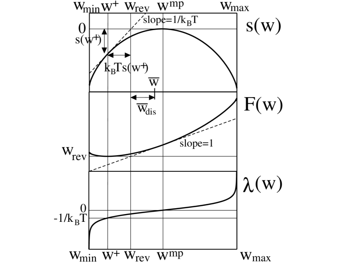
Figure 1: Diagrams showing the different relevant quantities in the trajectory thermodynamics formalism. Upper panel: Trajectory entropy $s(w)$ related by (20) to the density of trajectories with work equal to $w$. Middle panel: Trajectory free-energy ${\cal F}(w)=w-k_{B}Ts(w)$. Lower panel: Lagrange multiplier $\lambda(w)$. Six are the most relevant work values: $w_{\rm max}$ and $w_{\rm min}$ for the maximum and minimum values of the work; $w^{\rm mp}$ the most probable work value given by $s^{\prime}(w^{\rm mp})=\lambda(w^{\rm mp})=0$ or ${\cal F}^{\prime}(w^{\rm mp})=1$; $w^{{\dagger}}$ the value of the work that has to be sampled to recover free energies from non-equilibrium work values using the Jarzynski equality (26). This is given by $s^{\prime}(w^{{\dagger}})=-\lambda(w^{{\dagger}})=1/k_{B}T$ or ${\cal F}^{\prime}(w^{{\dagger}})=0$; $w_{\rm rev}=F(H_{f})-F(H_{i})$ the reversible work; and $\overline{w_{\rm dis}}=\int_{w_{\rm min}}^{w_{\rm max}}(w-w_{\rm rev})P_{N}(w)dw$ the average dissipated work. They are related by $w_{\rm min}<w^{{\dagger}}<w^{\rm mp}<w_{\rm max}$ while the second law of thermodynamics imposes $w_{\rm dis}\geq 0$.

The difference between $w^{{\dagger}}$ and $w^{\rm mp}$ indicates that the average (29) is properly weighed whenever trajectories with work values around $w^{{\dagger}}$ are sampled. This result indicates that proper sampling of non-equilibrium work values around $w^{{\dagger}}$ is required to derive equilibrium free-energies from non-equilibrium measurements by using the Jarzynski equality. A proper sampling of work values around $w^{{\dagger}}$ can be guaranteed when, out of the total number of trajectories, a finite fraction of work trajectory values in the vicinity of $w^{{\dagger}}$ is observed. From a practical point of view this means that the histogram of work values must extend down to $w^{{\dagger}}$. If this is not achieved, then the exponential average performed over a finite number of non-equilibrium experiments has a bias that can be estimated in some cases [14, 15]. Eqs.(31,32) are readily solved at the Gaussian level (i.e. assuming that $P_{N}(w)$ is exactly a Gaussian or $s(w)$ a quadratic function) giving $w^{{\dagger}}=w^{\rm mp}-\sigma_{w}^{2}/k_{B}T$ ($\sigma_{w}^{2}$ being the variance of the Gaussian work distribution). For quasi-reversible processes in the linear response regime [15], the fluctuation-dissipation theorem implies $\sigma_{w}^{2}\simeq 2k_{B}Tw^{\rm mp}_{\rm dis}$ giving $w^{{\dagger}}_{\rm dis}\simeq-w^{\rm mp}_{\rm dis}$, i.e. trajectories with negative values of the dissipated work that are of the order (in absolute value) of the average dissipated work must be sampled to quantitatively verify the validity of the Jarzynski equality. An example of such a quasi-reversible process, where $P_{N}(w_{\rm dis})$ is exactly a Gaussian, is the case of a Brownian particle subjected to an harmonic potential and dragged in a fluid [8, 16, 17].

4 Numerical solution of the equations

Equations (13,14,15) can be numerically solved in general. We assume Glauber transition rates given by

$$p^{\rm up}(H)=p^{\rm tot}(H)q(H)~{}~{}~{};~{}~{}~{}p^{\rm down}(H)=p^{\rm tot}(H)(1-q(H))$$ (35)

with $q(H)=(1+\tanh(\beta\mu H))/2$ and $p^{\rm tot}(H)=1/\tau_{\rm relax}(H)=\alpha(H)$ corresponding to the inverse of the relaxation time. In this case,

$$p^{\rm up}(s)=\alpha(H(s))\frac{\exp(\beta\mu H(s))}{2\cosh(\beta\mu H(s))}$$ (36)

$$p^{\rm down}(s)=\alpha(H(s))\frac{\exp(-\beta\mu H(s))}{2\cosh(\beta\mu H(s))}~{}~{}~{}~{}.$$ (37)

Inserting these expressions in (11,12) we obtain,

$$c(s)=-\alpha(H(s))\frac{\sinh(2\gamma(s)+\beta\mu H(s))}{\cosh(\beta\mu H(s))}+\alpha(H(s))\tanh(\beta\mu H(s))$$ (38)

$$d(s)=\alpha(H(s))\frac{\cosh(2\gamma(s)+\beta\mu H(s))}{\cosh(\beta\mu H(s))}-\alpha(H(s))~{}~{}~{}.$$ (39)

The solution of the equations consists of the following steps:

1. Solution of ${\bf\gamma_{\lambda}(s)}$. With the boundary condition at the final time $s=t$, $\gamma_{\lambda}(t)=0$, Eq. (15) has to be numerically integrated backwards in time. Inserting (36,37) in (15) we obtain,

   $$\dot{\gamma}(s)=\lambda\mu\dot{H}(s)+\alpha(H(s))\sinh(\gamma(s))\bigl{(}\cosh(\gamma(s))+\sinh(\gamma(s))\tanh(\beta\mu H(s))\bigr{)}~{}~{}~{}~{}.$$ (40)

   However, a direct numerical integration of this equation leads to divergences and numerical instabilities. It is then convenient to express (40) in terms of a new variable $\epsilon(s)=1/\cosh(\gamma(s))$ which displays smooth behavior. Equation (40) becomes,

   $$\dot{\epsilon}(s)=-\frac{\tanh(\gamma(s))}{\cosh(s)}\Bigl{(}\lambda\mu\dot{H}(s)+$$

   $$\alpha(H(s))\sinh(\gamma(s))\bigl{(}\frac{1}{\epsilon(s)}+\sinh(\gamma(s))\tanh(\beta\mu H(s))\bigr{)}\Bigr{)}$$ (41)

   with the boundary condition $\epsilon(t)=1$. This equation can then be easily numerically integrated to give $\gamma_{\lambda}(s)$ for a given value of $\lambda$.

2. Solution of ${\bf m_{\lambda}(s)}$. Once the solution of (41) for a given value of $\lambda$, $\gamma_{\lambda}(s)$, is found, then it is possible to integrate (14) to find $m_{\lambda}(s)$. Because (14) is linear its solution can be explicitly written,

   $$m_{\lambda}(s)=m_{\lambda}(0)\exp\bigl{(}\int_{0}^{s}A_{1}(u)du\bigr{)}+\int_{0}^{s}duA_{2}(u)\exp\bigl{(}\int_{u}^{s}A_{1}(v)dv\bigr{)}$$ (42)

   with the definitions,

   $$A_{1}(s)=\alpha(H(s))\frac{\sinh(2\gamma_{\lambda}(s)+\beta\mu H(s))}{\cosh(\beta\mu H(s))}$$ (43)

   $$A_{2}(s)=-\alpha(H(s))\frac{\cosh(2\gamma_{\lambda}(s)+\beta\mu H(s))}{\cosh(\beta\mu H(s))}$$ (44)

   with the initial condition $m_{\lambda}(0)=\tanh(\gamma_{\lambda}(0)+\beta\mu H_{i})$.

3. Evaluation of ${\bf w,s(w),{\cal F}(w)}$. Once $\gamma_{\lambda}(s),m_{\lambda}(s)$ are known then we can evaluate $w$ using (13), the entropy $s(w)$ using (21) and the free energy ${\cal F}(w)=w-k_{B}Ts(w)$.

4. Dependence of the numerical algorithm on the sign of ${\bf\lambda}$. We must emphasize that the solution of the equations previously described only works in a sector of values of $\lambda$ of a given sign, $\lambda<0$, and leads to numerical instabilities in the other sector, $\lambda>0$, indicative that the transformation $\epsilon(s)=1/\cosh(\gamma(s))$ is inappropriate for $\lambda>0$. We have found a simple way out to this problem. It can be easily proven that the solution of (15) for a given value of $\lambda>0$ is equivalent to the solution of that equation with the value of $\lambda$ with its sign reversed ($-\lambda<0$) and for the reversed field protocol $H_{r}(s)=-H(s)$ (the subindex $r$ stands for reversed). Eq. (15) can then be solved and the resulting reversed solutions $m_{r}(s),\gamma_{r}(s),c_{r}(s),d_{r}(s)$ give the final solutions for the original value of $\lambda>0$: $m(s)=-m_{r}(s),\gamma(s)=-\gamma_{r}(s),c(s)=-c_{r}(s),d(s)=d_{r}(s)$ (all change sign except $d(s)$). At first glance, this symmetry property might seem to be related to the content of the fluctuation theorem. However this relation is only apparent because the reversed process in this case does not correspond to the time-reversal protocol which should be instead $H_{r}(s)=H(t-s)$ (see the discussion below in Sec. 5).

For the present numerical analysis, and for the sake of simplicity, we will consider a particular example where the ramping field $H(s)$ changes from $H(0)=H_{i}$ to $H(t)=H_{f}$ at a constant rate $r=\dot{H}$,

$$H(s)=H_{i}+rs~{}~{}~{},~{}~{}~{}r=\dot{H}=\frac{H_{f}-H_{i}}{t}~{}~{}~{}.$$ (45)

We will also consider $p^{\rm tot}(H)=\alpha$ independent of the field. This tantamount to assume that $p^{\rm tot}(H)$ corresponds to a microscopic attempt frequency or, rather, that the activation barrier is field independent. We numerically solved the equations in natural units $\mu=k_{B}T=1$ and we have chosen $\alpha=1$ as the characteristic relaxation timescale of the system. Results for different values of $H_{i},H_{f}$ have been obtained by doing ramping experiments at different values of the ramping speed $r$. In Figure 2 we show, in the particular example $H_{i}=0,H_{f}=1$, the results for the magnetization trajectory solutions $m_{\lambda}(s)$ and the Lagrange multiplier $\gamma_{\lambda}(s)$. These are plotted as a function of the time-dependent field $H(s)$ for different values of $\lambda$ and for a given value of the ramping speed. In Figs. 3, 4 we show several trajectory thermodynamics quantities at different ramping speeds ($r=0.01,0.1,1,10$). In the left panel of Figure 3 we plot the magnetization for the most probable trajectories $m_{\lambda=0}(s)$ as a function of $H(s)$. In the right panel of Figure 3 and in Figure 4 we show the different trajectory thermodynamics quantities as a function of $w_{\rm dis}$: the inverse temperature $\lambda(w_{\rm dis})$, the trajectory entropy $s(w_{\rm dis})$ and the trajectory free-energy ${\cal F}(w_{\rm dis})$.

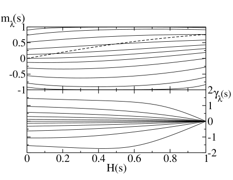
Figure 2: Protocol with $H_{i}=0,H_{f}=1$ and ramping speed $r=1$. Curves correspond to different values of $\lambda$ ($\lambda=-5,-2,-1,-0.5,-0.2,0.,0.2,0.5,1,2,5$ from top to bottom in the upper and lower panel). Upper panel: Magnetization $m_{\lambda}(s)$ obtained from (42). The dashed line is the equilibrium magnetization $m_{\rm eq}(H)=\tanh(H)$ corresponding to the reversible ramping experiment $r=0$. Lower panel: Lagrange multiplier $\gamma_{\lambda}(s)$ obtained from (41). Note the boundary condition $\gamma_{\lambda}(t)=0$ and the presence of the most probable trajectory $\gamma_{\lambda=0}(s)=0,\forall s$.

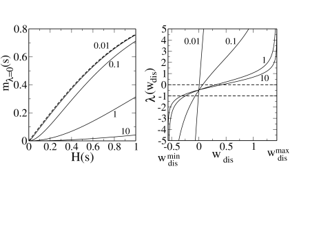
Figure 3: Protocol with $H_{i}=0,H_{f}=1$ and different ramping speeds $r=0.01,0.1,1,10$ (indicated by numbers along the continuous curves in both panels). The reversible work is $w_{\rm rev}=-0.433781$ and $w_{\rm max}=1,w_{\rm dis}^{\rm max}=w_{\rm max}-w_{\rm rev}=1.433781,w_{\rm dis}^{\rm min}=w_{\rm min}-w_{\rm rev}=-0.566219$. Left panel: magnetization evolution for the most probable trajectories. The dashed line corresponds to the reversible trajectory for $r\to 0$. Right panel: Lagrange multiplier $\lambda(w_{\rm dis})$ for different ramping speeds. The intersection of the different curves with the dashed line $\lambda=0$ gives $w^{\rm mp}$ while the intersection with $\lambda=-1$ gives $w^{{\dagger}}$. The intersection of all lines at different speeds around $\lambda=-0.5$ is only accidental (looking at a larger resolution or considering other parameters for the protocol such common crossing does not exist).

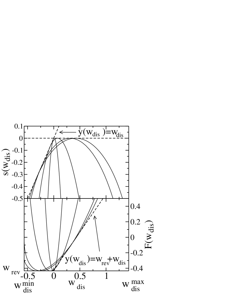
Figure 4: Same parameters and ramping speeds as in Figure 3. Narrower curves correspond to lower ramping speeds. Upper panel: Dynamical entropies $s(w)$ plotted as functions of $w_{\rm dis}=w-w_{\rm rev}$. According to the trajectory thermodynamics relations (31,32) the straight line $y(w_{\rm dis})=w_{\rm dis}/k_{B}T$ (we take $k_{B}T=1$) is tangent to the curve $s(w_{\rm dis})$ at $w_{\rm dis}=w_{\rm dis}^{{\dagger}}=w^{{\dagger}}-w_{\rm rev}$ and crosses the $w_{\rm dis}$-axis at $w_{\rm dis}=0,s(w_{\rm dis})=0$. All entropies vanish at $w_{\rm dis}=w_{\rm dis}^{\rm mp}=w^{\rm mp}-w_{\rm rev}$. Lower panel: Trajectory free-energy ${\cal F}(w_{\rm dis})$. It is identical to the equilibrium free-energy change $\Delta F=w_{\rm rev}$ at $w_{\rm dis}=w_{\rm dis}^{{\dagger}}$. According to the same relations (31,32) the straight line $y(w_{\rm dis})=w_{\rm rev}+w_{\rm dis}$ is tangent to the curve ${\cal F}(w_{\rm dis})$ at $w_{\rm dis}=w_{\rm dis}^{\rm mp}=w^{\rm mp}-w_{\rm rev}$ and crosses the $w_{\rm dis}$-axis at $w_{\rm dis}=0,{\cal F}(w_{\rm dis})=w_{\rm rev}$.

4.1 Average and variance of the work distribution

As has been schematically depicted in Figure 1 there are different work quantities that can be of relevance to characterize work fluctuations. We have already defined the most probable work $w^{\rm mp}$ and the work $w^{{\dagger}}$. Another important quantity is the average work $\overline{w}$,

$$\overline{w}=\int_{w_{\rm min}}^{w_{\rm max}}w\,P_{N}(w)\,dw$$ (46)

where $P_{N}(w)$ was defined in (4) or in approximate form in (20). In most cases (for instance, when the work distribution has asymmetric tails) the average work $\overline{w}$ is different from the most probable work $w^{\rm mp}$. $\overline{w}$ can be lower or higher than the most probable work $w^{\rm mp}$. However, in our large-$N$ theory, $w^{\rm mp}=\overline{w}$ and we will use indistinctly both quantities in this section. We defer the discussion about finite-size effects in these quantities until Sec. 7. Another important quantity that characterizes the work distribution is its variance,

$$\sigma_{w}^{2}=\overline{w^{2}}-(\overline{w})^{2}=\overline{w_{\rm dis}^{2}}-(\overline{w_{\rm dis}})^{2}~{}~{}~{}.$$ (47)

The average work $\overline{w}$ (or $w^{\rm mp}$) is the most relevant physical quantity that connects with classical thermodynamics. The second law of thermodynamics establishes that it cannot be lower than the reversible work, $\overline{w}\geq w_{\rm rev}$. However, it is clear that there can be WF such that $w<w_{\rm rev}$. These have been called transient violations (TV) of the second law. The relevant work value characterizing this sector of trajectories is given by $w^{{\dagger}}$. Clearly, $\overline{w}$ is always higher than $w^{{\dagger}}$. In Figure 5 (left panel) we show the dependence of $w_{\rm dis},w^{{\dagger}}$ with the ramping speed when the field is ramped from $H_{i}=0$ to $H_{f}$ for different values of $H_{f}$.

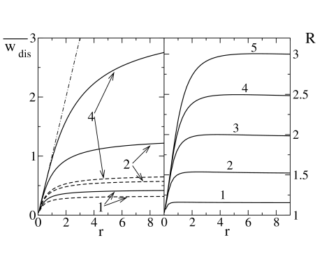
Figure 5: Ramping experiments with $H_{i}=0$ and different values of $H_{f}$ as function of the ramping speed $r$. Left panel: $w_{\rm dis}$ (continuous lines) and $-w^{{\dagger}}_{\rm dis}$ (dashed lines) for different values of $H_{f}$ indicated in the figure. The dash-dotted straight line corresponds to the linear response behavior $w_{\rm dis}=r$ given by (51). Note that $w^{{\dagger}}_{\rm dis}$ is negative so we changed its sign in order to compare it with $w_{\rm dis}$. Right panel: Fluctuation-dissipation ratio $R$ as a function of $r$ evaluated at different values of $H_{f}$ (from bottom to top, $H_{f}=1,2,3,4,5$).

It is possible to write down explicit analytic expressions for the cumulants of the distribution $P_{N}(w)$ in the large-$N$ limit. Interestingly, and due to the non-interacting character of the model (2), the cumulants derived from the large-$N$ approach are exact at all values of $N$, see Sec. 7. In particular, the first moment is given by,

$$\overline{w_{\rm dis}}=w^{\rm mp}-w_{\rm rev}=$$

$$2\mu\int_{0}^{t}ds\dot{H}(s)\int_{0}^{s}du\dot{H}(u)\frac{\partial q(H)}{\partial H}\Bigr{|}_{H=H(u)}\exp\Bigl{(}-\int_{u}^{s}dv\alpha(H(v))\Bigr{)}~{}~{}~{}.$$ (48)

The expression for the second cumulant or variance can be obtained by expanding the function $s(w)$ (21) up to second order with $\lambda(w)$ as the small parameter. Using the result $s^{\prime}(w^{\rm mp})=0$ we get

$$s(w)=s(w^{\rm mp})+\frac{1}{2}\Bigl{(}\frac{\partial^{2}s(w)}{\partial w^{2}}\Bigr{)}(w-w^{\rm mp})^{2}+{\cal O}\Bigl{[}(w-w^{\rm mp})^{3}\Bigr{]}~{}~{}~{}.$$ (49)

From (20) and (22) we obtain the relation,

$$\sigma_{w}^{2}=\frac{1}{N}\Bigl{[}\frac{\partial^{2}s(w)}{\partial w^{2}}\Bigr{|}_{w=w^{\rm mp}}\Bigr{]}^{-1}=\frac{1}{N}\frac{dw(\lambda)}{d\lambda}\Bigr{|}_{\lambda=0}$$ (50)

We do not reproduce the details of this lengthy calculation here, the same results have been already obtained in a slightly different context in a previous work and in the limit of large free-energy changes $\Delta F$ as compared to $k_{B}T$ [12].

Another interesting aspect of the present theory is that it is possible to expand the cumulants around the limits $r\to 0$ or $r\to\infty$. The former is particularly interesting because it corresponds to the so-called linear-response regime. In Reference [12] this regime was considered by expanding the average dissipated work up to linear order in the perturbation speed. By using dimensional arguments and direct comparison with the equivalent expression derived in the context of mechanical force [12] we can derive the following result,

$$\overline{w_{\rm dis}}=\frac{\mu\Delta M}{N\tau_{\rm relax}(H_{c}=0)}r+{\cal O}(r^{2})$$ (51)

where $\Delta M=M_{\rm eq}(H_{f})-M_{\rm eq}(H_{i})$ is the difference of equilibrium magnetizations between the initial and final values of the field whereas $\tau_{\rm relax}(H_{c}=0)=1/p_{\rm tot}(H_{c}=0)$ is the relaxation time at the critical value of the field where the configurations $\sigma=+1$ and $\sigma=-1$ are equiprobable (i.e. $H_{c}=0$). The linear response regime breaks down for large ramping speeds when $\overline{w_{\rm dis}}\ll w_{\rm rev}$. An interesting quantity quantifying deviations from the linear-response regime is the fluctuation-dissipation ratio $R$ defined by,

$$R=\frac{\sigma_{W}^{2}}{2k_{B}T\overline{W_{\rm dis}}}=\frac{\sigma_{w}^{2}}{2k_{B}T\overline{w_{\rm dis}}}~{}~{}~{}.$$ (52)

In the limit of small $r\to 0$, when $\overline{w_{\rm dis}}\propto r$, then $R$ converges to 1 (in agreement with the fluctuation-dissipation theorem, a result that in the context of steady-state systems has been proven in [13]) but deviates from 1 as $r$ increases. In the right panel of Figure 5 we show $R(r)$ when the field is ramped from $H_{i}=0$ to $H_{f}$ at different values of $H_{f}$. In this case the behavior of both $\overline{w_{\rm dis}}$ and $R$ is monotonic with $r$. In Figure 6 we show the same ramping experiments but comparing, for a given ramping speed, the results for $w_{\rm dis},-w^{{\dagger}},R$ as a function of $H_{f}$ . For values of $H_{f}$ small enough the ramping process is well described by the linear response-approximation discussed in Sec. 3 and $w^{{\dagger}}_{\rm dis}\simeq-w^{\rm mp}_{\rm dis}$.

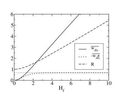
Figure 6: Ramping experiment with $H_{i}=0$ and $r=100$ as a function of $H_{f}$. The average dissipated work $w_{\rm dis}^{\rm mp}$ (continuous line) and $R$ (dashed line) increase with the field but $w_{\rm dis}^{{\dagger}}$ (dotted line) saturates to a finite value equal to $-\log(2)$ (we represent $-w_{\rm dis}^{{\dagger}}$ in order to compare with $w_{\rm dis}^{\rm mp}$).

Let us finish this section emphasizing that the dependence $R(r)$ can be quite complicated and even non-monotonic in some cases. Such behavior is observed in the case where the ramping protocol is given by $H(s)=H_{A}(1-2s/t)$, i.e. the field starts at a given value $H_{i}=-H_{A}$ ($H_{A}$ denotes the field amplitude) and increases until its reversed value $H_{f}=H_{A}$ is reached. This case is of much interest regarding heat fluctuations and is discussed in detail in Sec. 6. In Figure 7 we show the behavior of the average work $\overline{w}$ (equal to the average dissipated work as $w_{\rm rev}=0$ due to the independence of the free energy on the sign of $H_{A}$) and $R$ as a function of the ramping speed for different values of $H_{A}$.

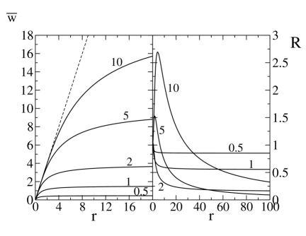
Figure 7: Average work $w$ (left) and fluctuation-dissipation ratio $R$ (right) for the case $H_{f}=-H_{i}=H_{A}$ as a function of the ramping speed. The different curves correspond to different values of the amplitude field $H_{A}$. These are indicated in the plot besides each curve. The straight dashed line in the left panel corresponds to the linear-response relation $\overline{w}=2r$ in (51). As explained in last paragraph of Sec. 5, and for this particular protocol, the relation $w^{{\dagger}}=-w^{\rm mp}$ is exact for all values of $r$ and $H_{A}$. Moreover, for large values of $H_{A}$ the work coincides with the heat exchanged, see Sec. 6.

5 The fluctuation theorem

Saddle-point equations (13,14,15) were derived in the large-$N$ limit. Indeed (20) is not exact for finite $N$ but has corrections. However, the results obtained for $s(w)$ exactly satisfy the fluctuation theorem of Crooks [5]. This theorem states the following: let us consider a process where the system is perturbed according to a protocol $H_{F}(s)$ during the time interval $[0,t]$, initially the system being in equilibrium at the value of the field $H_{i}=H_{F}(0)$. We will call this the forward (F) process. Let us now consider the reverse process defined as the time-reversed of the forward process: in this process the system starts in equilibrium at time $s=0$ at the value of the field $H_{i}=H_{F}(t)$ and the field is changed according to the protocol $H_{R}(s)=H_{F}(t-s)$. Let the distribution of works generated in this way be $P_{F}(W),P_{R}(W)$ for the forward (F) and reverse (R) processes respectively. The two distributions satisfy the following relation [5],

$$\frac{P_{F}(W)}{P_{R}(-W)}=\exp\Bigl{(}\frac{W-\Delta F}{k_{B}T}\Bigr{)}=\exp\Bigl{(}\frac{W_{\rm dis}}{k_{B}T}\Bigr{)}$$ (53)

where $\Delta F=F(H_{f})-F(H_{i})$ is the change in the equilibrium free-energy. By rewriting this identity as $P_{R}(-W)=P_{F}(W)\exp\Bigl{(}\frac{-W+\Delta F}{k_{B}T}\Bigr{)}$ and integrating it between $W=-\infty$ and $W=\infty$ leads to the Jarzynski equality $<\exp(-W_{\rm dis}/k_{B}T)>_{F}=1$ where $<...>_{F}$ stands for a dynamical average over work values obtained along the forward process.

If we now substitute (20) into the relation (53) we obtain,

$$s_{F}(w_{\rm dis})-s_{R}(-w_{\rm dis})=\frac{w_{\rm dis}}{k_{B}T}$$ (54)

where we have taken $P_{F,R}(W)\propto\exp(Ns_{F,R}(w))$ and we have disregarded the normalization constant in the distribution (20) as unimportant. Because the quantity $s(w)$ used in (20) is only exact in the large-$N$ limit one might be tempted to think that (54) does not hold. To prove the validity of (54) we rewrite (53) in the following way,

$$\frac{1}{N}\log(P_{F}(W))-\frac{1}{N}\log(P_{R}(-W))=\frac{W_{\rm dis}}{Nk_{B}T}~{}~{}~{}.$$ (55)

In the large-$N$ limit the distributions (20) satisfy,

$$\lim_{N\to\infty}\frac{1}{N}\log(P_{F,R}(W))=s_{F,R}(W)$$ (56)

and therefore (54) is exact with $w_{\rm rev}=\lim_{N\to\infty}\Delta F/N$. The present approach seems quite general so the trajectory entropy derived in a large-$N$ theory in any statistical model (interacting or non-interacting) must verify the relation (54). Another interesting relation that can be obtained from (54) relates the values of $w^{\rm mp},w^{{\dagger}}$ for the forward and reverse processes. Differentiating (54) respect to $w$ we obtain,

$$s^{\prime}_{F}(w)+s^{\prime}_{R}(-w)=\lambda_{R}(-w)-\lambda_{F}(w)=\frac{1}{k_{B}T}$$ (57)

where we used (22). Therefore, the identity $s^{\prime}_{F}(w^{\rm mp})=\lambda_{F}(w^{\rm mp})=0$ (23) implies $s^{\prime}_{R}(-w^{\rm mp})=\lambda_{R}(-w^{\rm mp})=1/k_{B}T$. From (31) we then infer that $w^{{\dagger}}$ for the reverse process is identical to $-w^{\rm mp}$ for the forward process and vice versa. This relation is quite interesting because it suggests that in order to estimate (e.g. in experiments) the value of $w^{{\dagger}}$ for a given non-equilibrium process it is enough to determine $w^{\rm mp}$ for the reversed process, a quantity that is experimentally accessible.

An interesting case of (53) occurs whenever the forward and reverse processes are symmetrical mirror images, $H_{F}(s)=-H_{R}(s)=-H_{F}(t-s)$. This can be accomplished when $H_{A}=H_{f}=-H_{i}$ along the forward process and the protocol satisfies $H(s)=-H(t-s)$. In this case the forward and the reverse work distributions are identical, $W_{\rm rev}=\Delta F=0$ (or $w=w_{\rm dis}$) and (54) reads,

$$s(w)-s(-w)=\frac{w}{k_{B}T}$$ (58)

where we have used $s(w)=s_{F}(w)=s_{R}(w)$. The validity of (58) can be further demonstrated by close inspection of equations (13,14,15). Let $s(w)$ be the value of the dynamical entropy for a given value of the work $w$ associated to the value of the Lagrange multiplier $\lambda$ and the magnetization $m(s)$. Then, for the reversed value of the work $-w$, it is possible to show that the corresponding solutions are: $-\lambda-1/k_{B}T$ for the Lagrange multiplier and $-m(t-s)$ for the magnetization solution. The resulting entropy is then $s(-w)=s(w)-w/k_{B}T$ as given in (58). A remarkable consequence of this special case is the aforementioned fact that $w^{{\dagger}}=-w^{\rm mp}$ at any ramping speed and for any value of ther amplitude of the field $H_{A}$. This case was already shown in Figure 7. The present symmetric case is specially interesting because the work done upon the system can be identified with the heat exchanged between the system and the bath. The conditions required for such identification are discussed next.

6 Heat fluctuations and tails

Until now we focused our efforts to investigate work fluctuations. However, in the same way as the work fluctuates, the heat exchanged between the system and the bath also does. The validity of the mechanical equivalence of heat (the content of the first law of thermodynamics) suggests that there should not be an important difference between heat and work. Heat is more difficult to experimentally measure than work and this is the reason why we tend to be more interested in the former.

A motivation to investigate heat fluctuations has recently arisen in the context of steady state and aging systems. In the first case, heat fluctuations were investigated for the simple model of a bead dragged through a viscous fluid [17]. In the second case these were studied for the case of a spin-glass model characterized by slow dynamics and aging [18, 19, 20]. In both cases, a Gaussian component was identified in the heat distributions together with some exponential tails. For the steady state system these exponential tails were consequence of the validity of an asymptotic fluctuation-theorem for the heat while in the aging system the tails were the signature of intermittency effects that have been experimentally observed in glasses and colloids [21, 22].

The heat along a given trajectory can be inferred using energy conservation, $-Q+W=\Delta E$. To extract the heat we just need to know the change in energy $\Delta E$ between the final and initial configurations as well as the work $W$. Here we adopt the sign convention (contrary to that adopted in the introduction Sec. 1) that positive heat corresponds to net heat delivered by the system on the surroundings. A particular case where work and heat fluctuations are identical is the case described in the preceding section where $H_{f}=-H_{i}=H_{A}$. Due to time reversal symmetry $W_{\rm rev}=\Delta F=0$. Now, if the field amplitude $H_{A}$ is large enough, the difference in energy $\Delta E=-\mu\Delta(MH)$ is practically zero so $Q=W$. For example, if $H_{A}=5$, then $\tanh(5)=0.99991$ (as always we take $\beta=\mu=1$) so the initial equilibrium magnetization is $M_{\rm eq}(H_{A})=-N$. The final magnetization after ramping the field to $H_{A}$ is again of order $N$ and therefore the fluctuations from trajectory to trajectory in $\Delta E$ are negligible as compared to the total work. In Figure 8 we show the trajectory entropy and free-energy for the case $H_{A}=10$. We have chosen to represent variables in terms of heat per particle $q=Q/N$ rather than work to give a view of what general shape we can expect from heat distributions. In terms of the heat we expect that the same mathematical definitions and relations that we defined in the case of work are also valid. For instance, the heat entropy and the heat free-energy are defined in the same way as we did for their work counterparts just replacing $w$ by $q$, in particular ${\cal F}(q)=q-k_{B}Ts(q)$. Also the equivalent of (22) holds,

$$\frac{\partial s(q)}{\partial q}=-\lambda(q)$$ (59)

The most probable heat $q^{\rm mp}$ ($\lambda(q^{\rm mp})=0$) and the quantity $q^{{\dagger}}$ ($\lambda(q^{\rm mp})=-1$) can also be defined. Moreover, a relation equivalent to (58) is also expected to hold for large enough values of $H_{A}$,

$$s(q)-s(-q)=\frac{q}{k_{B}T}~{}~{}~{}.$$ (60)

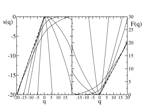
Figure 8: Trajectory entropy $s(q)$ and trajectory free-energy ${\cal F}(q)$ for the case $H_{f}=-H_{i}=10$ at ramping speeds $r=0.1,0.5,1,10,100$ (from the most narrower to the most wider distributions). The dashed line in the left panel is $y(q)=q/k_{B}T$ (we take $k_{B}T=1$) and is tangent to $s(q)$ at a value $q^{{\dagger}}$. The dashed line in the right panel corresponds to $y(q)=q$ and is tangent to ${\cal F}(q)$ at the value $q^{\rm mp}$. Both $q^{\rm mp},q^{{\dagger}}$ depend on the ramping speed.

An interesting aspect of the heat entropy $s(q)$ shown in the left panel of Figure 8 is the presence of quadratic behavior for small values of $q$ ($q\simeq 0$) together with a linear behavior in the tails ($|q|>>1$). These characteristic features of the heat entropy $s(q)$ can be inferred by looking at $\lambda(q)$, shown in Figure 9. That figure shows that $\lambda(q)$ is linear with $q$ for $q\simeq 0$, giving a quadratic behavior for $s(q)$ at small values of $q$. This linear shape in $\lambda(q)$ corresponds to a Gaussian distribution for $P(q)=\exp(s(q))$. It also shows that for a wide range of $|q|$ values there are two plateaus at $\lambda(q)\sim\lambda_{+},-\lambda_{-}$ for positive and negative values of $q$ respectively. These plateaus correspond to the exponential tails in the distribution.

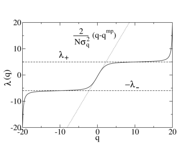
Figure 9: $\lambda(q)$ for the same parameters as in Figure 8 in the case $r=0.1$. We note the presence of a linear behavior for $\lambda(q)$ for small values of $q$, $\lambda(q)=(2/N\sigma_{q}^{2})(q-q^{\rm mp})$ ($q^{\rm mp}=0.207,N\sigma_{q}^{2}=0.83$) and two plateaus for $q>>1$ and $q<<-1$ ($\lambda_{+}=4.95,\lambda_{-}=5.95$). The former gives rise to the Gaussian component in the heat distribution describing the statistics of most probable values. The latter gives rise to two exponential tails for the distribution describing the statistics of rare events.

This behavior is quite generic at all ramping speeds, the distinction in $\lambda(q)$ between both plateaus and the linear behavior at small $q$ becomes more clear as the speed decreases. In such conditions, $q^{\rm mp}$ is not very large and the linear response approximation holds. The Gaussian sector describes the statistics of small and most probable fluctuations, the exponential tails describe rare events and large deviations. In what follows we analyze the Gaussian and exponential tails in more detail.

In the region where both $q,q^{\rm mp}$ are not too large we have,

$$s(q)=-\frac{1}{N\sigma_{q}^{2}}(q-q^{\rm mp})^{2}~{}~{}~{}~{}~{}~{}q,q^{\rm mp}<<1$$ (61)

Substituting this relation in (60) we get,

$$s(q)-s(-q)=\frac{2q^{\rm mp}}{N\sigma_{q}^{2}}q=\frac{q}{k_{B}T}$$ (62)

implying

$$\frac{N\sigma_{q}^{2}}{2q^{\rm mp}k_{B}T}=1$$ (63)

This result shows that the fluctuation-dissipation ratio (52) is equal to 1 if heat fluctuations are restricted to the sector of $q$ small. Small fluctuations are a key assumption of linear-response theory which also leads to (63).

This quadratic behavior then goes over straight lines in the most negative and positive sectors of $q$,

$$s(q)=C-\lambda_{+}q~{}~{}~{}~{}~{}q>>1$$ (64)

$$s(q)=C+\lambda_{-}q~{}~{}~{}~{}~{}q<<-1$$ (65)

where $C$ is a constant and $\lambda_{+},\lambda_{-}$ correspond to the values of $\lambda(q)$ in the plateaus shown in Figure 9. Note that the constant $C$ in (64,65) is the same in both sectors. In fact, the relation (60) imposes such constraint between the positive and negative tails in the probability distributions. Substituting (64,65) into (60) we obtain

$$\lambda_{-}-\lambda_{+}=\frac{1}{k_{B}T}$$ (66)

meaning that the width of the tails is larger for the negative values of $q$ than for positive values. This can be interpreted by saying that, despite of the fact that the average heat $q$ is positive, rare fluctuation events occur as often for $q<0$ (i.e. when the system adsorbs heat from the surroundings) as they do for $q>0$ (when the system delivers heat to the surroundings). The shape of the heat distribution $P(q)=\exp(s(q))$ is then dominated by a central Gaussian distribution with exponential tails at its extremes. These features are illustrated in Figure 10.

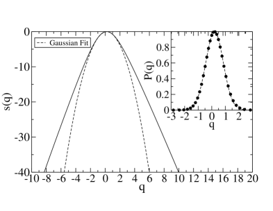
Figure 10: Heat entropy $s(q)$ for the case $H_{f}=-H_{i}=10$ at ramping speed $r=0.1$. Main figure: The sector of small or most probable fluctuations $q\sim 0$ can be well fitted to the Gaussian (61) (dashed line) with parameters $q^{\rm mp}=0.207,N\sigma_{q}^{2}=0.83$ satisfying (63). The tails extend beyond the Gaussian central part and are of exponential type as described in (64,65) with $\lambda_{-}=5.95,\lambda_{+}=4.95,C=9.16$. These exponential tails describe the statistics of large deviations or rare events. Inset: Heat-distribution $P(q)=\exp(s(q))$ (dots) and the Gaussian fit (the dashed line of the main figure) showing that the small $q$ sector of fluctuations (those that are frequently observable) is very well fitted by a Gaussian despite of the fact that rare-event tails are big and observable only when plotting $s(q)$ or the distribution $P(q)$ in logarithmic scale.

If the amplitude field $H_{A}$ is not large enough there may be contributions to the heat distribution coming out from the fluctuations in the difference in energy between the initial and final configurations. The effect of the value of $H_{A}$ on the value of the average work and the fluctuation-dissipation ratio have been already shown in Figure 7, in particular non-monotonic behavior is observed for $R$.

7 Finite-size effects

The method we developed in this paper allowed us to calculate $P_{N}(w)$ in the large-$N$ limit. However, due to the non-interacting character of the model, all cumulants of the distribution obtained in the large-$N$ limit are also exact for finite $N$. The proof is quite straightforward. Let us define the generation function of all cumulants of the distribution $P_{N}(W)$ in (4),

$$g_{N}(x)=\log\Bigl{(}\overline{\exp(xW)}\Bigr{)}=\log\Bigl{(}\int dW\exp(xW)P_{N}(W)\Bigr{)}~{}~{}~{}.$$ (67)

Cumulants of $P_{N}(W)$ are obtained using the following formula,

$$c_{N}(k)=\frac{\partial^{k}g_{N}(x)}{\partial x^{k}}\Bigr{|}_{x=0}~{}~{}~{},$$ (68)

$k$ being a positive integer. Using the non-interacting character of the model then we can write,

$$W=\sum_{i=1}^{N}w_{i}\rightarrow g_{N}(x)=Ng_{1}(x)\rightarrow c_{N}(k)=Nc_{1}(k)$$ (69)

and therefore all cumulants of the distribution are independent of the size of the system (except by a multiplicative constant equal to $N$). This implies that the expression given for $\overline{w_{\rm dis}}$ in (48) and $R$ in (52) are independent of $N$. Therefore, the results we obtained in the large-$N$ limit are exact for any finite value of $N$.

However, albeit cumulants do not depend on $N$, the shape of the distribution $P_{N}(w)$ in (20) depends on the size $N$ and only in the large-$N$ limit the approximate distribution (20) becomes exact. For instance, the value of $w^{\rm mp}$ depends on $N$ and converges to $\overline{w_{\rm dis}}$ for large enough values of $N$. In practice, already for $N=5-10$ convergence of the approximate distribution (20) to the exact result is excellent. In order to compare the approximate distributions we obtain from our theory with the exact ones at finite $N$ we have done numerical simulations of the model. The simulation procedure is described below in Sec. 8. In Figure 11 we show the distributions we have obtained for $N=10$ compared to the numerical simulations at different ramping speeds. The agreement between theory (continuous lines) and simulations (symbols) is good although it worsens progressively as the ramping speed increases and the system is strongly driven out of equilibrium. An important feature of the distributions is observed for large $r$ and small $N$: the presence of a finite fraction of trajectories that dissipate a maximum amount of work equal to $w_{\rm max}=\mu(H_{f}-H_{i})$. For these trajectories the ramping speed is so high and the size so small that no change in the initial configuration occurs along the trajectory. We will call these trapped trajectories. The fraction of trapped trajectories contributes with a term $\delta(w-w_{\rm max})$ to the work distribution,

$$P_{N}(w)=\tilde{P}_{N}(w)+\alpha(N)\delta(w-w_{\rm max})$$ (70)

where $\tilde{P}_{N}(w)$ is a continuous function and $\alpha(N)$ is a size-dependent constant that decreases with $N$ and asymptotically vanishes in the large-$N$ limit. The delta function in (70) is a small $N$ contribution that is not captured by the present large-$N$ theory. Nevertheless, it might be analytically derived using the approach described below in Sec. 7.1.

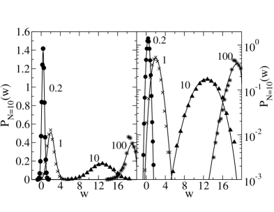
Figure 11: Distributions $P_{N}(w)$ for case $H_{f}=-H_{i}=10$ and $N=10$ at different ramping speeds (indicated along each curve). The continuous lines are the results obtained from the present theory using (20). The symbols are results obtained from numerical simulations of the model for $10^{4}$ trajectories. The right panel is the same figure but in logarithmic scale. For the largest ramping speed $r=100$ there is a finite fraction of trajectories (about $37\%$ of the total number of trajectories) where the spins have no time to relax. These trajectories contribute with a singular term at $w=w_{\rm max}=20$ to the distribution $P_{N=10}(w)$ as described in (70). It cannot be captured by the present large-$N$ theory so we did not include it in the histogram obtained from the numerical simulations.

In Figure 12 we show the effect of the size on the distributions at a moderate ramping speed. For $N=1$ the agreement is not good although the behavior of the left tails is reasonably well reproduced. However, already for $N=5$ the agreement has improved considerably. We conclude that it is between $N=1$ and $N=5$ that finite-size effects are important. In Figure 13 we confirm this strong small-$N$ dependence by plotting the most probable work as obtained from the numerical simulations as a function of $r$ for different sizes $N=1,2,5,20$.

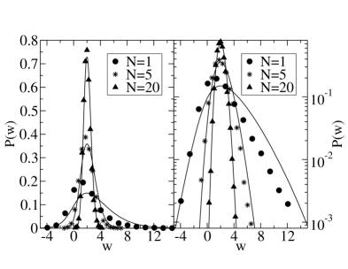
Figure 12: The same as in Figure 11 but showing the dependence of $P_{N}(w)$ with $N$ at $r=1$. The agreement is not good for $N=1$ in the central region of the distribution but is reasonably good for the left tail of the distribution (see the right plot in logarithmic scale). The agreement improves noticeably beyond $N\simeq 5$.

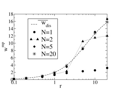
Figure 13: The same parameters as in Figure 11 but now showing the dependence of the most probable work value $w^{\rm mp}$ with $N$. The different symbols in the points correspond to different sizes as indicated in the legend of the figure. The continuous dashed line is $w^{\rm mp}$ as derived from the theory in the large-$N$ limit (where $w^{\rm mp}=\overline{w_{\rm dis}}$, the latter being independent of $N$). In the linear-response regime, $r<<1$, data have converged to the theory for all sizes. Although finite-size effects are large for $N=1,2$ and $r>>1$, already for $N=5$ the simulations have converged to the theory at all ramping speeds. Data for $N=2$ have been connected by a dotted line to emphasize the sharp increase of $w^{\rm mp}$ around $r\simeq 5$. This sharp increase originates from the presence of two separated peaks in the work distribution which height coincide at a given value of the ramping speed around $r\simeq 5$.

7.1 Reconstructing $P_{1}(w)$ from the large-$N$ theory

A crucial aspect of the present model is that it is non-interacting. Therefore, if we were to know the work probability distribution for $N=1$ (a single spin) then we could reconstruct the general distribution $P_{N}(w)$. In fact, let $\hat{P}_{N}(s)$ denote the Laplace transform of $P_{N}(w)$,

$$\hat{P}_{N}(s)=\int_{0}^{\infty}\exp(-Ws)P_{N}(W)dW$$ (71)

Using the result $W=\sum_{i=1}^{N}w_{i}$ we can write,

$$\hat{P}_{N}(s)=\bigl{(}\hat{P}_{1}(s)\bigr{)}^{N}$$ (72)

allowing us to reconstruct $P_{N}(w)$ from the sole knowledge of $P_{1}(w)$. Although the analytical computation of $P_{1}(w)$ might be possible by using other approaches, throughout this paper we have considered a thermodynamic approach where the large-$N$ theory has been taken as an approximation to finite $N$. This approach turns out to give exact results for all cumulants of the distribution thereby suggesting that the reconstruction of $P_{1}(w)$ from $P_{N}(w)$ might be possible. One could naively think that this is possible just using (72) together with the knowledge of $P_{N}(w)$. Unfortunately, this is not the case as the knowledge of $P_{N}(w)$ is only approximate as we showed in the previous section. There is however a possible strategy to reconstruct $P_{1}(w)$ that is based on the fact that cumulants are exactly known. Let us define the following function,

$$h(x)=\lim_{N\to\infty}\frac{g_{N}(x)}{N}$$ (73)

where $g_{N}(x)$ was defined in (67). In the large-$N$ limit we can solve $h(x)$ by applying the saddle-point approximation,

$$h(x)=\lim_{N\to\infty}\frac{1}{N}\log\Bigl{(}\overline{\exp(xW)}\Bigr{)}=$$

$$\lim_{N\to\infty}\frac{1}{N}\log\Bigl{(}\int dW\exp(xW)\exp(Ns(w))\Bigr{)}=xw(x)+s(w(x))~{}~{}~{}.$$ (74)

where $w(x)$ is the solution of the equation,

$$\frac{ds(w)}{dw}\Bigr{|}_{w=w(x)}=-x~{}~{}~{}.$$ (75)

For a given value of $w$, (22) shows that $x=\lambda(w)$. For instance, for $x=0,-1/k_{B}T$ we get $w=w^{\rm mp},w^{{\dagger}}$ respectively. Therefore, we can express $h(x)$ in terms of $w$ rather than $x$,

$$h(w)=w\lambda(w)+s(w)$$ (76)

By inserting (69) in (73) we get $g_{1}(w)=h(w)$ and therefore,

$$\int dw^{\prime}\exp\Bigl{(}\lambda(w)(w^{\prime}-w)\Bigr{)}P_{1}(w^{\prime})=\exp\Bigl{(}s(w)\Bigr{)}$$ (77)

Formally, this integral equation is closed and provides an exact solution for $P_{1}(w)$ in terms of the entropy $s(w)$. Unfortunately we have been unable to solve it in full generality (as detailed knowledge of the solution in (75) is required). Yet, for $P_{1}(w)$ it still holds that there are exponential tails identical to those we already derived for $P_{N}(w)$ in the large-$N$ limit. To show this result we use (22) and rewrite (77) as follows,

$$\int dw^{\prime}\exp\Bigl{(}-s(w)-\frac{\partial s(w)}{\partial w}(w^{\prime}-w)\Bigr{)}P_{1}(w^{\prime})=1~{}~{}~{}.$$ (78)

Let us now suppose now that $\lambda(\omega)$ is approximately constant (equal to $\hat{\lambda}$) showing a plateau over a given region of work values. From (22) then $s(w^{\prime})\simeq s(w)+\frac{\partial s(w)}{\partial w}(w^{\prime}-w)$ and,

$$P_{1}(w^{\prime})\propto\exp(s(w^{\prime}))=C\exp(\hat{\lambda}w^{\prime})~{}~{}~{},$$ (79)

where $C$ is a constant. This shows that the width of the exponential tail for $P_{1}(w)$ (and, by extension, for $P_{N}(w)$ at any value of $N$) is equal to $\hat{\lambda}$.

8 The case of magnetic nanoparticles

In this section we discuss a system where the previous theory could be experimentally tested. We focus our attention on thermally activated magnetic nanoparticle systems [23]. These systems have the great advantage that dynamics is invariant under time-reversal of the magnetic field $H\to-H$. Also many magnetic field cycles can be experimentally realized in micro-SQUID machines allowing to experimentally extract the work distribution with good precision. The main experimental limitation to observe WF though is the quite large value of the magnetic moment of the nanoparticle. Transition rates are described by the Brown-Neel formula,

$$\tau_{\rm relax}(H)=\tau_{0}\exp\Bigl{(}\frac{B(H)}{k_{B}T}\Bigr{)}$$ (80)

where $\tau_{0}$ is a microscopic time describing relaxation within a state and $B(H)$ is a field dependent barrier. We consider two cases: A) paramagnetic molecular clusters where the energy barrier is nearly field independent $B(H)=B_{0}$ (this case could also describe specific ferro and ferrimagnetic nanoparticles where the anisotropy contribution to the zero-field barrier is negligible, for a discussion see [24]); B) ferromagnetic nanoparticles with axial anisotropy where $B(H)$ depends on the intensity of the external field projected on the easy magnetization axis as described by the Stoner-Wohlfarth expression $B(H)=B_{0}(1-\Bigl{|}\frac{H}{H_{c}}\Bigr{|})^{\alpha}$ where $H_{c}$ is the field required to suppress the barrier and $\alpha$ is an exponent in the range $1.5-2$. Recent experiments have demonstrated how the height of the barrier $B_{0}$ can be considerably reduced by applying a transverse field, making possible to observe magnetization reversible transitions (also called telegraph noise measurements) in single Co nanoparticles at low temperatures [25, 26].

As we already discussed in Sec. 5, in a magnetic system a time-reversal invariant protocol can be accomplished by switching the magnetic field $H$ from $-H_{A}$ to $H_{A}$ ($H_{A}$ being the amplitude of the field), the free energy and the rates being an even function of $H$. Under such conditions work and heat are equivalent if $H_{A}$ induces a magnetization close to its saturation value. From the experimental point of view, it is relevant to understand under which conditions large deviations from the most probable work are observable. By large deviations we understand work (heat) fluctuations corresponding to work (heat) values around $w^{{\dagger}}$ ($q^{{\dagger}}$). A useful quantity that tell us how difficult it is to sample that region of work values is the ratio $\Omega$ describing the fraction of trajectories that transiently violate the second law, $w\leq 0$. This fraction is given by the integrated fluctuation theorem [2, 5]. This is obtained by rewriting (53),

$$P_{N}(-W)=P_{N}(W)\exp\Bigl{(}-\frac{W-\Delta F}{k_{B}T}\Bigr{)}=\exp\Bigl{(}-\frac{W_{\rm dis}}{k_{B}T}\Bigr{)}~{}~{}~{}~{}.$$ (81)

where we have taken $P_{N}(W)=P_{F}(W)=P_{R}(W)$. Integrating this expression from $W=0$ up to $W=\infty$ we obtain,

$$\Omega=\frac{{\cal N}(w<0)}{{\cal N}(w>0)}=\langle\exp(-\frac{Nw}{k_{B}T})\rangle_{w>0}$$ (82)

where ${\cal N}(w<0),{\cal N}(w>0)$ are the fraction of trajectories for which the total work is negative and positive respectively,

$${\cal N}(w<0)=\int_{-\infty}^{0}dWP(W)~{}~{}~{}~{};~{}~{}~{}~{}{\cal N}(w>0)=\int_{0}^{\infty}dWP(W)$$ (83)

and the average on the r.h.s of (82) is restricted to the subset of trajectories for which $w>0$. Quite generally, we expect that $\Omega$ is a non-universal function dependent on all cumulants of $s(w)$, yet its exponential dependence in $N$ assures that, in the regime where TV are observable, $\Omega$ is approximately described by the value of the average total work divided by the bath temperature $\overline{W}/k_{B}T$ which is approximately given by $Nw^{\rm mp}/k_{B}T$.

We choose Glauber rates as these have been experimentally demonstrated to describe very well the relaxation of single magnetic moments [27, 28]. These are given by (35) where $\tau_{\rm relax}(H)$ is given by (80). We consider ramping experiments [29] where $N$ particles are subject to the action of a field that is switched from $H=-H_{A}$ up to $H=H_{A}$ at a constant speed $\dot{H}$. We generate individual trajectories according to the Glauber rates by starting from initial configurations with $M=M_{\rm eq}(H_{A})$ and repeating the ramping protocol many times, each time the total work (3) is computed, $W=-\mu\int_{-H_{A}}^{H_{A}}M(H)dH$. If $H_{\rm sw}$ is the field at which the magnetization of a given particle switches for the first time then, for a given trajectory, some of the particles will switch state at a value of the field $H_{\rm sw}<0$, while others will switch at $H_{\rm sw}>0$. For fast ramping speeds the dynamics is well described by a first-order Markov process [30] and the dissipated work for that trajectory will be identical to the value $2H_{\rm sw}$ averaged over all particles. In general, for lower ramping speeds, the relation between the dissipated work and the value of $H_{\rm sw}$ is more complicated. To estimate $\Omega$ we generate trajectories and evaluate the fraction of them with $W>0$ and $W<0$. We chose to do numerical simulations rather than applying the large-$N$ theory to give a more clear picture about which results can we expect from a finite number of ramping experiments (around 10000). In the main panel of Figure 14 we plot the value of $\Omega$ (82) as obtained for different ramping protocols in cases A and B. All points scatter around a generic (but non-universal) curve useful to predict in which regime TV are expected to be observable. An important advantage of the time-reversal symmetry property $H\to-H$ of magnetic nanoparticle systems, as compared to other systems [7, 8], is the feasibility of performing many ramping cycles in a single experiment making TV observable for $\Omega$ values as low as $10^{-4}$. According to Figure 14, TV should be observable for work values as large as $20k_{B}T$.

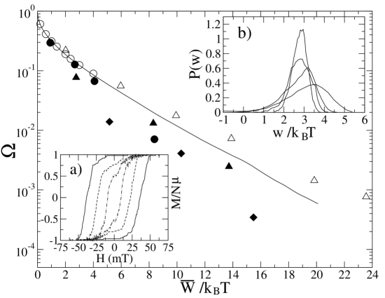
Figure 14: Application of the theory to magnetic nanoparticles for a case where $w_{\rm rev}=0$ and $w\simeq q$. Main panel: $\Omega$ (82) as a function of $\overline{W}/k_{B}T$ for Cases A and B. Number of particles range from $N=1$ up to $20$ for both cases. Case A) corresponds to nanoparticles (open symbols) with $\mu=300\mu_{B},T=200K,H_{A}=2{\rm T},\tau_{0}=10^{-7}s,B_{0}=2300K$ at ramping speeds $r=1{\rm mT}/s({\rm circles}),10{\rm mT}/s({\rm triangles\,up})$. Case B) corresponds to ferromagnetic particles (filled symbols) with $\mu=500\mu_{B},T=40K,H_{A}=238{\rm mT},H_{c}=119{\rm mT},B_{0}=500K,\tau_{0}=10^{-5}s,\alpha=1.5$ and ramping speeds of $0.01({\rm circles}),0.1({\rm triangles\,up}),1({\rm diamonds}){\rm T}/s$ (continuous,dashed and dotted lines respectively). The continuous line is the prediction for a Gaussian work distribution (see discussion at the end of Sec. 3) in the linear-response regime $\sigma_{w}^{2}=2k_{B}T\overline{w_{\rm dis}}$ ($R=1$ in (52)). Insets: Both are for ferromagnetic nanoparticles (Case B) with the same parameters as in the main panel. Inset a) shows hysteresis cycles for $N=100$ ferromagnetic nanoparticles at the three ramping speeds (larger hysteresis for higher speeds). Inset b) shows dissipated work distributions at ramping speeds $0.1{\rm T}/s$ for $N=1,5,10,20$ particles (larger sizes correspond to narrower distributions).

9 Conclusions.

Two-state systems provide a simple conceptual framework to analyze work fluctuations (WF) and transient violations (TV) of the second law. These non-equilibrium effects are expected to be relevant and observable for nanosized objects when the energies involved are several times $k_{B}T$, $k_{B}$ being the Boltzmann constant and $T$ the temperature of the bath. These have been already observed in the unfolding of small RNA hairpins [7] as well as in polysterene beads dragged through a solvent [8]. Related measurements include the experimental test of the Gallavotti-Cohen fluctuation theorem in Rayleigh-Bernard convection [9] and turbulent flows [10]. Other experiments include the observation of gravitatory potential energy fluctuations in driven granular media [31]. The scientific discipline behind all such rich phenomenology deserves to be called thermodynamics of small systems. It deals with the thermal behavior of non-equilibrium small systems where the typical energies are few times $k_{B}T$. The statistics of energy exchange processes between the system and the thermal environment is described by frequent Gaussian distributed events plus rare events corresponding to large statistical deviations from the average value. The theoretical and experimental study of these fluctuations could be of relevance to understand issues related to the organization and function of biological matter in the nanoscale [32].

In this paper we studied WF in two-state systems. We have introduced a trajectory thermodynamics formalism with the specific aim to quantify WF in such model. We have shown how to define a trajectory entropy $s(w)$ that characterizes WF around the most probable value $w^{\rm mp}$, and a trajectory free-energy ${\cal F}(w)$ whose minimum value at $w=w^{{\dagger}}$ specifies the value of the work that needs to be efficiently sampled to quantitatively test the Jarzynski equality. The theory requires the introduction of a Lagrange multiplier $\lambda(w)$, its inverse playing the role of a temperature in the trajectory thermodynamics formalism. Analytical expressions for the trajectory potentials $s(w),{\cal F}(w)$ have been also derived. In general, both values $w^{\rm mp}$ and $w^{{\dagger}}$ are of the same magnitude but opposite sign, meaning that large deviations of WF need to be sampled to recover equilibrium free-energies from non-equilibrium measurements, e.g. by using the Jarzynski equality.

We have then carried out a systematic study of WF in the framework of the large-$N$ theory. Several results are worth mentioning. First of all, we have found an analytical expression for the trajectory entropy that satisfies the fluctuation theorem by Crooks [5] that relates forward and reverse processes. An important result is that the value of the work $w^{{\dagger}}$ that has to be sampled in order to test the Jarzynski equality is equal to the most probable value of the work (with a minus sign) for the reverse process. Intuitively this means that the forward and reverse distributions must overlap each other in order to get good estimates of the work using the Jarzynski equality, a result that was emphasized long-time ago by Bennett [33]. Furthermore, if both forward and reverse processes are symmetric mirror images then $w^{\rm rev}=0$ and $w^{{\dagger}}=-w^{\rm mp}$ independently of how far the system is driven out of equilibrium . This last case is particularly interesting as the total work practically coincides with the heat. The fluctuation theorem by Crooks is then also applicable to the heat in that limit, a result that is quite reminiscent of a heat fluctuation theorem recently derived [17, 34]. For the heat distribution, we find that it is described by a central Gaussian distribution describing local equilibrium, i.e. with $R=1$, and long exponential tails with widths described by the Lagrange multiplier $\lambda(w)$, which plays the role of the inverse of a temperature. Strictly speaking, because the temperature must be a positive quantity, only the tails in the negative sector $q<<-1$ where $\lambda$ is negative admit such an interpretation (i.e. in the sector of WF dominated by TV). It has not escaped our attention that this temperature could be related to other non-equilibrium temperatures that have been defined in other contexts  [35, 36], such as steady-state [37] or aging systems [18].

Our study raises the following question: to what extent are work and heat fluctuations equivalent? We already emphasized in Sec. 6 that work and heat should be equivalent, at least this is the underlying content of the first law of thermodynamics. However, from the perspective provided by the present analysis, some important differences can be underlined. Exponential tails are more often observed in the heat rather than in the work. Such result has been explicitly shown in the case of a bead dragged through a fluid [17] where the work is clearly Gaussian distributed while the heat displays exponential tails. However, in that case the origin of this difference lies on the fact that the motion for the bead is described by a stochastic linear equation which in general might not be the case. The difference between heat and work has its root at the true microscopic definition of these quantities. Heat is identical to work when the final energy of the system is constrained be identical to the initial value (i.e. $Q=W$ if $\Delta E=0$, for the heat we adopt the sign convention of Sec. 6). The simplest interpretation is that exponential tails in the work distribution are always present if the model is non-linear by definition (which is not the case for the aforementioned case of the bead dragged through the fluid). However, work distributions always tend to be masked by a Gaussian contribution coming out from the Gaussian fluctuations that characterize the initial equilibrium state. Therefore, only when thermal fluctuations in the initial and final states are negligible as compared to the total amount of work along the trajectory, the measured work distributions are paralleled by the heat distributions and tails can be observed. This explains the qualitative difference observed between the functions $\lambda(w)$ in Figs. 9 and the right panel in Fig. 3. In the latter, Gaussian fluctuations in the energy of the initial and final configurations tend to mask the presence of the exponential tails.

We also studied finite-size effects to test how good the large-$N$ theory is and provided a strategy to re-derive the finite-$N$ work distribution from the large-$N$ result. An important conclusion is that the large-$N$ theory accounts for the existence of exponential tails also at finite $N$, the value of the widths $\lambda_{+},\lambda_{-}$ (corresponding to the plateaus in $\lambda(w)$) being independent of $N$. In addition, we applied the theory to magnetic nanoparticle systems which provide an experimental realization of two-state systems. We studied under which conditions the theory can be experimentally tested. Our results suggest that WF and TV should be observable whenever average work values are not much larger than $20k_{B}T$. It is realistic to say that we are currently at the limit of the resolution of current micro-SQUID devices for the detection of single small magnetic moments (around few hundreds of $\mu_{B}$). Surely, we will see developments in the near future and experimental measurements of WF in magnetic systems, as well as the test of the present theory, will become possible.

Acknowledgments. The author acknowledges the warm hospitality of Bustamante and Tinoco labs at UC Berkeley where this work was done. He is grateful to C. Bustamante, J. Gore, C. Jarzynski, A. Labarta and I. N. Tinoco for useful discussions. This work has been supported by the David and Lucile Packard Foundation, the Spanish Ministerio de Ciencia y Tecnología Grant BFM2001-3525 and Generalitat de Catalunya.

References

- [1] Evans, D., J., Cohen, E., G., D., & Morriss, G., P. (1993) Phys. Rev. Lett. 71, 2401-2404
- [2] Subsequent work has been reviewed in Evans, D. & Searles, D. (2002) Adv. Phys. 51, 1529
- [3] Jarzynski, C. (1997) Phys. Rev. Lett. 78, 2690
- [4] Kurchan, J. (1998) J. Phys. A (Math. Gen.) 31, 3719
- [5] Crooks, G. E. (1998) J. Stat. Phys. 90, 1481; (2000) Phys. Rev. E 61, 2361
- [6] Hummer, G., & Szabo, A. (2001) Proc. Natl. Acad. Sci. USA 98 3658-3661
- [7] Liphardt, J., Dumont, S., Smith, S., B., Tinoco, I., Jr., & Bustamante, C. (2002) Science 296, 1832-1835
- [8] Wang, G., M., Sevick, E., M., Mittag, E., Searles, D., J., & Evans, D. , J. (2002) Phys. Rev. Lett. 89, 050601
- [9] Ciliberto, S. & Laroche, C. (1998) J. Phys. IV (France) 8 215
- [10] Ciliberto, S., Garnier, N., Hernandez, S., Lacpatia C., Pinton J.-F. & Ruiz Chavarria G. (2003) Preprint arXiv:nlin.CD/0311037v2
- [11] Laughlin, R., B., Pines, D., Schmalian, J., Stojkovic, B., P., & Wolynes, P. (2000) Proc. Nat. Acad. Sci. USA 97, 32
- [12] Ritort, F., Bustamante, C., & Tinoco, I., Jr. (2002) Proc. Nat. Acad. Sci. USA 99, 13544
- [13] Gallavotti, G., Cohen, E., G., D., (1995) J. Stat. Phys. 80, 931
- [14] Zuckerman, D., M., & Woolf, T., B. (2002) Chem. Phys. Lett. 351, 445; (2002) Phys. Rev. Lett. 89, 180602
- [15] Gore, J., Ritort, F., & Bustamante, C. (2003) Proc. Nat. Acad. Sci. USA 100, 12564
- [16] Mazonka. O. & Jarzynski, C. (1999) Preprint arXiv:cond-mat/9912121
- [17] Van Zon, R., & Cohen, E., G., D. (2003) Phys. Rev. Lett. 91, 110601 ; (2003) Phys. Rev. E 67, 046102
- [18] Crisanti, A. & Ritort, F. (2004) Europhys. Lett. 66, 253
- [19] Ritort, F. Preprint arXiv:cond-mat/0311370 Proceedings of the workshop “Unifying concepts in granular media and glasses”. Eds. A. Coniglio, A. Fierro, H. J. Hermann and M. Nicodemi, Elsevier-Amsterdam (2004).
- [20] Ritort, F. (2004) J. Phys. Chem. B 108, 6893
- [21] Buisson, L., Bellon, L., & Ciliberto, S. (2003) J. Phys. C (Cond. Matt.) 15, S1163
- [22] L. Cipelletti et al., J. Phys. C (Cond. Matt.) 15, S257 (2003)
- [23] Wernsdorfer, W. (2001) Adv. Chem. Phys. 118, 99
- [24] Gonzalez-Miranda, J., M., & Tejada, J. (1994) Phys. Rev. B 49, 3867
- [25] Wernsdorfer, W., Bonet-Orozco, E., Hasselbach, K., Benoit, A., Barbara, B., Demoncy, N., Loiseau, A., Pascard, H. & Mailly, D. (1997) Phys. Rev. Lett. 78, 1791
- [26] Jamet, M., Wernsdorfer, W., Thirion, C., Dupuis, V., Mélinon, P., & Pérez, A. (2001) Phys. Rev. Lett. 86, 4676
- [27] Caneschi, A. et al. (2001) Preprint arXiv:cond-mat/0106224
- [28] Coulon, C. et al. (2004) Preprint arXiv:cond-mat/0404620
- [29] Kurkïjarvi, J. (1972) Phys. Rev. B 6, 832; Gunther, L., & Barbara, B. (1994) Phys. Rev. B 49, 3926; Garg, A. (1995) Phys. Rev. B 51, 15592
- [30] Hanggi, P., Talkner, P., & Borkovec, M. (1990) Rev. Mod. Phys. 62, 251
- [31] Feitosa, K. & Menon, N. (2004) Phys. Rev. Lett. 92, 164301
- [32] Ritort, F. (2003) Seminaire Poincaré, 2, 63; Preprint arXiv:cond-mat/0401311
- [33] Bennett, C., H., (1976) J. Comp. Phys. 22, 245
- [34] Van Zon, R., Ciliberto, S., Cohen, E., G., D. (2003) Preprint arXiv: cond-mat/0311629
- [35] For a review, Casas-Vazquez, J., & Jou, D. (2003) Rep. Prog. Phys. 66, 1937
- [36] For a review, Crisanti, A. & Ritort, F. (2003) J. Phys. A (Math. Gen.) 36, R181
- [37] Zamponi, F., Ruocco, G., & Angelani, L. (2004) Preprint arXiv: cond-mat/0403579