Shot Noise of a Tunnel Junction Displacement Detector

Abstract

We study quantum-mechanically the frequency-dependent current noise of a tunnel-junction coupled to a nanomechanical oscillator. The cases of both DC and AC voltage bias are considered, as are the effects of intrinsic oscillator damping. The dynamics of the oscillator can lead to large signatures in the shot noise, even if the oscillator-tunnel junction coupling is too weak to yield an appreciable signature in the average current. Moreover, the modification of the shot noise by the oscillator cannot be fully explained by a simple classical picture of a fluctuating conductance.

Spurred primarily by experiments in solid-state qubit systems, there has recently been considerable interest in understanding the noise properties of mesoscopic systems used as detectors QPCPapers ; MakhlinRMP ; KorotkovSN ; Pilgram ; Me ; Averin . Many new results have emerged, including an understanding of the connection between noise, back-action dephasing and information Pilgram ; Me ; Averin , and of the influence of coherent qubit oscillations on the output noise of a detector KorotkovSN . Not surprisingly, similar concerns arise in the study of nanomechanical oscillators. Recent experiments using single-electron transistors (SETs) have demonstrated displacement detection of such oscillators with a precision close to the maximum allowed by quantum mechanics Cleland ; Schwab . Given the interest in these systems, it is important to gain a better understanding of how a mesoscopic detector influences the behaviour of an oscillator, and vice-versa. Several works have addressed various aspects of this problem. In particular, it has been shown that an out-of-equilibrium detector can serve as an effective environment for the oscillator, providing both a damping coefficient and an effective temperature MozTJ ; Moz ; Blencowe .

In the present work, we turn our attention to the finite-frequency output noise of a mesoscopic displacement detector, where one expects to see signatures of the time-dependent fluctuations of the oscillator. A completely classical study of the current noise of a DC-biased SET displacement detector was presented recently in Refs. ArmourSI, and BlanterSHO, . In contrast, we consider a generic tunnel-junction or quantum point-contact (QPC) detector, in which the tunnelling strength depends on the position of the oscillator, and calculate quantum mechanically the finite frequency current noise. Such a system could be realized by using an STM setup where one electrode is free to vibrate Yurke ; Konrad . We treat both DC and AC voltage bias; the latter is of particular interest, as in experiment, it is common to imbed the detector in a resonant tank circuit for impedance-matching purposes, and then probe its AC response. We find that even for a detector-oscillator coupling so weak that there is little signature of the oscillator in the average current, there can nonetheless be a strong signature in the finite-frequency current noise. We moreover find that the oscillator contribution to the noise cannot be simply explained by a classical model of a detector conductance which fluctuates with the oscillator position– there are additional quantum corrections which suppress the contribution of zero point fluctuations. We show that these quantum corrections result from correlations between the detector’s random back-action force and intrinsic noise. Finally, in the AC-biased case, we find that the oscillator experiences a time-dependent temperature, which has a direct influence on the detector’s current noise.

Model- Considering the simplest case where the tunnel-matrix element depends linearly on the oscillator displacement $\hat{x}$, the tunnel junction detector is described by:

$$H_{det} = \frac{\tau_{0}+e^{i\eta}\tau^{\prime}\hat{x}}{2\pi\Lambda}\sum_{k,k^{\prime}}\left(Y^{{\dagger}}c^{{\dagger}}_{R,k}c^{\phantom{\dagger}}_{L,k^{\prime}}+{\textrm{h}.c.}\right)-eV(t)\hat{m}$$

$$\equiv H_{det,0}-\hat{x}\cdot\hat{F}$$

Here, $c_{L,k}$ ($c_{R,k}$) destroys an electron state in the left (right) electrode, $\Lambda$ is the conduction-electron density of states, $\hat{m}$ denotes the number of tunnelled electrons, and the operator $Y^{\dagger}$ augments $\hat{m}$ by one. $\eta$ parameterizes the sensitivity of the transmission phase to $\hat{x}$, and will in general be non-zero etaNote . We consider both the cases of a pure DC voltage, $V(t)=\tilde{V}$ and a pure AC voltage, $V(t)=\tilde{V}\cos\nu t$. Note that the tunnelling Hamiltonian itself acts as a random back-action force $\hat{F}$ on the oscillator; this corresponds to random momentum shifts imparted to the oscillator by tunnelling electrons Yurke . We will describe our system by a reduced density matrix $\rho(m;x,x^{\prime};t)\equiv\langle x|\hat{\rho}(m;t)|x^{\prime}\rangle$ which tracks the state of the oscillator and $m$, the number of electrons which have tunnelled through the junction. As there is no superconductivity, $\hat{\rho}$ is diagonal in $m$. In general, the evolution of $\hat{\rho}$ will be given by a Dyson-type equation:

$$\frac{d}{dt}\hat{\rho}(m,t) = -\frac{i}{\hbar}\left[H_{0},\hat{\rho}(m;t)\right]+\int_{t_{0}}^{t}dt^{\prime}\sum_{m^{\prime}}$$

$$\check{\Sigma}(m,m^{\prime};t-t^{\prime})\circ\left[U_{0}^{\phantom{\dagger}}(t-t^{\prime})\hat{\rho}(m^{\prime};t^{\prime})U_{0}^{{\dagger}}(t-t^{\prime})\right]$$

Here, $U_{0}$ is the evolution operator corresponding to the unperturbed (zero-tunnelling) Hamiltonian, and we have written the self-energy $\Sigma$ as a super-operator (i.e.  an operator acting on the space of density matrices).

We will consider the simplest case of weak tunnelling, and keep only self-energy terms which are lowest order in the tunnelling. $\Sigma$ is only non-vanishing if $m^{\prime}=m$ or $m^{\prime}=m\pm 1$; these two types of contributions correspond to “scattering out” and “scattering in” terms in a kinetic equation, and are given by the diagrams shown in Fig. 1. These diagrams correspond to standard tunnelling bubbles Schoeller , the only difference being that the tunnelling vertices can contain an $\hat{x}$ operator. If $\hat{x}$ appears at the $t^{\prime}$ end of a graph for $\Sigma(t,t^{\prime})$, $\hat{x}$ will evolve during the duration of the tunnelling event. As a result, the self energy $\check{\Sigma}$ has terms involving $\hat{p}$, and the final form of $\Sigma$ we obtain does not correspond to the oscillator-free case with $\hat{x}$ dependent rates. We also include perturbatively the effects of a high-temperature Ohmic heat bath ($k_{B}T_{bath}\gg\hbar\Omega$, with $\Omega$ being the oscillator frequency) on the oscillator using a Caldeira-Leggett description CL and the lowest-order Born diagrams in the self-energy (i.e.  same diagrams as in Fig. 1, with tunnelling bubbles replaced by environmental boson lines).

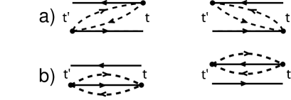
Figure 1: Diagrams for the a) scattering in, and b) scattering out terms in the self energy $\check{\Sigma}(t-t^{\prime})$. The solid lines represent the forward and backwards Keldysh contours; the dashed lines are conduction electron propagators. The solid black vertices correspond to $\tau_{0}+\tau^{\prime}\hat{x}$. Note that an $\hat{x}$ operator appearing in a vertex at time $t^{\prime}$ will evolve during the tunnelling event.

Finally, we specialize to the case where the voltage $\tilde{V}$ is much larger than $\hbar\Omega/e$. For weak tunnelling, $e\tilde{V}\gg\hbar\Omega$, and small AC frequency $\nu$, it is then possible to make a Markov approximation in Eq. (Shot Noise of a Tunnel Junction Displacement Detector): $U_{0}^{\phantom{\dagger}}(t-t^{\prime})\hat{\rho}(m^{\prime};t^{\prime})U_{0}^{{\dagger}}(t-t^{\prime})\rightarrow\hat{\rho}(m^{\prime};t)$. We are assuming that over the short timescales relevant to tunnelling, one can describe the dynamics of the density matrix by its zero-tunnelling evolution. Fourier-transforming in the $m$ index, $\hat{\rho}(k;t)=\sum_{m=-\infty}^{\infty}e^{ikm}\hat{\rho}(m;t)$, Eq. (Shot Noise of a Tunnel Junction Displacement Detector) becomes:

$$\frac{d}{dt}\hat{\rho}(k;t) = -\frac{i}{\hbar}\left[H_{0}-\bar{F}(t,\eta)\hat{x},\hat{\rho}\right]-i\left(\frac{\gamma_{0}+\gamma}{\hbar}\right)[\hat{x},\{\hat{p},\hat{\rho}\}]-\left(\frac{D_{0}+D(t)}{\hbar^{2}}\right)[\hat{x},[\hat{x},\hat{\rho}]]+\sum_{\sigma=+,-}\left(\frac{e^{i\sigma k}-1}{(\tau^{\prime})^{2}}\right)\times$$

$$\Bigg{(}\frac{2D_{\sigma}(t)}{\hbar^{2}}(\tau_{0}+e^{i\sigma\eta}\tau^{\prime}\hat{x})\hat{\rho}(\tau_{0}+e^{-i\sigma\eta}\tau^{\prime}\hat{x})+i\frac{\gamma_{\sigma}(t)}{\hbar}\left(\tau_{0}\tau^{\prime}\left(e^{i\sigma\eta}\hat{p}\hat{\rho}-e^{-i\sigma\eta}\hat{\rho}\hat{p}\right)+(\tau^{\prime})^{2}\left(\hat{p}\hat{\rho}\hat{x}-\hat{x}\hat{\rho}\hat{p}\right)\right)\Bigg{)}$$

where $\gamma_{0}$ is the intrinsic damping coefficient associated with the equilibrium bath, $D_{0}=2M\gamma k_{B}T_{bath}$ is the corresponding diffusion constant, and $\sigma=+(-)$ labels contributions from forward (backwards) tunnelling. The detector-dependent diffusion constant $D(t)=\sum_{\sigma}D_{\sigma}(t)$ and damping coefficient $\gamma(t)=\sum_{\sigma}\gamma_{\sigma}(t)$ are given by:

$$\gamma_{\sigma}(t) = \frac{\hbar}{2M\Omega}\left(\frac{\tau^{\prime}}{\tau_{0}}\right)^{2}\left(\frac{\Gamma_{\sigma}(t,\hbar\Omega)-\Gamma_{\sigma}(t,-\hbar\Omega)}{2}\right)$$ (3)

$$D_{\sigma}(t) = \frac{\hbar^{2}}{4}\left(\frac{\tau^{\prime}}{\tau_{0}}\right)^{2}\left(\Gamma_{\sigma}(t,\hbar\Omega)+\Gamma_{\sigma}(t,-\hbar\Omega)\right)$$ (4)

while $\bar{F}(t,\eta)=\sin\eta\left(\frac{\tau^{\prime}}{\tau_{0}}\right)\sum_{\sigma}2\sigma D_{\sigma}(t)/\hbar$ is the average back-action force exerted on the oscillator. $\Gamma_{\pm}(t,E)$ are the $\tau^{\prime}=0$ finite temperature forward and backwards inelastic tunnelling rates involving an absorbed energy $E$; these rates are time-independent in the case of a DC voltage. Note that we have neglected self-energy terms which renormalize the oscillator Hamiltonian; these are unimportant in the weak-tunnelling limit we consider.

Eq. (Shot Noise of a Tunnel Junction Displacement Detector) yields a compact description of the coupled detector-oscillator system; it is a generalization of an equation first derived (via an alternate approach) by Mozyrsky et al. MozTJ to an arbitrary detector in the tunnelling regime, including the possibility of an $x$-dependent tunnelling phaseetaNote , a nonlinear junction I-V, a time-dependent bias voltage, and intrinsic oscillator damping. Taking $k=0$ yields the equation for the reduced-density matrix of the oscillator, and (c.f.  Ref. MozTJ, ) has the Caldeira-Leggett form for a forced, damped oscillator in the high-temperature regime CL . In what follows, we focus for simplicity on the case of $T=0$ in the tunnel junction, and on $\eta=0$, which ensures $\bar{F}=0$ etaNote ; a non-zero $\bar{F}$ does not significantly change our results.

Shot Noise- Eq. (Shot Noise of a Tunnel Junction Displacement Detector) can in principle be used to calculate the full counting statistics of tunnelled charge as a function of time. By focusing solely on the time-dependence of the reduced second moment $\langle\langle m^{2}(t)\rangle\rangle$ (i.e.  variance), it is possible to calculate the symmetrized frequency-dependent current noise using the MacDonald formula MacDonald . In the case of an AC bias voltage, the noise will be a function of two times. We focus on the part of the noise that is independent of the average time co-ordinate, a quantity which is directly accessible in experiment. It is given by a modified version of the MacDonald formula:

$$S_{I}(\omega)=2e^{2}\omega\int_{0}^{\infty}dt\sin\omega t\int_{0}^{2\pi}\frac{d\phi}{2\pi}\cdot\partial_{t}\langle\langle m^{2}(t,\phi)\rangle\rangle$$ (5)

where $\phi$ is the initial phase of the AC voltage.

DC Bias- For a DC biased normal-metal junction at $T=0$, the tunnelling rates are given by $h\Gamma_{\sigma}(t,E)=(\tau_{0})^{2}(\sigma e\tilde{V}+E)\Theta(\sigma e\tilde{V}+E)$. Eqs. (3)-(4) yield $\gamma=\hbar\tau^{\prime 2}/(4\pi M)$ and $k_{B}T_{eff}=eV/2$ MozTJ . We find from Eqs. (Shot Noise of a Tunnel Junction Displacement Detector) and (5) that the current noise may be written as $S_{I}(\omega)=2e\langle I\rangle+\Delta S_{I}$, where the first term corresponds to purely Poissonian statistics, and the second term is a correction arising from correlations between the motion of the oscillator and the number of tunnelled electrons:

$$\Delta S_{I}(\omega) = \frac{4e^{3}\tilde{V}}{h}\omega\int_{0}^{\infty}dt\sin\omega t\hskip 3.0pt$$

$$\Big{(}\left(2\tau_{0}\tau^{\prime}\right)\langle\langle\hat{x}(t)\cdot m(t)\rangle\rangle+\left(\tau^{\prime}\right)^{2}\langle\langle\hat{x}^{2}(t)\cdot m(t)\rangle\rangle\Big{)}$$

Physically, the covariances appearing above arise from the $x$-dependence of the tunnelling probability– if $m(t)$ is larger than average, then it is likely that $x(t)$ and $x^{2}(t)$ are also larger than average. These covariances can be calculated directly from Eq. (Shot Noise of a Tunnel Junction Displacement Detector), and obey simple classical equations corresponding to a forced, damped harmonic oscillator. Consider first the contribution from $\langle\langle x\cdot m\rangle\rangle$ in Eq. (Shot Noise of a Tunnel Junction Displacement Detector), which is leading order in $\tau^{\prime}$. In calculating this covariance, one finds that the tunnel junction provides an effective driving force; we find a contribution:

$$\Delta S_{I}(\omega)\Big{|}_{1}=\frac{e^{3}\tilde{V}}{h}\left(2\tau_{0}\tau^{\prime}\right)^{2}\left(\frac{e\tilde{V}}{h}-\frac{\Omega}{4\pi}\frac{(\Delta x_{0})^{2}}{\langle x^{2}\rangle}\right)S_{x}(\omega)$$ (7)

where $S_{x}(\omega)=8\gamma\Omega^{2}\langle x^{2}\rangle/((\omega^{2}-\Omega^{2})^{2}+4\gamma^{2}\omega^{2})^{-1}$ is the spectral density of oscillator $x$ fluctuations obtained from Eq. (Shot Noise of a Tunnel Junction Displacement Detector), and $(\Delta x_{0})^{2}=\hbar/(2M\Omega)$ is the zero-point uncertainty in the oscillator position. The first term in Eq. (7) is exactly the answer expected (to lowest order in $\tau^{\prime}$) from a simple picture of a classically fluctuating junction conductance (i.e.  $\Delta S_{I}(\omega)=\tilde{V}^{2}S_{G}(\omega)$, where $S_{G}(\omega)$ is the spectral density of conductance fluctuations, and is in turn determined by $S_{x}(\omega)$). Equivalently, if we think of our junction as an $x$-to-$I$ amplifier having a gain $\lambda=2e\tilde{V}\tau_{0}\tau^{\prime}/h$, this first term corresponds to simply amplifying up the fluctuations of the oscillator: $\Delta S_{I}=\lambda^{2}S_{x}$. Eq. (7) yields a peak in $S_{I}(\omega)$ at $\omega=\Omega$; keeping only the leading term in $\tilde{V}$, the ratio of the peak-height to the background Poissonian noise (i.e.  the S/N ratio) is:

$$\frac{\Delta S_{I}(\omega=\Omega)}{2e\langle I\rangle}=4\tau_{0}^{2}\left(\frac{e\tilde{V}}{h\gamma_{tot}}\right)\frac{\alpha^{2}}{1+\alpha^{2}}\leq 4\left(\frac{\tau_{0}}{\tau^{\prime}}\right)^{2}\frac{2Me\tilde{V}}{\hbar^{2}}$$ (8)

where $\alpha^{2}=\tau^{\prime 2}\langle x^{2}\rangle/\tau_{0}^{2}$, $\gamma_{tot}=\gamma_{0}+\gamma$. Note that if $\alpha$ is small, there will be no sizeable signature of the oscillator in the average current (i.e.  $\delta\langle I\rangle/\langle I\rangle_{0}\simeq\alpha^{2}$), but there may nonetheless be a large peak in the noise if $e\tilde{V}/(h\gamma_{tot})$ is large. The upper bound in Eq. (8) corresponds to the optimal scenario, where there is no intrinsic (detector-independent) damping, and $\alpha\gg 1$. The maximum $S/N$ is determined by $eV$ and the sensitivity $\tau^{\prime}/\tau_{0}$, and can be arbitrarily large. Due to the dependence on $\gamma$, we find the surprising result that the maximum $S/N$ is inversely proportional to the detector sensitivity $\tau^{\prime}/\tau_{0}$. Note the marked difference from experiments attempting to detect coherent qubit oscillations in the detector current noise KorotkovSN , where back-action effects limit the $S/N$ to a maximum of $4$.

We turn now to the second term in Eq. (7), which is a lower-order in $\tilde{V}$ quantum correction to the classical result. It would appear to cause $\Delta S_{I}|_{1}$ to vanish in the limit $e\tilde{V}\rightarrow\hbar\Omega/2$, $\langle x^{2}\rangle\rightarrow(\Delta x_{0})^{2}$, i.e.  it suppresses a zero-point contribution to $\Delta S_{I}|_{1}$. (Of course, we cannot rigorously take this limit, as Eq. (Shot Noise of a Tunnel Junction Displacement Detector) is strictly only valid for $e\tilde{V}\gg\hbar\Omega$). A similar result was found for the average current $\langle I\rangle$ in Ref. MozTJ, , where a similar offset term could be traced to the inherent asymmetry between events in which energy is absorbed from the oscillator, versus those in which it is emitted to the oscillator. In the present case, the quantum correction to the noise in Eq. (7) can be given a classical interpretation– it arises from correlations between the intrinsic shot noise of the detector, and the back-action force $\hat{F}$ acting on the oscillator. If there are such correlations, we would expect classically the current noise to have the form:

$$\Delta S_{I}(\omega)=\lambda^{2}S_{x}(\omega)+2\lambda\textrm{Re }\left[g(-\omega)S_{IF}(\omega)\right]$$ (9)

where $S_{IF}(\omega)$ is the symmetrized cross-correlator between the junction current and back-action force noise, and $g(\omega)$ is the oscillator response function. Note that the second term above is $\propto\tilde{V}$, while the first is $\propto\tilde{V}^{2}$. It is well known that inversion symmetry forces $\textrm{Re }S_{IF}$ to vanish; this is what allows a QPC detector to reach the quantum limit for measuring a qubit Me ; Averin . However, at finite $\omega$, $\textrm{Im }S_{IF}$ is non-zero. Consequently, the second term above is non-zero; a direct perturbative calculation (assuming a thermal state for the oscillator) shows that this term corresponds to the second term in Eq. (7). Thus, we see that quantum corrections to the noise, which suppress zero-point contributions, can be associated with classical out-of-phase correlations between the random back-action force and the intrinsic detector output noise.

Finally, we return to Eq. (Shot Noise of a Tunnel Junction Displacement Detector) and examine the contribution from $\langle\langle x^{2}\cdot m\rangle\rangle$, a term which is higher-order in $\tau^{\prime}$. One finds:

$$\left[\Delta S_{I}(\omega)\right]_{2} = \frac{e^{3}\tilde{V}}{h}(\tau^{\prime})^{4}\left(\frac{e\tilde{V}}{h}-\frac{\Omega}{2\pi}\frac{(\Delta x_{0})^{2}}{\langle x^{2}\rangle}\right)$$ (10)

$$\times\int\frac{d\omega^{\prime}}{2\pi}S_{x}(\omega^{\prime})S_{x}(\omega-\omega^{\prime})$$

Again, the first term above agrees with the expectation for a classically fluctuating junction conductance; it yields peaks in $S_{I}$ at $\omega=0$ and $\omega=2\Omega$. The second term is a quantum correction, completely analogous to that found for $\Delta S_{I}|_{1}$.

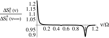
Figure 2: Oscillator contribution to $S_{I}^{a}$, the frequency-independent part of the shot noise (i.e.  second term in Eq. (13)), versus the AC voltage frequency $\nu$, for $\Omega/\gamma=50,\gamma_{0}=0$, and $e\tilde{V}\gg\hbar\nu,\hbar\Omega$. The maximum suppression of this term at $\nu=\Omega$ (over its $\nu\rightarrow\infty$ limit) is by 8/9.

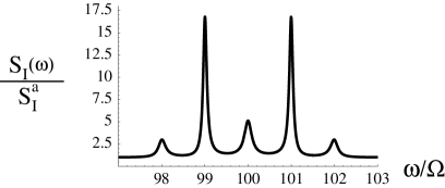
Figure 3: Full shot noise $S_{I}(\omega)$ for an AC bias voltage of frequency $\nu=100\Omega$, including the effects of correlations between $x(t)$ and $m(t)$ (c.f Eq. (14)). We have chosen $e\tilde{V}=100\hbar\Omega$, $\alpha^{2}=1$, $(\gamma_{0}+\gamma)=\Omega/20$, and $\tau_{0}=0.1$. The y-axis is scaled by the value of the $\omega$-independent part of the noise.

AC Bias- We now consider an AC bias voltage $V(t)=\tilde{V}\cos(\nu t)$, where $e\tilde{V}\gg\hbar\nu,\hbar\Omega$. In the limit of small $\nu$, it is possible to derive a simple expression for the time-dependent tunnelling rates Tucker . Defining $h\tilde{\Gamma}(E)=(\tau_{0})^{2}E\cdot\Theta(E)$, we have $\Gamma_{\sigma}(t,E)=\sum_{n=0}^{\infty}\left(1-\delta_{n,0}/2\right)\sigma^{n}\Gamma^{(n)}_{\sigma}(E)\cos n\nu t$, with:

$$\Gamma_{\sigma}^{(n)} = \sum_{\pm}\int_{0}^{\pi}\frac{d\theta}{\pi}\cos(n\theta)\tilde{\Gamma}\left(e\tilde{V}\cos\theta+E\pm\frac{n\hbar\nu}{2}\right)$$ (11)

Using Eqs. (3)-(4), we find that the damping coefficient $\gamma$ of the oscillator is time-independent and identical to that in the DC case, whereas the diffusion constant is time-dependent and contains higher harmonics of the AC frequency $\nu$. Writing $D(t)=2M\gamma k_{B}T_{eff}(t)$, we have to a good approximation:

$$k_{B}T_{eff}(t) = \frac{e\tilde{V}}{\pi}\left(\sum_{n=0}^{e\tilde{V}/\hbar\nu}\left(\frac{2(-1)^{n}}{1-(2n)^{2}}\right)\cos(2n\nu t)-1\right)$$

The small but finite photon frequency $\nu$ prevents higher harmonics from contributing to $T_{eff}$; without it, we would have simply $k_{B}T_{eff}(t)=\tilde{V}|\cos\nu t|/2$, which tends to zero twice each period. With the finite cut-off included, the minima of $k_{B}T_{eff}(t)$ are $\simeq\hbar\nu$. The time-dependence of $T_{eff}(t)$ implies that the position variance $\langle x^{2}(t)\rangle$ of the oscillator will be time-dependent and in phase with the AC voltage; as we show, this has a direct influence on the noise and the average current. For the latter quantity, we find:

$$\langle I(t)\rangle = \frac{e^{2}\tilde{V}}{h}\cos(\nu t)\left(\tau_{0}^{2}+(\tau^{\prime})^{2}\langle x^{2}(t)\rangle\right)-\Delta I(t)$$

where the quantum correction is approximately $\Delta I(t)\simeq e\gamma\cdot{\rm sgn}\left[\cos\nu t\right]$. Turning to the noise, we may again decompose $S_{I}(\omega)$ into a frequency-independent part and a term arising from correlations between $x(t)$ and $m(t)$: $S_{I}(\omega)\equiv\frac{\Omega}{2\pi}\int_{0}^{\frac{2\pi}{\Omega}}d\bar{t}S_{I}(\bar{t},\omega)=S_{I}^{a}+\Delta S_{I}(\omega)$. For the frequency-independent contribution $S_{I}^{a}$, we find:

$$S_{I}^{a}=\frac{4e^{2}}{h}\Bigg{[}\frac{e\tilde{V}}{\pi}\tau_{0}^{2}+(\tau^{\prime})^{2}\left(\overline{k_{B}T_{eff}(t)\langle x^{2}(t)\rangle}-\frac{\Omega}{2\pi}(\Delta x_{0})^{2}\right)\Bigg{]}$$ (13)

where the bar indicates a time-average. The first term is the standard result for the shot noise of an AC-biased junction PATNoise . The second term indicates that the time-dependent motion of $\langle x^{2}(t)\rangle$ (calculated from Eq. (Shot Noise of a Tunnel Junction Displacement Detector)) can make a frequency-independent contribution to the noise. For $\nu\gg\Omega$, $\langle x^{2}\rangle$ responds only weakly to the time-dependence of $T_{eff}(t)$, whereas for $\nu\sim\Omega$, the response becomes appreciable and $180$ degrees out-of-phase with $V(t)$. If in addition $\gamma_{0}\ll\gamma$, one finds a resulting suppression of the oscillator’s contribution to $S_{I}^{a}$; this is shown in Fig. 2. Small resonances also occur when $\Omega$ is a multiple of $\nu$. Note that the oscillator modification of $S_{I}^{a}$ is not captured by the classical picture of a fluctuating conductance.

Finally, the frequency-dependent contribution $\Delta S_{I}(\omega)$ to the noise, which arises from correlations between $x(t)$ and $m(t)$, takes the simple form:

$$\Delta S_{I}(\omega)=\frac{1}{4}\sum_{\pm}\Delta S_{I}(\nu\pm\omega)\Big{|}_{DC}\left[1+O\left(\frac{\hbar\Omega}{e\tilde{V}}\right)\right]$$ (14)

where the omitted terms correspond to “quantum corrections” of the sort previously discussed. Without these terms, Eq. (14) is precisely the answer expected for a fluctuating classical conductance– one needs to simply shift the noise in the DC case up to the frequency $\nu$. In contrast, the quantum corrections to $\Delta S_{I}$ for AC bias are not simply given by shifting the corresponding terms found for DC bias– one finds that the quantum corrections are larger in the AC case by a factor of $4/\pi$. The effect of $\Delta S_{I}(\omega)$ on the full noise is shown in Fig. 3.

In conclusion, we have presented a fully quantum mechanical calculation of the frequency-dependent current noise of a tunnel junction displacement detector, for both the cases of DC and AC voltage bias. The oscillator can lead to large effects in the shot noise, even if the coupling to the detector is weak; moreover, these effects cannot be completely described using a classical picture of a fluctuating junction conductance. We thank Konrad Lehnert and Florian Marquardt for useful discussions; this work was supported by the NSF under grant NSF-ITR 0325580, and by the W. M. Keck Foundation.

References

• (1) S. A. Gurvitz, Phys. Rev. B 56, 15215 (1997); I. L. Aleiner, N. S. Wingreen, and Y. Meir, Phys. Rev. Lett. 79, 3740 (1997); Y. Levinson, Europhys. Lett. 39, 299 (1997)
• (2) Y. Makhlin et al., Rev. Mod. Phys. 73, 357 (2001).
• (3) A. N. Korotkov and D. V. Averin, Phys. Rev. B 64, 165310 (2001)
• (4) S. Pilgram and M. BΓΌttiker, Phys. Rev. Lett. 89, 200401 (2002).
• (5) A. A. Clerk, S. M. Girvin and A. D. Stone, Phys. Rev. B 67, 165324 (2003).
• (6) D. V. Averin, cond-mat/0301524 (2003).
• (7) R. G. Knobel and A. N. Cleland, Nature 424, 291 (2003).
• (8) M. LaHaye et al., Science 304, 74 (2004).
• (9) B. Yurke and G. P. Kochanski, Phys. Rev. B 41, 8184 (1990).
• (10) K. Lehnert, private communication.
• (11) D. Mozyrsky and I. Martin, Phys. Rev. Lett 89, 018301 (2002).
• (12) D. Mozyrsky, I. Martin and M. B. Hastings, Phys. Rev. Lett 92, 018303 (2004).
• (13) A. D. Armour, M. P. Blencowe, and Y. Zhang, Phys. Rev. B 69, 125313 (2004)
• (14) A. D. Armour, cond-mat/0401387
• (15) Ya. M. Blanter, O. Usmani and Yu. V. Nazarov, cond-mat/0404615.
• (16) For example, in a tunnelling setup where the oscillator modulates the width of a rectangular barrier by moving the position of the right electrode (c.f. Ref. Yurke, ), one finds $\tan^{2}\eta=E_{F}/W$, where $W$ is the barrier height and $E_{F}$ the Fermi energy.
• (17) H. Schoeller and G. SchΓΆn, Phys. Rev B 50, 18436.
• (18) A. O. Caldeira and A. J. Leggett, Ann. Phys. (N.Y.) 149, 374 (1983).
• (19) D. K. C. MacDonald, Rep. Prog. Phys. 12, 56 (1948).
• (20) J. R. Tucker and M. J. Feldman, Rev. Mod. Phys. 57, 1055 (1985).
• (21) M. H. Pedersen and M. BΓΌttiker, Phys. Rev. B 58 (1998) 12993.