Amphiphiles at Interfaces: Simulation of Structure and Phase Behavior

Abstract

Computer simulations of coarse-grained molecular models for amphiphilic systems can provide insight into the the structure of amphiphiles at interfaces. They can help to identify the factors that determine the phase behavior, and they can bridge between atomic descriptions and phenomenological field theories.

Here we focus on model systems for amphiphilic membranes. After a brief general introduction, we present selected simulation results on monolayers, bilayers, and bilayer stacks. First, we discuss internal phase transitions in membranes and show that idealized models reproduce the generic phase behavior. Then we consider membrane fluctuations and membrane defects. The simulation data is compared with mesoscopic theories, and effective phenomenological parameters can be extracted.

1 Introduction

Amphiphilic molecules are characterized by the feature that they contain both water loving (hydrophilic) and water “hating” (hydrophobic) structural units. Familiar examples are alcohols or lipids (see Fig. 1). Amphiphiles are important for many applications in technology and nature. They are very effective at helping to dissolve different substances in water, which makes them very useful, e. g., as detergents, or as coating materials to stabilize colloidal systems. Furthermore, they form a rich variety of structures at higher concentrations. In order to shield their hydrophobic parts from the water, the amphiphiles self-assemble into spherical or cylindrical micelles or bilayers [1] (Fig. 2). These structures may then order on an even higher level and form superstructures (Fig. 3) [2, 3].

Figure 1: Structure of a single amphiphilic molecule (DPPC).

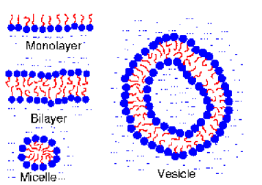
Figure 2: Self-assembled structures of amphiphiles in water.

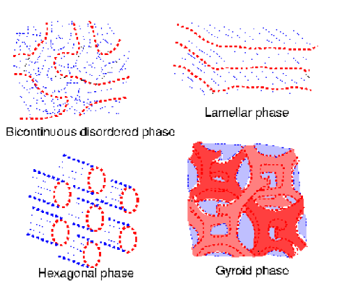
Figure 3: Selected structured phases in amphiphilic systems. The dashed lines represent bilayers. The different shadings in (d) distinguish between two different interwoven networks in the gyroid phase.

Particular interesting from an application point of view are those phases where the material is filled with bilayers. Such bilayer interfaces can serve as barriers against the diffusion of particles, and help to divide the space into compartments. Indeed, lipid bilayers are the structural basis of all biological membranes, which in turn play a central role for the function of all cells and cell organelles [4].

From an experimental point of view, studying the properties of biomembranes on a molecular scale in situ is not an easy task. Therefore, several model membrane systems have been developed: (i) monolayers at the air-water interface (Langmuir monolayers), (ii) stacks of bilayers, (iii) single planar bilayers, and (iii) giant vesicles. The simplest and oldest approach is to spread lipid molecules on a water surface [5]. Due to the amphiphilic nature of lipids, they form oriented monolayers at air/water interfaces. These are traditionnally placed in a Langmuir trough with a movable barrier on one side, which allows to control the surface area (see Fig. 4). The monolayers are then studied in the microscope, with $X$-ray scattering under conditions of grazing incidence, or simply by measuring the pressure-area isotherms. Since bilayers consist of two weakly coupled monolayers, many important bilayer properties can be studied already in monolayer systems.

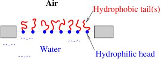
Figure 4: Schematic picture of a langmuir trough.

Another experimental approach to studying lipid bilayer membranes has been to examine lamellar stacks of bilayers, i. e., lamellar phases of lipids [6, 7, 8]. Highly aligned stacks have been prepared experimentally and then examined by $X$-ray diffraction [7, 8]. Such systems have also been useful to study the interactions of lipid membranes with other molecules, e. g., lipid-polymer interactions [9], lipid-protein interactions [10, 11], lipid-DNA interactions [12, 13].

Furthermore, there also exist techniques by which planar bilayers or giant bilayer vesicles can be generated. $X$-ray studies of such systems are difficult, due to the small size of the sample. However, they can be studied by other techniques, such as phase contrast microscopy or electron microscopy, light scattering, or transport measurements [4, 14]. It should be noted that isolated membranes are not stable in a thermodynamical sense. They are metastable structures, bound to break eventually. This, however, does not restrict their importance as model systems for biological membranes, which are themselves nonequilibrium structures.

When attempting to describe lipid membranes theoretically, one faces a problem that is common for soft materials: The membrane properties result from an interplay between physical and chemical phenomena that live on a hierarchy of length scales, ranging from the atomic to the mesoscopic scale (micrometers), and likewise on a hierarchy of time scales. On the scale of atoms and small molecules (water, ions), one has the forces which keep the membrane together in the first place: the hydrophobic effect and the interaction between water and hydrophilic head groups, which is still not yet fully understood. On the molecular scale, one has the interplay between local chain conformations, membrane structure, and membrane viscosity and fluidity. We will come back to that aspect further below. One also has the electrostatic interactions between lipids. For bilayers under physiological conditions, they are shielded to some extent by the ions in the surrounding water. Nevertheless, they still influence the effective size of the head groups, thus stabilizing or destabilizing the planar lamellar structure. In monolayers, electrostatic interactions are not shielded and generate mesoscopic patterns [15, 16]. On a supramolecular length scale, one has the fluctuations of membrane positions. These are often described in terms of phenomenological parameters such as the bending stiffness and (if applicable) the surface tension [2, 17]. Finally, on the mesoscopic length scale, one has phase separation and domain formation. This becomes particularly important in mixed systems. For example, phase separation of different lipids within a membrane may trigger budding processes [18, 19, 20]. Certain membrane lipids and proteins aggregate into “rafts”, which are believed to serve a biological purpose [21]. Polymers may induce membrane fusion [22].

Computer simulations which cover all these aspects are not possible, and will not be possible for a long time. When studying membranes by computer simulation, the first and main task is therefore to choose a problem and then identify an appropriate model. Different models operate on different length and time scales. Ideally, it should be possible to establish connections between the different models (“multiscale modeling”). The problem of bridging between time and length scales is one of the great challenges in today’s computational science. We are still far from having reached that goal. However, there exist several models which can be used to study membranes on particular length scales, and computer simulations of these models can contribute to an improved understanding of physical phenomena on that scale.

In fact, several approaches are introduced in this school. Ole Mouritsen presents lattice models which allow to study the mesoscopic organization of complex biomembranes. Alan Mark takes the opposite perspective and studies membranes on an atomistic level. Here, we will assume an intermediate point of view and discuss molecular coarse grained models. Such models can be used to study the structure of a system systematically for a range of parameters. For example, they reproduce self-assembly and different lipid-water phases, as well as internal phase transitions in lipid membranes. Numerical studies provide insight into mechanism which contribute to the phase behavior. Moreover, molecular coarse grained models can be used as starting points for simulations that bridge between the molecular and the mesoscopic level. An example of such a study will be presented in Sec. 3.3.

The paper is organized as follows. We will begin with a brief discussion of typical models that are used to study membranes. In Sec. 3, we present some applications of coarse grained molecular models to study monolayers, bilayers, and bilayer stacks. We conclude in Sec. 4.

2 Models and Levels of Coarse Graining

As discussed in the introduction, it is not possible to define a single simulation model that is suited to study all relevant aspects about amphiphile membranes in one single computer simulation. Therefore, a hierarchy of models has been developed and used to study membranes from different point of views.

The models at the lowest level of the hierarchy are the atomistic models. Even these are not truly ab-initio in the sense that the molecules are not treated in full quantum chemical detail. Atomistic molecular dynamics simulations of amphiphilic systems use semiempirical potentials such as the GROMOS force field (see Alan Mark’s contribution), which are constructed by fitting the parameters to quantum chemical calculations and to experimental data. Thus they focus on the realistic description of specific substances. The time and length scales accessible to such a simulation are limited, but they increase very rapidly due to the improving performance of the computer hardware, and to the development of good algorithms. Nowadays, atomistic simulations can deal with thousands of amphiphiles, or reach time scales up to microseconds.

The next level of coarse graining is that of idealized molecular models. Here, different molecules are still treated as individual particles, but their structure is very much simplified. Atomic and molecular details are largely disregarded. Only the features that are essential for the behavior of the molecules are kept. In the case of amphiphiles, one characteristic attribute is clearly the dual character of the molecules, with their separate water-loving and water-hating parts. Another quantity that seems to be important for the self-organization of the amphiphiles is the conformational entropy of the molecules. Many coarse-grained amphiphile models concentrate precisely on these two aspects of the molecules, and represent amphiphiles by chains of simple “water”-loving or “water”-repelling units. Coarse grained models are particularly suited to study generic properties of amphiphiles. They can be regarded as simple, minimal systems that provide general insight into the mechanisms that drive the self-assembly and the phase behavior of amphiphiles.

To optimize computational efficiency, many coarse grained models have been formulated on a lattice. A particular popular lattice model has been introduced about twenty years ago by R. G. Larson et al. [23]. Water molecules ($w$) occupy single sites of a cubic lattice, and amphiphile molecules are modeled by chains of “tail” monomers $t$ and “head” monomers $h$, which are taken to be identical to $w$-particles. Only particles that are neighbors on the lattice interact with each other. The lattice is entirely filled by $w$, $h$, or $t$ particles. The interaction energy is thus determined by a single interaction parameter, which describes the relative repulsion between $t$ and $w$ or $h$. The model can be simulated very efficiently by Monte Carlo methods. It exhibits an amazingly rich phase behavior [24]. Even a gyroid structure can be observed under certain circumstances [25].

Despite the success of lattice models, they still have the obvious flaw of imposing an a priori anisotropy on space. Therefore, off-lattice models are attracting growing interest. To our best knowledge, the first amphiphile model of this kind was introduced by B. Smit et al. [26] in 1990. The general idea is similar to that of R. G. Larson. The amphiphiles are represented by chains made of very simple $h$- or $t$-units, which are in this case spherical beads. The “water” molecules are represented by free beads. Beads interact via simple short-range pairwise potentials, often truncated Lennard-Jones potentials. The parameters of the potentials are chosen such that $ht$ pairs and $hw$ pairs effectively repel each other. Such a model reproduces self-assembly, micelle and membrane formation.

Many similar amphiphile models have been defined and applied to study various problems. Some examples from our own work will be presented in the next section (Sec. 3).

The models discussed so far still treat amphiphiles as flexible chains. One might argue that the chain flexibility is not absolutely essential for the character of an amphiphilic system, and that a truly “minimal” model should ignore it. Indeed, “molecular” models that restrict themselves to the very basic ingredients have been efficient tools to study certain aspects of amphiphilic self-organization. For example, spin models which include just the orientation of amphiphiles and the repulsion between one molecule end and water have reproduced topological characteristics of amphiphilic phase behavior [2]. A particularly successful class of lattice models has been designed specifically to model lipid membranes [27, 28, 29], and has been used to study various complex biomembranes at equilibrium and even nonequilibrium. This approach will be presented in Ole Mouritsen’s lecture.

Finally, the highest level of coarse graining is reached with the phenomenological models. These drop the notion of single particles entirely and describe amphiphilic systems by continuous fields, with a free energy functional that is governed by a few mesoscopic material parameters. For example, Ginzburg-Landau models [2] introduce a free energy functional, which depends on local amphiphile and water concentrations. In contrast, random interface models [17, 30] concentrate on the amphiphilic sheets, which are parametrized and characterized in terms of mechanical elasticity parameters such as the bending moduli. Mesoscopic models are good starting points for analytical approaches. Thus computer simulations of such models may also serve to test or to complement an analytical theory.

After this brief overview over different types of models for amphiphilic systems, we will now focus on coarse grained molecular models. In the next section, we will show how computer simulations of such models can help to understand the structure and the phase behavior of amphiphilic monolayers and bilayers.

3 Applications to Amphiphilic Layers

This chapter will address two different aspects of the structure of amphiphilic layers: Internal phase transitions, and fluctuations and defects in membrane stacks. It is by no means a complete overview over all simulation studies that have dealt with these and related issues. Instead, it mostly focusses on some of our own work, which is hopefully suited to illustrate the potential and the merits of molecular coarse-grained simulations.

Lamellar stacks of lipids in water assume several different structures. At high temperatures and low pressures, they are usually in the “fluid” $L_{\alpha}$ phase, which is characterized by a low degree of conformational order and a high mobility of lipids within the membranes. Upon lowering the temperature, one encounters a first order transition – the “main transition” – to a state with higher conformational order, and lower mobility: a “gel” state. In the gel region, there exist different phases. For example, the chains may display collective tilt with respect to the surface normal, they may show local hexatic order, the lamellae may even exhibit asymmetric wavy undulations (ripple phase). Most biomembranes in living organisms are maintained in the fluid state. Nevertheless, the main transition has presumably some relevance for biological systems, as it occurs at temperatures close to the body temperature for some common bilayer lipids (e. g., 41 ⁰ in DPPC). It will be considered in the subsections 3.1 and 3.2.

The internal ordering of the lipids is one important structural property of a membrane. Another is the spectrum of shape fluctuations, and the frequency and structure of membrane defects. Membrane defects determine critically the permeability of membranes. Moreover, the formation of point defects is believed to play a crucial role as a first step in the process of membrane fusion [31]. Membrane fluctuations and membrane defects have been described with phenomenological approaches [32, 33, 34, 35], and these theories were used to interpret experimental results. In computer simulations, the local structure can be investigated in much more detail than in experiments. Therefore comparisons of phenomenological theories with molecular simulations are clearly of interest. An example of such a comparison will be presented in the subsection 3.3.

3.1 Monolayers

We begin with discussing the phase behavior in monolayers. It is closely related to that of bilayers, which is one of the reasons why Langmuir monolayers are considered to be useful model membrane systems. In particular, the main transition has a prominent monolayer equivalent – a first-order phase transition between a “liquid expanded” state and a denser “liquid condensed” state. As in membranes, the condensed state exists in several modifications, which differ, among other, by tilt order and positional order of the head groups, or by backbone order of the chains.

Experimentally, monolayer phase diagrams are often determined as a function of the temperature and the area per molecule, or alternatively, the spreading pressure of the molecules on the surface. The phase diagrams for different amphiphilic molecules are very similar. As an example, Fig. 5 shows a generic phase diagram of fatty acid monolayers [5, 36, 37, 38].

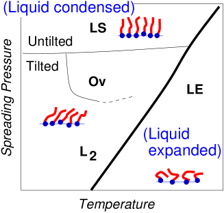
Figure 5: Generic phase diagram for fatty acid monolayers. (after Ref. kaganer_review). LE is the liquid expanded phase. In the L₂ phase and the Ov phase, the chains are tilted towards next-nearest and nearest neighbors, respectively. In the LS phase, they are on average untilted. Further phases are found at lower temperatures (not shown).

In order to describe such systems on a coarse-grained level, we model the amphiphiles as chains of $N$ “tail” beads with diameter $\sigma_{t}$, attached to a slightly larger “head” bead of diameter $\sigma_{h}>\sigma_{t}$. The water surface is represented by a planar surface at $z=0$, which repels the tail beads, and attracts the head bead.

More specifically, the model is defined as follows: The beads in the chains are connected by nonlinear springs with the potential

$$V_{S}(d)=\left\{\begin{array}[]{l c r}-\frac{k_{S}}{2}\;d_{S}^{2}\;\ln\Big{[}1-(d-d_{0})^{2}/d_{S}{}^{2}\Big{]}&\mbox{for}&|d-d_{0}|<d_{S}\\ \infty&\mbox{for}&|d-d_{0}|>d_{S}\end{array}\right.,$$ (1)

where $d$ is the length of the spring. This potential is constructed such that it is nearly harmonic in the center, at $d\approx d_{0}$, but diverges at $d=d_{S}$. Thus the distance between neighbor beads cannot take arbitrarily large values, which ensures that chains cannot cross each other. A potential with a logarithmic cutoff as in (1) is often called FENE-potential (Finite Extendible Nonlinear Elastic potential). In addition to this spring potential, chains are given a bending stiffness by virtue of a stiffness potential

$$V_{A}=k_{A}\cdot(1-\cos\theta),$$ (2)

which acts on the angle $\theta$ between subsequent springs and favors $\theta=0$ (straight chains). The parameter $k_{A}$ can then be tuned to control the conformational freedom of the chains and study the role of the chain entropy for the phase behavior.

Two beads $i$ and $j$ ($i,j=h$ or $t$) that are not direct neighbors in the same chain interact with a truncated and shifted Lennard-Jones potential,

$$V_{ij}(r)=\left\{\begin{array}[]{lcr}\epsilon\>\Big{(}\big{[}\sigma_{ij}/r\big{)}^{12}-2\big{(}\sigma_{ij}/r\big{)}^{6}+v_{ij}\Big{]}&\mbox{for}&r\leq R_{ij}\\ 0&\mbox{for}&r>R_{ij}\end{array}\right.,$$ (3)

where $\sigma_{ij}=(\sigma_{i}+\sigma_{j})/2$, the cutoff is $R_{tt}=2\sigma_{tt}$ for the tail beads, and $R_{ht}=\sigma_{ht}$, $R_{hh}=\sigma_{hh}$ for the other interactions, and the shifting parameter $v_{ij}$ is chosen such that $V_{ij}(r)$ is continuous at $r=R_{ij}$. It is easy to see that with this choice of the cutoff parameters, the interactions between tail beads are attractive, and all other interactions are purely repulsive.

Finally, we have to specify the interactions of beads with the surface. We have explored two types of surface potentials: First we used a model introduced by Haas et al [39], where the surface imposes rigid constraints: The head beads are confined to stay in the plane at $z=0$, and the tail beads are not allowed into the half-space $z<0$ [40, 41]. This model has the advantage of being very simple, however, it is unphysical in the sense that real water surfaces are not sharp on an atomic scale. Indeed, better agreement with the experimental phase diagram can be reached with softer surface potentials [42]. Here, head beads are subject to the potential

$$V_{h}(r)=\left\{\begin{array}[]{lcr}0&\mbox{for}&z<-0.5W\\ -{\epsilon_{s}}/{2}\>\ln\Big{[}1-(z+0.5W)^{2}/W^{2}\Big{]}&\mbox{for}&-0.5W<z<0.5W\end{array}\right.,$$ (4)

and tail beads to

$$V_{t}(r)=\left\{\begin{array}[]{lcr}-{\epsilon_{s}}/{2}\>\ln\Big{[}1-(z-0.5W)^{2}/W^{2}\Big{]}&\mbox{for}&-0.5W<z<0.5W\\ 0&\mbox{for}&z>0.5W\\ \end{array}\right..$$ (5)

with $W=1\sigma_{t}$ and $\epsilon_{s}=10\epsilon$. It turns out that the exact form of the surface potential is not important, almost identical results are obtained with $W=2\sigma_{t}$.

The other model parameters were $d_{0}=0.7\sigma_{t}$, $d_{S}=0.2\sigma_{t}$, and $k_{S}=100\epsilon$. The stiffness parameter $k_{A}$ was varied between $4.5\epsilon$ and $100\epsilon$. The head size was chosen $\sigma_{h}=1.1\sigma_{t}$ or $\sigma_{h}=1.2\sigma_{t}$, and the chain length was $N=7$ in most simulations.

This model was studied by Monte Carlo simulations at constant spreading pressure $P$: We considered $n$ chains with heads grafted in a planar parallelogram of variable size and shape, characterized by two side lengths $L_{x}$ and $L_{y}$ and one angle $\alpha$. The boundary conditions were periodic in the $xy$ plane, and free in the $z$ direction. The simulation algorithm included three elementary Monte Carlo moves:

• Single particle displacements

• Variations of $L_{x}$ or $L_{y}$, i. e., the whole configuration is stretched or squeezed in one direction. Care must be taken that this move satisfies detailed balance. For example, a move of the form $L\to L\delta$, where $\delta$ is uniformly distributed, cannot be applied without introducing a correction term in the probability for accepting the move. In contrast, the move $L\to L\exp(\delta)$ can be applied without correction. In our simulations, we varied $L$ in an additive way, $L\to L+\delta$ (rejecting moves that made $L$ negative).

• Shearing the box, i. e., variation of $\alpha$ while keeping the total area constant.

The moves were accepted or rejected according to the Metropolis prescription [44, 45, 47] with the effective Hamiltonian

$${\cal H}=E+PA-nNT\log A,$$ (6)

where $E$ is the (internal) energy, and $A$ is the area of the system. To speed up the simulations, we used cell lists and Verlet lists [46, 47]. Fig. 6 shows an example of a configuration snapshot.

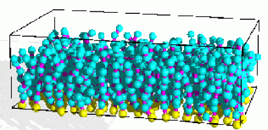
Figure 6: Snapshots of a monolayer in a system with $\sigma_{h}=1.1\sigma_{t}$, $k_{A}=10\epsilon$ and rigid constraints at the surface. ($T=4\epsilon/k_{B}$ and $P=50\epsilon/\sigma_{t}^{2}$) (Courtesy of C. Stadler).

To analyze the properties of the monolayer, one needs to define and monitor appropriate observables. One quantity of interest is the area per molecule. Fig. 7 shows typical temperature-area isobars. One clearly discerns a discontinuous jump, which moves to higher temperatures with increasing pressure.

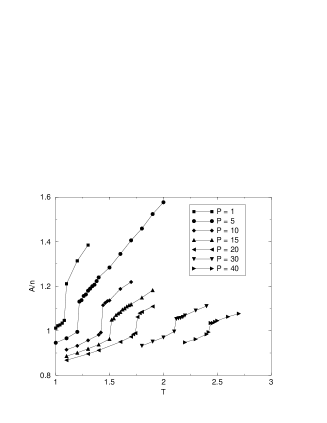
Figure 7: Area per molecule (in units $\sigma_{t}^{2}$) vs. temperature (in units $\epsilon/k_{B}$) in a system with $k_{A}=4.7\epsilon$, $\sigma_{h}=1.1\sigma_{t}$ and soft surface potentials. The spreading pressures are given in units of $\epsilon/\sigma_{t}^{2}$. From Ref. dominik_diplom.

The nature of this phase transition can be studied in more detail by inspecting the radial pair correlation functions and the hexagonal order parameter of two-dimensional melting,

$$\Psi_{6}=\bigg{\langle}\bigg{|}\frac{1}{6n}\sum_{j=1}^{n}\sum_{k=1}^{6}\exp(i6\phi_{jk})\bigg{|}^{2}\Big{\rangle}.$$ (7)

Here the sum $j$ runs over all heads of the system, the sum $k$ over the six nearest neighbors of $j$, and $\Phi_{jk}$ is the angle between the vector connecting the two heads and an arbitrary reference axis. The data for $\Psi_{6}$ which correspond to Fig. 7 are shown in Fig. 8. The hexagonal order parameter is nonzero in the low temperature phase, and jumps to a value close to zero at the transition. This indicates that the high temperature phase is liquid and the low temperature phase is hexatic or (quasi)crystalline.

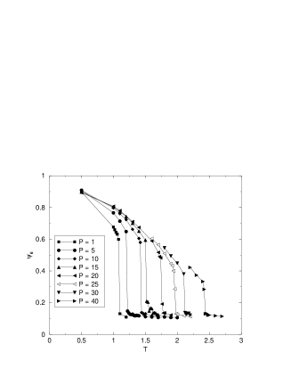
Figure 8: Order parameter $\psi_{6}$ vs. temperature (units $\epsilon/k_{B}$) for the same system as Fig. 7. From Ref. dominik_diplom.

A closer inspection of the ordered low-temperature region reveals that it can be subdivided in at least two regimes: At low pressures, the chains are collectively tilted in one direction, and at high pressure, they are on average untilted. The azimuthal symmetry breaking due to collective tilt order can be characterized by the order parameter

$$R_{xy}=\sqrt{\langle[x]^{2}+[y]^{2}\rangle},$$ (8)

where $[x]$ and $[y]$ denote the $x$ and $y$ components, respectively, of the head-to-end vector of a chain, averaged over all chains in one configuration, and $\langle\cdot\rangle$, the statistical average over all configurations. The values of $R_{xy}$ as a function of the pressure on two different isotherms are shown in Fig. 9.

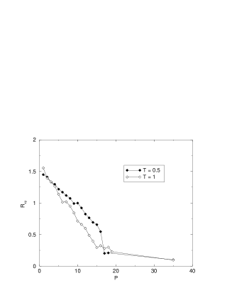
Figure 9: Tilt parameter $R_{xy}$ vs. pressure (in units $\epsilon/\sigma_{t}^{2}$) at two temperatures $T$ (in units $\epsilon/k_{B}$) for the same system as Fig. 7. From Ref. dominik_diplom.

The data for different temperatures and spreading pressures can be summarized in a phase diagram. An example for the system with soft potentials is shown in Fig. 10. This phase diagram has great similarity with the high temperature part of the experimental phase diagram in Fig. 5. At high temperature, we observe a disordered liquid expanded phase (LE). At low temperature two types of condensed phases are present – an untilted high-pressure phase (LS) and a tilted low-pressure phase (L₂/Ov). The temperature of the order-disorder transition increases with pressure, as in the experiment, and the pressure of the tilting transition between LS and L₂/Ov is almost independent of the temperature, again as in the experiment.

Figure 10: Phase diagram from Monte Carlo simulations of the monolayer model with $k_{A}=4.7\epsilon$, $\sigma_{h}=1.1\sigma_{t}$ and soft surface potentials. soft surface potentials in the plane of spreading pressure (units $\epsilon/k_{B}\sigma_{t}^{2}$) vs. temperature (units $\epsilon/k_{B}$). The chain stiffness is $k_{A}=4.7\epsilon$. LE denotes disordered phase, LS untilted ordered phase, and L₂/Ov ordered phase with tilt towards nearest or next-nearest neighbors (undetermined). From Refs. dominik,dominik_diplom

Thus we have established a minimal model which reproduces the main features of Langmuir monolayers in the vicinity of the main transition. At lower temperatures, the experimental phase diagram of fatty acids is much more complex than that of our model. This is not surprising. To reproduce phenomena like backbone ordering, the chains have to be modeled in much more detail than has been done here. On the other hand, the details of the low temperature portion of the experimental phase diagram depend strongly on the particular choice of the amphiphile. Our model was never designed to describe specific properties of fatty acids. It was designed to reproduce the main transition in amphiphile monolayers. This is achieved in a satisfactory way.

We can learn more about the main transition by playing with the model parameters and studying how this influences the phase behavior. For example, increasing the chain stiffness shifts the order/disorder transition to higher temperatures and the tilting transition to higher pressures [40]. The form of the surface potential (rigid or soft) is not important for the order/disorder transition, but it does influence the slope of the line of tilting transitions in pressure-area space [42]. Likewise, increasing the head group size by 10 % does not influence the order/disorder transition very much, but may affect the tilted phases quite dramatically [41]. All these observations can be summarized by the statement that the order/disorder transition is basically driven by the chains, whereas the tilting transitions result from an interplay between chains and head groups.

3.2 Bilayers

As mentioned earlier, lipid bilayers exhibit internal phase transitions which are very similar to those observed in monolayers. In other respect, however, they are fundamentally different. They do not form by adsorption on a pre-defined surface, instead, the lipids self-assemble spontaneously to a structure with planar geometry. As a result, bilayers are not strictly planar, but may curve around and undulate. In order to study membranes, one needs to define a model which reproduces self-assembly.

How can bilayer self-assembly be modeled? The simplest approach is to force amphiphiles into sheets by tethering the head groups to two dimensional surfaces [48, 49, 50, 51]. “Self-assembly” is then enforced by external constraints, with the obvious consequence that the head groups lose much of their translational degrees of freedom. In contrast, real self-assembled structures are held together by an interplay of amphiphile-amphiphile and amphiphile-solvent interactions. Coarse-grained models that reproduce spontaneous self-assembly must account for the presence of solvent one way or another. However, the solvent should be modeled with as little detail as possible, since the focus is still on the bilayers.

One possibility is to use the Smit model [26] mentioned in the introduction. The amphiphiles are modeled by chains of beads, and the solvent by beads of the same size. This model indeed reproduces bilayer self-assembly [52] and has been applied successfully by Goetz et al. to study shape fluctuations of model bilayers [53].

Unfortunately, even the simple Smit model still has the drawback that a substantial amount of computer time in simulations is spent on the uninteresting solvent. It is therefore desirable to have a model which does not include the solvent explicitly. This idea is not particularly eccentric, such models are commonly used in simulations of polymers in solvent. The effect of the solvent is then incorporated in the effective interactions between monomers. However, it is not a priori clear that effective (pair) interactions will be able to bring about something as complex as membrane self-assembly.

Indeed, it was only very recently that O. Farago [54] established a solvent-free molecular model for membranes. Amphiphiles are represented by rigid linear trimers, made of beads which interact through truncated Lennard-Jones interactions with carefully chosen interaction parameters. O. Farago showed that single bilayers remain (meta)stable in his model, that they exhibit an order-disorder phase transition as a function of the molecular area density, and that they even sustain pore formation. However, he also mentions that a lengthy “trial and error” process of fine tuning the Lennard-Jones parameters was necessary to achieve this impressive result.

In our own work [55], we propose a different, more robust approach, the “phantom solvent” model. Solvent particles are treated explicitly, but they interact only with the amphiphiles, not with one another. The amphiphiles perceive the solvent particles are soft beads of radius $\sigma_{s}=\sigma_{h}$. The bulk of the solvent region is simply an ideal gas. The amphiphiles are modeled exactly in the same way as in our previous monolayer model, except that the surface potentials (4) and (5) are of course eliminated and replaced by periodic boundary conditions. The model can be implemented in a straightforward way and studied by Monte Carlo simulations. We found that it produced stable bilayers at the first go, without any parameter tuning. Two examples of snapshots are shown in Fig. 11.

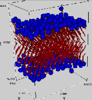
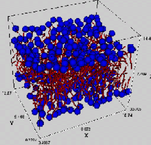
Figure 11: Snapshots of bilayers embedded in phantom solvent at pressure $P=1\epsilon/\sigma_{t}^{3}$ in the ordered state (left, temperature $T=0.9\epsilon/k_{B}$) and in the fluid state (right, $T=1.0\epsilon/k_{B}$). Solvent particles are not shown. ($\sigma_{h}=1.1\sigma_{t}$, $k_{A}=4.7\epsilon$)

The phantom solvent model has several advantages:

• It is computationally very efficient. The computational time spent on the phantom solvent is only a few percent of that spent on the amphiphiles, for any reasonable number of solvent beads. This is because only few pair interaction potentials have to be evaluated per solvent bead.

• The solvent has no local liquid structure. This is good, because we are not interested in the interplay between solvent and bilayer structure. If we intended to study this aspect, we would have to model the solvent (water!) in much more detail. Moreover, a structured solvent would introduce unwanted effective interactions between the bilayer and it’s periodic images in the normal direction.

• The phantom solvent has a simple physical interpretation. It probes the total free volume that is available to the solvent on the length scale $\sigma_{s}$. The self-assembly in our model is driven by the attractive interactions between the tails, and by the entropic effect that the solvents have more space when the amphiphiles are clustered together.

At the moment, the model still shares the handicap of all solvent-free models (and lattice models), that hydrodynamical interactions between the membranes and the solvent cannot be treated very easily. It might be possible to formulate dynamical equations for the phantom solvent which ensure that it behaves like a liquid and not like a gas. Otherwise, those who intend to study hydrodynamic effects might have to equip the solvent particles with a weak integrable potential, as is done in dissipative particle dynamics simulations. As long as we calculate static properties with Monte Carlo simulations, this is however not a problem.

After these general remarks, we turn back to the discussion of our particular amphiphile model. As mentioned before, it produced stable bilayers over a wide parameter range. The configuration snapshots of Fig. 11 demonstrate that the bilayers exhibit a low-temperature ordered phase and a high-temperature disordered phase. At even higher temperatures, they disintegrate. The phase transitions can be monitored, e. g., by inspecting the total nematic order parameter of amphiphiles or the area per lipid as a function of the pressure and temperature. A preliminary phase diagram is shown in Fig. 12. We note the similarity to the monolayer phase diagram of Fig. 10. This corroborates the assertion that monolayers are good model systems for membranes.

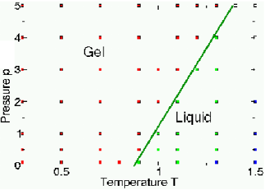
Figure 12: Preliminary phase diagram of bilayers in the phantom solvent model in the plane pressure (units $\epsilon/\sigma_{t}^{3}$) vs. temperature (units $\epsilon/k_{B}$). The model parameters are the same as in Fig. 10. Red points denote ordered membrane, and green points fluid membrane. At high temperatures (blue points), the membrane disintegrates.

3.3 Bilayer Stacks

Having discussed internal phase transitions in monolayers and bilayers, the logical next step would be to consider internal phase transitions in lamellar stacks. They exist, of course, but they are presumably not very different from those in single bilayers. Thus we will shift focus and concentrate on other aspects of membranes in this section: shape fluctuations and defects [56, 57, 58].

We consider a binary mixture of amphiphiles and solvent beads. The model shall not be described in full detail here. It was originally introduced by Soddemann et al [59, 60] and has some similarity with the Smit model. The elementary units are spheres with a hard core radius $\sigma$, which may have two types: “hydrophilic” or “hydrophobic”. Beads of the same type attract each other at distances less than $1.5\sigma$. “Amphiphiles” are tetramers made of two hydrophilic and two hydrophobic beads, and “solvent” particles are single hydrophilic beads.

Figure 13: Snapshot of a bilayer stack with 30720 amphiphiles and 30720 solvent beads. The “hydrophobic” tail beads are blue, the “hydrophilic” head beads are white, and the solvent beads are yellow.

The pressure and the temperature are chosen such that the system is in a fluid lamellar phase. More specifically, we study configurations with 5 or 15 stacked bilayers, which are swollen with 20 volume percent solvent. The simulations were done with constant pressure molecular dynamics, using a Langevin thermostat to maintain constant temperature. The constant pressure algorithm was designed such that the box dimensions parallel and perpendicular to the lamellae fluctuate independently, in order to ensure that the pressure is isotropic and the membranes have no surface tension. A configuration snapshot is shown in Fig. 13. It was produced by equilibration of an initial configuration with lamellar order, set up such that the lamellae were oriented perpendicular to the long axis (the $z$-axis) of the simulation box. We have checked with smaller systems that the lamellae self-assemble spontaneously if the initial configuration is disordered.

Our study aimed at analyzing shape fluctuations of the membranes and defects in the membranes. Therefore, the first nontrivial task was to determine the local positions of the membranes in the lamellar stack. This was done as follows:

• The simulation box was divided into $N_{x}N_{y}N_{z}$ cells. ($N_{x}=N_{y}=32$). Note that the size of the cells may vary between configurations because the dimensions of the box fluctuate in a constant pressure simulation.

• In each cell, the relative density of tail beads $\rho_{\mbox{\tiny tail}}(x,y,z)$ was calculated. It is defined as the ratio of the number of tail beads and the total number of beads.

• The hydrophobic space is defined as the space where the relative density of tail beads is higher than a given threshold $\rho_{0}$. The value of the threshold is roughly 0.7 (80 % of the maximum value of $\rho_{\mbox{\tiny tail}}$ and depends on the mesh size.

• The cells that belong to the hydrophobic space are connected to clusters. Two hydrophobic cells that share at least one vortex are attributed to the same cluster. Each cluster defines a membrane. This algorithm identifies membranes even if they have pores. At the presence of other membrane defects, additional steps have to be taken. (This happened very rarely in our system).

• For each membrane $n$ and each position $(x,y)$, the two heights $h_{n}^{\mbox{\tiny min}}(x,y)$ and $h_{n}^{\mbox{\tiny max}}(x,y)$, where the density $\rho_{\mbox{\tiny tail}}(x,y,z)$ passes through the threshold $\rho_{0}$, are determined. The mean position is defined as the average $h_{n}(x,y)=(h_{n}^{\mbox{\tiny min}}+h_{n}^{\mbox{\tiny max}})/2.$

The algorithm identifies membranes even if they have pores. A typical membrane conformation $h_{n}(x,y)$ is shown in Fig. 14. The statistical distribution of $h_{n}(x,y)$ can be analyzed and compared with theoretical predictions.

Figure 14: Typical conformation of a membrane position $h_{n}(x,y)$.

One of the simplest mesoscopic theories for fluctuations in membrane stacks is the “discrete harmonic model” [33]. It describes stacks of membranes without surface tension and assumes that the fluctuations are governed by two factors: The bending stiffness $K_{c}$ of single membranes, and the penalty for compressing the membranes, characterized by a compressibility modulus $B$. The free energy is given in harmonic approximation

$${\cal F}_{\mbox{\tiny DH}}=\sum_{n}\int_{A}dx\>dy\>\Big{\{}\frac{K_{c}}{2}(\frac{\partial^{2}h_{n}}{\partial x^{2}}+\frac{\partial^{2}h_{n}}{\partial y^{2}})^{2}+\frac{B}{2}(h_{n}-h_{n+1}+\bar{d})^{2}\Big{\}},$$ (9)

where $\bar{d}$ is the average distance between layers. This free energy functional is simple enough that statistical averages can be calculated exactly. For example, the transmembrane structure factor which describes correlations between membrane positions in different membranes is given by [57]

$$s_{n}(q)=\langle h_{m}({\bf q})^{*}h_{m+n}({\bf q})\rangle=s_{0}(q)\>\Big{[}1+\frac{X}{2}-\frac{1}{2}\sqrt{X(X+4)}\Big{]}^{n},$$ (10)

where $h_{n}({\bf q})$ is the Fourier transform of $h_{n}(x,y)$ in the $(x,y)$-plane and $X=q^{4}K_{c}/B$ is a dimensionless parameter. The function $s_{0}(q)$ can also be given explicitly [57]. We can test the prediction (10) by simply plotting the ratio $s_{n}/s_{0}$ vs. $q$ for different $n$. The functional form of the curves should be given by the expression in the square brackets, with only one fit parameter $K_{c}/B$. Fig. 15 shows our simulation data. The agreement with the theory is very good over the whole range of $q$. Hence the discrete harmonic model, a mesoscopic theory, describes the membrane fluctuations in our molecular way in a satisfactory way.

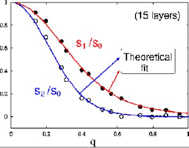
Figure 15: Ratios of transmembrane structure factors $s_{1}/s_{0}$ and $s_{2}/s_{0}$ vs. in-plane wavevector $q$ in units of $\sigma^{-1}$. The solid lines correspond to a theoretical fit to Eq. (10) with one (common) fit parameter $K_{c}/B$.

Moreover, our analysis provides a value for the phenomenological parameter $K_{c}/B$. By combining it with the analyses of other quantities, it is possible to determine $K_{c}$ and $B$ separately. This establishes a bridge between the molecular and the mesoscopic description.

Next we turn to discuss the membrane defects in the lamellar stack. On principle, one can have three types of topological point defects in membranes: necks, pores, and passages. In our system, necks and passages were extremely rare, and we did not collect enough data to be able to analyze them statistically. Thus we will focus on the pores here.

As we have already mentioned, the properties of pores determine the permeability of a membrane. A number of atomistic and coarse grained simulation studies have therefore addressed pore formation [31, 61, 62, 63], mostly in membranes under tension. In contrast, the membranes in our lamellar stack have no surface tension. As we shall see, this affects the characteristics of the pores quite dramatically.

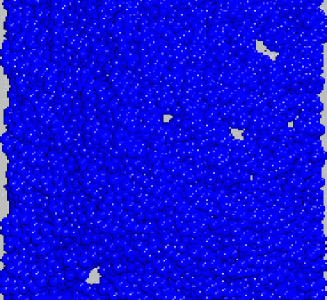
Figure 16: Snapshot of the hydrophobic beads in a single bilayer (top view).

Fig. 16 shows a snapshot of a hydrophobic layer which contains a number of pores. These pores have nucleated spontaneously. They “live” for a while, grow and shrink without diffusing too much, until they finally disappear. Most pores close very quickly, but some large ones stay open for a long time.

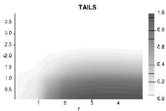
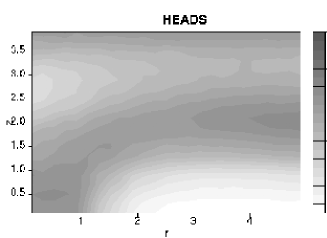
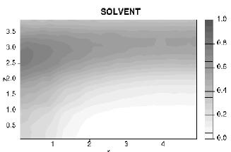
Figure 17: Density profiles of tail beads, head beads, and solvent beads as a function of the distance from the center of the pore in radial in-plane direction $r$ and normal direction $z$.

We will first analyze the local membrane structure in the vicinity of a pore. Fig. 17 shows average composition profiles of tail beads, head beads and solvent beads as a function of the in-plane distance from the center of the pore, $r$, and the normal out-of-plane coordinate, $z$. These averages were performed with data from pores with surface areas between 4 and 16 $\sigma^{2}$. The pictures demonstrate that the amphiphiles rearrange themselves at the pore edge, so that solvent beads in the pore center are exposed mainly to head beads. Such a pore is called hydrophilic. In previous simulations, both hydrophilic and hydrophobic pores have been reported, depending on the system under consideration.

Whereas the local composition profiles at the pore edge depend on the model, other structural properties of pores on larger scales are presumably generic and can again be described by simple mesoscopic theories. For example, the simplest Ansatz for the free energy of a pore with the area $A$ and the contour length $c$ has the form [34]

$$E=E_{0}+\lambda\>c-\gamma\>A,$$ (11)

where $E_{0}$ is a core energy, $\lambda$ a material parameter called line tension, and $\gamma$ the surface tension. The last term accounts for the reduction of energy due to the release of surface tension in a stretched membrane. In our case, the surface tension is zero ($\gamma=0$), and the last term vanishes. The second term describes the energy penalty at the pore rim. If this simple free energy model is correct, the pore shapes should be distributed according to a Boltzmann distribution

$$P(c)\propto\exp(-\lambda c).$$ (12)

This can be tested in the simulation. Fig. 18 shows a histogram of contour lengths $P(c)$. The bare data do not reflect the expected exponential behavior. Either the Ansatz (11) is wrong, or we have not used it correctly.

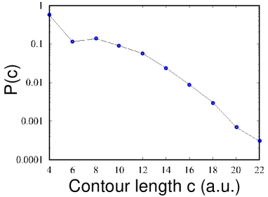
Figure 18: Distribution of pore contours in a semi-logarithmic plot.

Indeed, a closer look reveals that Eq. (12) disregards an important effect: The “free energy” (11) gives only local free energy contributions, stemming from local interactions and local amphiphile rearrangements. In addition, one must also account for the global entropy of possible contour length conformations. Therefore, we have to evaluate the “degeneracy” of contour lengths $g(c)$, and test the relation

$$P(c)\propto g(c)\exp(-\lambda c).$$ (13)

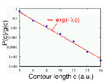
Figure 19: Distribution of pore contours, divided by the degeneracy function $g(c)$.

Fig. 19 demonstrates that this second Ansatz describes the data very well. From the linear fit to the data, one can extract a value for the line tension $\lambda$. Thus we have again established a bridge between the molecular simulation model and a mesoscopic theory.

If the model (11) is correct, it makes a second important prediction: Since the free energy only depends on the contour length, pores with the same contour length are equivalent and the shapes of these pores should be distributed like those of two dimensional ring polymers. In particular, they are not round, but have a fractal structure. From polymer theory, one knows that the size $R_{g}$ of a two dimensional self-avoiding polymer scales roughly like $R_{g}\propto N^{3/4}$ with the polymer length $N$. In our case, the “polymer length” is the contour length $c$. Thus the area $A$ of a pore should scale like

$$A\propto R_{g}^{2}\propto(C^{3/4})^{2}=C^{3/2}.$$ (14)

Fig. 20 shows that this is indeed the case.

Figure 20: Pore area vs. contour length (arbitrary units).

Many other properties of the pores can be investigated, e. g., pore distributions, the dynamical evolution of pores, pore life times [56, 58]. Nevertheless, we shall stop here. We hope that our brief discussion has conveyed an idea how a coarse-grained molecular simulation help to test and justify mesoscopic theories, and to establish a connection between molecular and mesoscopic descriptions of amphiphilic systems.

4 Outlook

Simulations like those presented here are only a very first step towards understanding the properties of membranes. First, real biomembranes are not pure systems, but contain a mixture of many different lipids, with saturated or unsaturated chains, with charged or neutral heads etc. Second, biomembranes are filled with proteins. Typical biomembranes are not homogeneous, but compartmented into several regions with different lipid and protein composition. Furthermore, biomembranes have a complex environment, which influences the membrane properties. Finally, biomembranes are not equilibrium structures. They contain active proteins, and they are surrounded by an ever changing environment.

These many complications seem discouraging. We hope to have shown that a systematic approach, where the different aspects of membranes are studied one by one with appropriated idealized models, can be rewarding. Still, much remains to be done. Computer simulations of membranes and biomembranes will certainly be an active and lively research area for a long time.

References

- [1] J Israelachvili, Intermolecular and Surface Forces (Academic Press, London, 1991)
- [2] G. Gompper and M. Schick, Self-Assembling Amphiphilic Systems Vol. 16 of Phase Transitions and Critical Phenomena, C. Domb and J. L. Lebowitz Eds (Academic press, London, 1994).
- [3] K. V. Schubert, \JournalBer. Bunseng. Phys. Chemie1001901996.
- [4] R. B. Gennis, Biomembranes (Springer Verlag, New York, 1989).
- [5] V. M. Kaganer, H. Möhwald, and P. Dutta, \JournalRev. Mod. Phys.717791999.
- [6] D. A. Antelmi and P. Kekicheff, \JournalJ. Phys. Chem. B10181691997.
- [7] C. Münster, T. Salditt, M. Vogel, R. Siebrecht, and J. Peisl, \JournalEurophys. Lett.464861999.
- [8] T. Salditt, C. Münster, U. Mennicke, C. Ollinger, and G. Fragneto, \JournalLangmuir1977032003.
- [9] E. Freyssingeas, D. Antelmi, P. Kekicheff, P. Richetti, and A. M. Bellocq, \JournalEurop. Phys. J. B91231999.
- [10] I. Koltover, J. O. Rädler, T. Salditt, K. J. Rothschild, and C. R. Safinya, \JournalPhys. Rev. Lett.8231841999.
- [11] C. Münster, J. Lu, S. Schinzel, B. Bechinger, and T. Salditt, \JournalEurop. Bioph. J.286832000.
- [12] J. O. Rädler, I. Koltover, T. Salditt, and C. R. Safinya, \JournalScience2758101997.
- [13] F. Artzner, R. Zantl, G. Rapp, and J. O. Rädler, \JournalPhys. Rev. Lett.8150151998.
- [14] H. G. Döbereiner, \JournalCurr. Opin. Coll. Int. Phys.52562000.
- [15] H.M. McConnell, \JournalAnn. Rev. Phys. Chem.421711991.
- [16] C. M. Knobler and R. C. Desai, \JournalAnn. Rev. Phys. Chem.432071991.
- [17] S. A. Safran, Statistical Thermodynamics of Surfaces, Interfaces and Membranes (Addison-Wesley, Reading, Massachusetts, 1994).
- [18] R. Lipowsky, \JournalJ. Phys. II218251992.
- [19] H. G. Döbereiner, J. Käs, D. Noppl, and I. Sprenger, \JournalBiophys. J.6513961993.
- [20] S. Yamamoto and S. Hyodo, \JournalJ. Chem. Phys.11879372003.
- [21] D. A. Brown and E. London, \JournalAnn. Rev. Cell. Dev. Biol.141111998.
- [22] S. Safran, T. Kuhl, and J. Israelachvili, \JournalBiophys. J.818592001.
- [23] R. G. Larson, L. E. Scriven, and H. T. Davis, \JournalJ. Chem. Phys.8324111985.
- [24] T. B. Liverpool, Ann. Rev. Comp. Phys. IV, D. Stauffer Edt., pp. 317-358 (World Scientific, Singapore, 1996).
- [25] R. G. Larson, \JournalJ. Physique II614411996.
- [26] B. Smit, A. G. Schlijper, L. A. M. Rupert, N. M. van Os, \JournalJ. Phys. Chem.9469331990.
- [27] D. A. Pink, T. J. Green, and D. Chapman, \JournalBiochemistry193491980.
- [28] A. Caillé, D. Pink, F. de Verteuil, and M. Zuckermann, \JournalCan. J. de Physique585811980.
- [29] B. Dammann, H. C. Fogedby, J. H. Ipsen, C. Jeppesen, K. Jorgensen, O. G. Mouritsen, J. Risbo, M. C. Sabra, M. M. Sperotto, M. J. Zuckermann, Handbook of Nonmedical Applications of Liposomes, Vol. 1, p. 85, D. D. Lasic, Y. Barenholz Eds. (CRC press, 1995).
- [30] G. Gompper and D. M. Kroll, \JournalJ. Phys.: Cond. Matt.987951997.
- [31] M. Müller, K. Katsov, and M. Schick, \JournalJ. Chem. Phys.11623422002.
- [32] R. Holyst, \JournalPhys. Rev. A4436921991.
- [33] N. Lei, C. R. Safinya, and R. F. Bruinsma, \JournalJ. Phys. II511551995.
- [34] J. Lister, \JournalPhys. Lett.53A1931975.
- [35] J. Shillcock and U. Seifert, \JournalBiophys. J.7417541998.
- [36] A. M. Bibo and I. R. Peterson, \JournalAdv. Mater.23091990.
- [37] I. R. Peterson, V. Brzezinsky, R. M. Kenn, and R. Steitz, \JournalLangmuir829951992.
- [38] G. A. Overbeck and D. Möbius, \JournalJ. Phys. Chem.9779991993.
- [39] F. M. Haas and R. Hilfer, \JournalJ. Chem. Phys.10338591996.
- [40] C. Stadler, H. Lange, and F. Schmid \JournalPhys. Rev. E5942481999.
- [41] C. Stadler and F. Schmid \JournalJ. Chem. Phys.11096971999.
- [42] D. Düchs and F. Schmid \JournalJ. Phys.: Cond. Matt.1348532001.
- [43] D. Düchs, Diplomarbeit Universität Mainz, 1999.
- [44] K. Binder and D. W. Heermann, Monte Carlo Simulation in Statistical Physics: An introduction (Springer, Berlin, 1990).
- [45] D. P. Landau and K. Binder, A Guide to Monte Carlo Simulations in Statistical Physics (Cambridge University Press, Cambridge, 2000).
- [46] M. P. Allen and D. J. Tildesley, Computer Simulations of Liquids (Oxford University Press, Oxford, 1989).
- [47] D. Frenkel and B. Smit, Understanding Molecular Simulation (Academic Press, London, 1996).
- [48] D. Harries and A. Ben-Shaul, \JournalJ. Chem. Phys.10616091997.
- [49] A. Baumgärtner, \JournalJ. Chem. Phys.103106691995.
- [50] A. Baumgärtner, \JournalBiophys. J.7112481996.
- [51] T. Sintes and A. Baumgärtner, \JournalBiophys. J.7322511997.
- [52] R. Goetz and R. Lipowsky, \JournalJ. Chem. Phys.10873971998.
- [53] R. Goetz, G. Gompper, and R. Lipowsky, \JournalPhys. Rev. Lett.822211999.
- [54] O. Farago, \JournalJ. Chem. Phys.1195962003.
- [55] O. Lenz and F. Schmid, J. Mol. Liquids, in preparation (2003).
- [56] C. Loison, Dissertation, ENS Lyon and Universität Bielefeld, 2003.
- [57] C. Loison, M. Mareschal, K. Kremer, and F. Schmid, J. Chem. Phys., in press (2003).
- [58] C. Loison, M. Mareschal, and F. Schmid, in preparation (2003).
- [59] T. Soddemann, B. Dünweg, and K. Kremer, \JournalEurop. Phys. J. E64092001.
- [60] H.-X. Guo, K. Kremer, and T. Soddemann, \JournalPhys. Rev. E660615032002.
- [61] M. Müller, M. Schick, \JournalJ. Chem. Phys.11623421996.
- [62] S. Marrink, F. Jähning, and H. Berendsen, \JournalBiophys. J.716321996.
- [63] D. Zahn, J. Brickmann, \JournalChem. Phys. Lipids352412002.