MS-TP-04-10 cond-mat/0405673
Profile and width of rough interfaces

Abstract

In the context of Landau theory and its field theoretical refinements, interfaces between coexisting phases are described by intrinsic profiles. These intrinsic interface profiles, however, are neither directly accessible by experiment nor by computer simulation as they are broadened by long-wavelength capillary waves. In this paper we study the separation of the small scale intrinsic structure from the large scale capillary wave fluctuations in the Monte Carlo simulated three-dimensional Ising model. To this purpose, a blocking procedure is applied, using the block size as a variable cutoff, and a translationally invariant method to determine the interface position of strongly fluctuating profiles on small length scales is introduced. While the capillary wave picture is confirmed on large length scales and its limit of validity is estimated, an intrinsic regime is, contrary to expectations, not observed.
KEY WORDS: Interfaces, roughening, capillary waves, Monte Carlo

1 Introduction

Under suitable conditions systems of statistical mechanics can exhibit coexistence of different phases which are separated spatially by interfaces. Structure and properties of such interfaces have been investigated both experimentally and theoretically, and still offer problems for current research. Near critical points several interfacial properties are expected to show universal behaviour.

Since the 19th century, there has been continuous interest in the theoretical description of interfaces [1, 2, 3, 4]. Traditionally, the interface has been described by mean field theories and their refinements [5, 6, 7] as an “intrinsic” continuous profile with a width proportional to the bulk correlation length.

The existence of the interface, however, breaks the translational invariance of the system, resulting in long-wavelength capillary wave fluctuations of the interface position as Goldstone-modes. These fluctuations are neglected by mean field theory which assumes a flat interface, but they strongly influence the interfacial properties. According to capillary wave theory [8, 9], the interface width, for example, depends logarithmically on the system size and diverges in the limit of an infinite system.

Mean field and capillary wave theory can be viewed as a small-scale and large-scale description of the interface, respectively, and then be combined in the “convolution approximation” [4, 1]. In this picture the interface is described as an intrinsic profile which is centered around a two-dimensional surface subject to capillary wave fluctuations.

While capillary wave behaviour has been observed in many systems (e.g. experimentally on liquid-vapor interfaces [10] and polymer mixtures [11], in simulations of polymer mixtures [12] and of the Ising model [13, 14, 15]), the mean field behaviour is difficult to access as the intrinsic profile - if it has a well-defined meaning at all - is broadened by the capillary wave fluctuations.

The concept of intrinsic versus large-scale interface structure has so far not been defined unambiguously outside a given theory. There is no clear “snapshot” definition of an interface, which always shows overhangs, islands, clusters which may be as well assigned to the phase-separating interface region as to the fluctuation structure of the neighbouring homogeneous phases.

In this paper the attempt is made to separate the intrinsic structure from the influence of the capillary waves via a blocking procedure reminiscent of the Kadanoff block spin method of renormalization group theory. The system of size $L\times L\times D$ with an interface perpendicular to the $D$-direction is divided into blocks of size $B\times B\times D$. The different length scales are separated by using the block size $B$ as a variable cutoff. To calculate the interface position of the strongly fluctuating interface profiles on small length scales, we implement a method which respects translational invariance (in contrast to various other approaches in the literature). In this way, the local interface position, the interface profile and the interface width can be studied on the different length scales, thereby allowing a direct test of the convolution approximation and of the limits of validity of the capillary wave theory and of the mean field theory. It is found that on large length scales, the capillary wave picture is consistent with the data.

On small length scales, however, contrary to expectations we cannot identify an intrinsic interface profile with a width of the order of the correlation length. For the case of the Ising model under study the concept of the intrinsic profile is thus called into question.

An approach based on blocking has already been used by Weeks [16] for liquid-vapour interfaces in order to derive the capillary wave model from a microscopic model Hamiltonian, thereby reconciling mean field and capillary wave theory as small-scale and large-scale interface descriptions, respectively. In the context of Monte Carlo simulations a procedure similar to the one used in this paper has been applied by Werner et al. [12] to homopolymer interfaces, finding consistency of their data with the convolution approximation.

2 Theoretical description of the interface
profile

2.1 Intrinsic interface profile

Interfaces can be described in mean field theory by a continuous profile $\phi(x)$ representing the difference between the concentrations of the two coexisting phases. In the framework of Landau theory and its field theoretical extensions the profile function plays the role of a local order parameter. Near the critical temperature the free energy density is written as [17]:

$$\mathcal{L}=\frac{1}{2}(\partial\phi(x))^{2}+V(\phi(x))$$ (1)

with the double-well potential

$$V(\phi)=\lambda(\phi^{2}-1)^{2}\,.$$ (2)

The minima of this potential correspond to the two homogeneous phases, whose densities have been normalized to $\pm 1$ for simplicity.

Minimization of the free energy density (1) with boundary conditions appropriate for an interface perpendicular to the $z$-axis leads to the typical hyperbolic tangent mean field profile [6]

$$\phi(z)=\tanh\left(\frac{1}{2\xi_{0}}(z-h)\right)$$ (3)

with a width proportional to the mean field correlation length $\xi_{0}$, which diverges near the critical point with exponent 1/2. The parameter $h$ specifies the location of the interface which is arbitrary due to translational invariance.

Corrections due to fluctuations of the order parameter field can be calculated systematically in renormalized perturbation theory. In the “local potential approximation” only corrections to the local potential $V(\phi)$ are taken into account, whereas contributions involving higher powers of derivatives are neglected. The resulting interface profile is of the form $\phi(z)=f((z-h)/2\xi)$, where the width is now proportional to the physical correlation length $\xi$, which diverges near the critical point with exponent $\nu$. This corresponds to the scaling form proposed by Fisk and Widom [7]. To lowest order the profile function $f$ is equal to the mean field profile function, $f=\tanh$. In higher orders, corrections to the potential $V(\phi)$ due to perturbative loop contributions modify the mean field profile [18]. We do, however, not consider them as they are numerically small and can be neglected in our context.

The interface profile

$$\phi(z)=\tanh\left(\frac{1}{2\xi}(z-h)\right)\,,$$ (4)

in lowest order of the local potential approximation is to be distinguished from the mean field profile. It represents a refinement of Landau theory that is consistent with scaling [7] and holds near the critical point.

In the local potential approximation long wavelength fluctuations are not fully taken into account. Consequently the profile (4) does not contain the effects of capillary waves, which are discussed in the following section. The function above thus represents an intrinsic interface profile.

2.2 Capillary wave theory

Translational invariance is broken by the presence of the interface. The Goldstone bosons associated with this broken symmetry are long wavelength excitations of the interface position, which have vanishing energy cost in the infinite wavelength limit [19]. These capillary waves strongly influence interfacial properties like the interface width but are neglected by mean field theory which assumes a flat interface. In capillary wave theory, as introduced by Buff et al. [8], bubbles, overhangs and any continuous density variations of the interface are neglected. The local interface position is parameterized by a single-valued function $h(x,y)$, describing the interface as a fluctuating membrane. The free energy cost of capillary waves is basically due to the increase in interface area against the reduced interface tension $\sigma$. Thus the capillary wave free energy (multiplied by the inverse temperature $\beta$) is [2]

$$\beta\mathcal{H}=\sigma\!\int\!\!dxdy\left[\sqrt{1+(\nabla h)^{2}}-1\right]\approx\frac{\sigma}{2}\int\!\!dxdy\,(\nabla h)^{2}\,,$$ (5)

where $|\nabla h|\ll 1$, i.e. long wavelength and small amplitude, has been assumed. The Gaussian nature of the capillary wave model allows analytic calculation of thermal averages. The local interface position is distributed according to a Gaussian distribution

$$P(h)=\langle\delta(h(x,y)-h)\rangle=\frac{1}{\sqrt{2\pi}\,s}\,\mathrm{e}^{-h^{2}/2s^{2}}$$ (6)

with variance

$$s^{2}=\langle h^{2}\rangle=\frac{1}{2\pi\sigma}\int\!\!dq\,\frac{1}{q}=\frac{1}{2\pi\sigma}\ln\frac{L}{B_{\mathrm{cw}}}\,.$$ (7)

In order to avoid divergence of the integral, a lower cutoff $2\pi/L$ and an upper cutoff $2\pi/B_{\mathrm{cw}}$ have been introduced. Here $L$ is the system size, which determines the maximal allowed wavelength and provides a natural lower cutoff for the capillary wave spectrum. The cutoff length $B_{\mathrm{cw}}$, which is so far arbitrary, sets the scale below which capillary wave theory ceases to be valid. As there should be no capillary waves with wavelength smaller than the intrinsic width of the interface, $B_{\mathrm{cw}}$ should be of the order of the correlation length. The factor $2\pi$ in the lower cutoff is due to periodic boundary conditions and has also been introduced in the upper cutoff for convenience. The phenomenological capillary wave model thus requires two inputs: the macroscopic interface tension $\sigma$ and the cutoff $B_{\mathrm{cw}}$. While the interface tension near the critical temperature is known from scaling [4], the cutoff $B_{\mathrm{cw}}$ is unknown.

In the capillary wave picture the instantaneous interface profile is a sharp step function between the two phases. Nevertheless, in the thermal average the capillary wave fluctuations produce a continuous density profile

$$\rho(z)=\int\!\!dh\ \mathrm{sgn}(z-h)\,P(h)=\mathrm{erf}\left(\frac{z}{\sqrt{2}s}\right)$$ (8)

with a finite width whose square is proportional to the variance $s^{2}$ (7) and thus to the logarithm of the system size $L$. In other words, the apparent width of the interface depends on the length scale on which the interface is studied and diverges in the thermodynamic limit.

2.3 Convolution approximation

The two different descriptions of the interface profile - intrinsic profile and capillary wave theory - can be reconciled by adopting the view that the intrinsic profile describes the interface on a microscopic scale of the order of the correlation length, while capillary wave theory describes the macroscopic interface fluctuations of wavelengths much larger than the correlation length. Neglecting the coupling of the capillary wave fluctuations to the intrinsic interfacial structure, the interface can be viewed as a fluctuating capillary wave theory membrane $h(x,y)$, to which an intrinsic profile $\phi(z)$ is “attached”. In this way an instantaneous profile $\phi(z-h(x,y))$ is obtained. Performing the thermal average over the capillary waves, the “apparent” profile is given by the convolution

$$m(z)=\int\!\!dh\,\phi(z-h)P(h).$$ (9)

In this convolution approximation, the intrinsic profile $\phi$ is thus broadened by capillary wave fluctuations. The broadening increases with the system size according to Eqs. (6) and (7) corresponding to the fact that in a larger system more capillary waves are allowed.

2.4 Interface width

The interface width cannot be defined in a unique way, and various definitions have been used in the literature (see e.g. refs. [4], [8] and [14]). For numerical purposes, a suitable definition of the squared interface width is the second moment of a weight function which is proportional to the gradient of the interface profile m:

$$w^{2}=\frac{\int\!\!dz\,z^{2}m^{\prime}(z)}{\int\!\!dz\,m^{\prime}(z)}.$$ (10)

Due to the linearity of this definition and of the convolution approximation (9), the squared width $w^{2}$ of the convolution profile $m$ is simply the sum of the intrinsic width squared $w_{\mathrm{int}}^{2}$ of the intrinsic profile $\phi$, Eq. (4), and of the capillary width squared $w_{\mathrm{cw}}^{2}=s^{2}$ of the capillary wave profile $\rho$, Eq. (8):

$$w^{2}_{\mathrm{ca}}=w_{\mathrm{int}}^{2}+w_{\mathrm{cw}}^{2}=\frac{\pi^{2}}{3}\xi^{2}+\frac{1}{2\pi\sigma}\ln\frac{L}{B_{\mathrm{cw}}}.$$ (11)

This expression shows the broadening of the intrinsic profiles by capillary waves. It can be cast into a temperature-independent form by expressing all lengths in units of twice the correlation length:

$$\hat{w}^{2}_{\mathrm{ca}}=\left(\frac{w}{2\xi}\right)^{2}=\hat{w}^{2}_{\mathrm{int}}+\hat{w}^{2}_{\mathrm{cw}}=\frac{\pi^{2}}{12}+\hat{A}_{\mathrm{cw}}\log_{2}\frac{\hat{L}}{\hat{B}_{\mathrm{cw}}},$$ (12)

where $\hat{L}=L/2\xi$, $\hat{B}_{\mathrm{cw}}=B_{\mathrm{cw}}/2\xi$. Here the slope

$$\hat{A}_{\mathrm{cw}}=\frac{\ln 2}{8\pi\sigma\xi^{2}}=0.265(2)$$ (13)

contains the the universal constant $\sigma\xi^{2}=0.1040(8)$ [20, 21]. We also considered other definitions of the interface width, e.g. with a weight function proportional to $(m^{\prime}(z))^{2}$, but the results to be discussed below are not altered significantly.

3 Monte Carlo calculation

3.1 Monte Carlo setup

In experiments or Monte Carlo simulations of systems with interfaces the observed interface profile and width are the total ones, including the effects of the intrinsic structure as well as of the capillary waves. In order to investigate the question whether the intrinsic structure can be separated from the effects of capillary waves, suitable observables have to be constructed. We have studied this question by means of Monte Carlo simulations of the three-dimensional Ising model, which is in the same universality class as three-dimensional binary mixtures. The results allow to test the predictions from capillary wave theory and the validity of the convolution approximation.

In the simulations a cubic lattice of size $L\times L\times D$ is used, with spins $s(x,y,z)\in\{\pm 1\}$ on each lattice site $(x,y,z)$. The presence of an interface is enforced by antiperiodic boundary-conditions in the $z$-direction, while the boundary conditions in the $x,y$-directions are periodic. The lattice sizes are varied from $L=32$ to 512 and from $D=50$ to 180. To reduce critical slowing down, the Single-Cluster-Wolff algorithm [22] is used to allow simulations at reduced temperatures $t=(T-T_{c})/T_{c}=-0.05$, $-0.01$ and $-0.004$, corresponding to correlation lengths $\xi=1.65$, $4.56$ and $8.13$ in lattice units, respectively.

In order to analyze the interface on different length scales a blocking procedure is applied. The system is split into columns of block size $B\times B$ and of length $D$. The block size $B$ will later be varied to allow for systematic analysis. In each block $i$ a local block profile is calculated by averaging over the lateral coordinates in the block:

$$m_{i}(z)=\frac{1}{B^{2}}\sum_{x,y\in\mathrm{Block}\ i}s(x,y,z)\,.$$ (14)

3.2 Local interface position

Due to strong thermal fluctuations near the critical point the interface position for this profile is not well-defined. Various methods have been proposed to determine the interface position (see e.g. refs. [15], [23] and [24]) and applied to total interface profiles, i.e. for the profile (14) at $B=L$. These methods, however, are not appropriate for our purpose, because they either neglect bulk fluctuations, whose contributions we want to take into account fully, or they suffer from a lack of translational invariance: If the interface is, due to interface wandering, not in the middle of the system, the fluctuations above and below the interface do not average out, leading to a biased value for the interface position. This bias can be neglected for profiles on sufficiently large length scales, i.e. for block profiles with sufficiently large $B$, but not for the strongly fluctuating profiles on smaller length scales $B$.

To solve this problem, a translationally invariant method to determine the interface position is proposed [25]. Because of the periodic/antiperiodic boundary conditions, the Ising lattice is wrapped to a torus. The antiperiodicity is implemented by taking the couplings between nearest neighbours $s(x,y,z)$ and $s(x,y,z+1)$ to be negative for a particular value of $z=z_{a}$. Superficially, the choice of $z_{a}$ appears to break translation invariance along the $z$-direction. This is, however, not the case. Under a shift of $z_{a}$ the Hamiltonian remains invariant, if at the same time those spins, which cross the plane of antiperiodicity, are flipped. Consequently translation invariance remains a symmetry. Observables should be constructed in such a way that they also respect translation invariance. Translational invariance of our method to determine the interface position is achieved in the following way. The antiperiodicity point $z_{a}$ is shifted through the system successively. The values of the block profiles $m_{i}(z)$, which cross the antiperiodicity plane $z=z_{a}$, change signs appropriately. For a monotone interface profile function $m(z)$, all values would get the same sign, if $z_{a}$ coincides with the center of the interface. Correspondingly, we define the location $z$ of the interface to be that value of $z_{a}$, which makes the number of values of $m_{i}(z)$ having the same sign maximal, i.e. being mostly positive or mostly negative. Mathematically this point can be determined as the maximum of $|\sum_{z}m_{i}(z)|$. In this way, one assures that the fluctuations near the interface determine the precise location of the interface position. It would also be possible to use the minimum of $|\sum_{z}m_{i}(z)|$, which is attained when the interface is located opposite of $z_{a}$. In this case, however, fluctuations deep in the bulk phase opposite (on the torus) to the interface position would account for the precise location of the interface position, which is physically less meaningful.

This boundary shift method very successfully determines the interface positions for strongly fluctuating profiles even on rather small length scales $B$, but of course fails for extremely small length scales $B=1,2,3$, where the profiles $m_{i}(z)$ are still reminiscent of their Ising nature with only two allowed values $\pm 1$ and thus do not possess a well-defined interface position at all. This will result in Ising lattice artefacts for extremely small block sizes in the later discussion. But as neither of the interface models discussed in section 2 applies on a microscopic scale, this deficiency of the method does not prevent a test of the models.

3.3 Interface profile

In order to obtain the interface profile without fluctuations on length scales larger than $B$, the block profiles $m_{i}(z)$ can now be shifted such that the interface position is in the middle of the system. Note that values that pass the antiperiodic boundary conditions change sign (spin flip). To assure that the profile values above the interface are predominantly positive, an overall sign change is applied if necessary. The shift procedure corresponds to a measurement in a moving frame that is wandering with the local interface, i.e. to an elimination of the zero mode within the block. One can now take the block and Monte Carlo average over the block profiles $m_{i}(z)$ to obtain the local interface profile $m(z)$ on the scale of the block length $B$. This profile corresponds to the apparent profile (9) of the convolution approximation measured on a length scale of the block size $B$.

The interface width of the profile is determined via a discretized gradient analysis corresponding to Eq. (10). Let the $z$-coordinates take the values $1,2,\ldots,D$. An auxiliary coordinate $t=z-D/2$ is introduced which labels the positions between adjacent lattice sites and is centered about the middle of the system, assuming the values $-D/2+1,-D/2+1,\ldots,D/2-1$. A normalized gradient is then defined by

$$p(t)=\frac{1}{N}\left|m\left(t+\frac{D}{2}+1\right)-m\left(t+\frac{D}{2}\right)\right|$$ (15)

with the normalization

$$N=\sum_{t}\left|m\left(t+\frac{D}{2}+1\right)-m\left(t+\frac{D}{2}\right)\right|\,.$$ (16)

The interface width is the second moment of this weight function:

$$w^{2}=\sum_{t}t^{2}\,p(t)-\bigg{(}\sum_{t}t\,p(t)\bigg{)}^{2}.$$ (17)

So far each block has been considered as an Ising system of size $B\times B\times D$ in its own right, for which the same measurements as for a total Ising system have been made. In this way all fluctuations of wavelengths larger than $B$ have been cut off. The opposite approach is to first average over each block and then consider the resulting Ising system of size $L/B\times L/B\times D$, thereby “averaging out” all fluctuations of wavelength smaller than $B$. This coarse graining view is adopted in order to obtain a capillary wave like description of the interface. In each block $i$ the interface position $h_{i}$ is determined by the above described boundary shift procedure and then measured relative to the total interface position, i.e. the position of the profile $m_{i}$ for $B=L$, determined by the same method. The resulting height variables for each Monte Carlo configuration form the snapshot of a membrane corresponding to the function $h(x,y)$ of the capillary wave model, but coarse grained on the length scale $B$. According to the capillary wave model, the distribution $P(h)$ of these height variables $h_{i}$ over all blocks and Monte Carlo configurations should be Gaussian, Eq. (6).

4 Results

4.1 Confirmation of the capillary wave model

The measured distributions $P(h)$ of the interface heights at $t=-0.01$ and $L=128$ for various coarse graining lengths $B$ are shown in Fig. 1. They display Gaussian-like peaks which become narrower with increasing block size, thus qualitatively following the capillary wave model predictions Eqs. (6) and (7). For $B=L$ the distribution has degenerated to a delta peak. The additionally displayed Gaussian fits show that the measured peaks are leptocurtic (i.e. are sharper and have longer tails than Gaussian distributions), but become very close to a Gaussian distribution for larger block size. This confirms the expectation that the macroscopic capillary wave model is only valid on length scales larger than some cutoff $B_{\mathrm{cw}}$ (compare the discussion after Eq. (7)). For a quantitative analysis, a $\chi^{2}$-test has been performed for the distributions $P(h)$ at temperatures $t=-0.05$ and $t=-0.01$, showing consistency with a Gaussian distribution for block sizes $B$ larger than

$$B_{\mathrm{cw}}\sim(5-7)\,\xi\,,$$ (18)

which is a reasonable estimate of the capillary wave cutoff $B_{\mathrm{cw}}$. Even for large block sizes, however, the value of $P(h=0)$ is extraordinarily large. This is due to the lattice discretization with too low resolution at the center of the Gaussian peak.

The variances of the measured distributions $P(h)$ increase with the logarithm of the system size and decrease with the logarithm of the block size according to Eq. (7). The prefactor $1/(2\pi\sigma)$ is of the right order of magnitude, corresponding to surface tensions $\sigma$ in the range between $0.033$ and $0.038$ for $t=-0.05$. This agrees with the value $\sigma=0.035(1)$ obtained from the scaling formula $\sigma=\sigma_{0}|t|^{2\nu}$ with $\sigma_{0}=1.55(5)$ [20] and $\nu=0.6304(13)$ [27], and with the value $\sigma=0.0342(2)$ from ref. [15].

The capillary wave model thus yields an appropriate description of the interface in the three-dimensional Ising model on length scales larger than a couple of correlation lengths.

4.2 Test of the convolution approximation

To probe the convolution approximation, Eq. (9), the measured interface profiles $m(z)$ on various block sizes $B$ and their widths $w^{2}$ are analyzed. The upper part of Fig. 2 shows the total interface profiles $m(z)$ (i.e. for $B=L$) for various system sizes $L$. The profile for $L=32$ displays a lattice artefact near the interface position, but the profiles for larger system lengths are smoothly varying profiles of a hyperbolic tangent or error function type as proposed by the theoretical interface models of Section 2. The broadening of the profiles with increasing system size due to capillary waves is clearly visible.

The lower part of Fig. 2 shows the interface profiles $m(z)$ on different block scales $B$. In the microscopic regime, i.e. for very small block sizes, lattice artefacts dominate and no reasonable interface profile is obtained. With increasing block size, however, the profiles approach a smooth hyperbolic tangent or error function type profile which is then broadened with increasing block size. This illustrates the renormalization group block spin procedure leading from a microscopic Ising “profile” to the mean field profile, which is then broadened by capillary waves, thus qualitatively following the convolution approximation (9).

For a quantitative analysis the total interface widths $\hat{w}^{2}$ of the total interface profiles (i.e. for $B=L$) are plotted as functions of the logarithm of the system size $\hat{L}$ for various temperatures $t$, see Fig. 3. As predicted by capillary wave theory and scaling, Eq. (12), the width expressed in units of twice the correlation length all lie on the same temperature-independent straight line, at least for large length scales $\hat{L}$. The linear fit displayed in Fig. 3,

$$\hat{w}^{2}=0.28(1)\log_{2}\hat{L}+0.30(4)\,,$$ (19)

is parallel to the theoretical prediction $\hat{w}^{2}_{\mathrm{ca}}$, Eq. (12), from the convolution approximation with the slope $\hat{A}_{\mathrm{cw}}=0.265(2)$.

The logarithmic divergence of the total interface width (for profiles with $B=L$) in the Ising model has already been observed in other Ising Monte Carlo simulations [13, 14, 15], where the temperature closest to the critical point was $t=-0.2$. Converting to temperature-independent units, the obtained slopes are $\hat{A}_{\mathrm{cw}}=0.222$ [13], $0.278$ [14] and $0.244$ [15]. The simulation by Stauffer [24] at $t=-0.01$ and $L=2000$ gave the single value $\hat{w}^{2}=0.99$, which is far below our value $\hat{w}^{2}=2.49$ (extrapolated from Eq. (19)). This discrepancy is due to Stauffer’s definition of the interface width which only measures the capillary wave part of the width and eliminates the intrinsic contribution.

Fig. 4 shows the widths $\hat{w}^{2}$ of the profiles coarse grained on length scales $B<L$ as a function of the logarithm of the block size $\hat{B}$. For each block size $\hat{B}$ the system shows a width $\hat{w}^{2}$ characteristic for this length scale, independent of the temperature. The variables expressed in units of twice the correlation length thus indeed display temperature-independent behaviour. Note that the widths of profiles on scales $B<L$ have to be treated separately from those of total profiles for $B=L$ due to different boundary conditions. For $B=L$, periodic boundary conditions apply, while for $B<L$ the boundary conditions are dictated by the actual system configurations, resulting in a different spectrum of capillary waves.

As expected from capillary wave theory, the widths grow with increasing block size $\hat{B}$, and for large block sizes a linear increase with $\log_{2}\hat{B}$ is obtained. The linear fit in Fig. 4

$$\hat{w}^{2}=0.26(3)\log_{2}\hat{B}+0.57(1)$$ (20)

is parallel to the theoretical prediction $\hat{w}^{2}_{\mathrm{ca}}$, Eq. (12), from the convolution approximation with the slope $\hat{A}_{\mathrm{cw}}=0.265(2)$, thus again confirming the capillary wave picture on large length scales.

In comparing the axis intercepts of the linear fits in Figs. 3, 4 to those of the theoretical prediction (using as value for the intrinsic width $\hat{w}^{2}_{\mathrm{int}}$ either the theoretical value $\frac{\pi^{2}}{12}$, Eq. (12), or the “microscopic” value at small length scales as determined from Fig. 4, the parameter $B_{\mathrm{cw}}$ can be determined. One obtains the reasonable values

$$B_{\mathrm{cw}}\sim(3-7)\,\xi.$$ (21)

of the same order of magnitude as in Eq. (18). The cutoff $B_{\mathrm{cw}}$ can thus be consistently chosen to make theory and simulation agree on large length scales.

4.3 Intrinsic width

On smaller length scales the width in Fig. 4 grows slower than linear with the block size and eventually becomes saturated at a microscopic width $\hat{w}^{2}\approx 0.2$ for microscopic length scales $B<\xi$. This behaviour is in qualitative agreement with the convolution approximation. However, the microscopic width is significantly smaller than the intrinsic width, which is expected to have the much higher value $\hat{w}^{2}_{\mathrm{int}}=\pi^{2}/12$, see Eq. (12). The notion of an intrinsic profile implies that the width should approach this value on the intrinsic length scale, i.e. in some region around $B\sim\xi$. In our simulations such an intrinsic regime is not observed, contrary to expectations.

The reason for the deviation from the expected picture is not clear. The smallness of the interface width on the smallest scales suggests that it is determined by Ising lattice artefacts. This could be clarified by searching for the intrinsic profile in the Ising model with larger correlation lengths, i.e. closer to the critical point, or in $\phi^{4}$-theory.

5 Conclusion

In this article the interface in the three-dimensional Ising model has been studied on different length scales. A procedure has been implemented that allows to separate large and small wave length contributions to the interface profile in a translation invariant way. It is found that on large length scales the interfacial properties are well described by capillary wave theory with a reasonable choice $B_{\mathrm{cw}}\sim(3-7)\,\xi$ for the cutoff of the capillary wave spectrum. The interface width shows universal behaviour, which is in quantitative agreement with the theoretical predictions. The data for the widths are consistent with the convolution approximation which includes both the intrinsic structure and the capillary waves. The associated intrinsic width of the interface, however, turns out to be much smaller than expected from field theory, and seems to represent a “microscopic profile” related to the discrete nature of the Ising variables. An intrinsic profile could thus not be isolated for the Ising model at the simulated temperatures.

Note added in proof: In ref. [28] the width of colour flux tubes in the 3-dimensional Z₂ gauge model has been investigated, which is dual to the 3-dimensional Ising model. The results are in agreement with ours.

Figure 1: Distributions $P(h)$ of the interface positions $h$, coarse grained on different block sizes $B$, in a system of length $L=128$ at reduced tempetature $t=-0.01$. In addition to the Monte Carlo data (points), Gaussian fits are shown (lines).

Figure 2: Top: Total interface profiles (i.e. for $B=L$) for system lengths $L=32,64,128,256$ and $512$. Bottom: Interface profiles $m(z)$ for different coarse graining lengths $B=1,2,4,\ldots,128=L$. In both pictures the reduced temperature is $t=-0.01$.

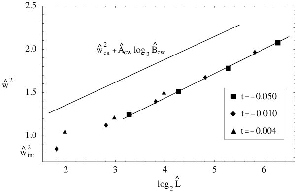
Figure 3: Total interface widths $\hat{w}^{2}$ (in temperature-independent units) of profiles for $B=L$ at the given temperatures $t$. Statistical errors are smaller than the displayed symbols. For comparison, the intrinsic width $\hat{w}^{2}_{\mathrm{int}}=\pi^{2}/12$ and the prediction $\hat{w}_{\mathrm{ca}}^{2}$ from the convolution approximation (with an offset $\hat{A}_{\mathrm{cw}}\log_{2}\hat{B}_{\mathrm{cw}}$) are shown.

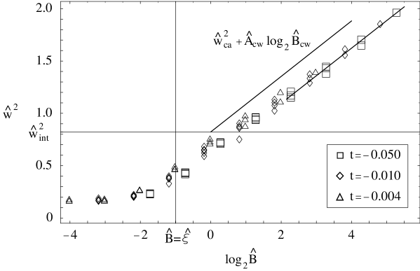
Figure 4: Interface widths $\hat{w}^{2}$ (in temperature-independent units) of profiles coarse grained on block lengths $B<L$. Symbols are as in Fig. 3. In addition, the correlation length $\hat{\xi}$ is shown.

References

- [1] B. Widom, in Phase Transitions and Critical Phenomena, Vol. 2, C. Domb and M. Green, eds. (Academic Press, 1972).
- [2] J. Rowlinson and S. Widom, Molecular theory of capillarity (Clarendon Press, 1982).
- [3] K. Binder, in Phase Transitions and Critical Phenomena, Vol. 8, C. Domb and J. Lebowitz, eds. (Academic Press, 1983).
- [4] D. Jasnow, Critical phenomena at interfaces, Rep. Prog. Phys. 47: 1059-1132 (1984).
- [5] J. van der Waals, The thermodynamic theory of capillarity under the hypothesis of a continuous variation of density, Verhandel Konink. Akad. Weten. 1 (1893). English translation: J. Rowlinson, J. Stat. Phys. 20: 97-244 (1979).
- [6] J. Cahn and J. Hillard, Free energy of a nonuniform system, J. Chem. Phys. 28: 258-267 (1958).
- [7] S. Fisk and B. Widom, Structure and free energy of the interface between fluid phases in equilibrium near the critical point, J. Chem. Phys. 50: 3219-3227 (1960).
- [8] F. Buff, R. Lovett and F. Stillinger, Interfacial density profile for fluids in the critical region, Phys. Rev. Lett. 15: 621-623 (1965).
- [9] M. Gelfand and M. Fisher, Finite-size effects in fluid interfaces. Physica A 166: 1-74 (1990).
- [10] M. Sanyal, S. Sinha, K. Huang and B. Ocko, X-ray-scattering study of capillary-wave fluctuations at a liquid surface, Phys. Rev. Lett. 66: 628-631 (1991); I. Tidswell, T. Rabedeau, P. Pershan and S. Kosowsky, Complete Wetting of a rough surface: an x-ray study, Phys. Rev. Lett. 66: 2108-2111 (1991).
- [11] M. Tolan, O. Seeck, J. Schlomka, W. Press, J. Wang, S. Sinha, Z. Li, M. Rafailovich and J. Sokolov, Evidence for capillary waves on dewetted polymer film surfaces: A combined x-ray and atomic force microscopy study, Phys. Rev. Lett. 81: 2731-2734 (1998); K. Shull, A. Mayes and T. Russell, Segment distributions in lamellar diblock copolymers, Macromolecules 26: 3929-3936 (1993); M. Sferrazza, C. Xiao, R. Jones, D. Bucknall, J. Webster and J. Penfold, Evidence for capillary waves at immiscible polymer/polymer-interfaces, Phys. Rev. Lett. 78: 3693-3696 (1997); J. Scherble, B. Stark, B. Stuhn, J. Kressler, H. Budde, S. Horing, D. Schubert, P. Simon and M. Stamm, Comparison of interfacial width of block copolymers of -poly(methyl methacrylate) with various poly(n-alkyl methacrylate)s and the respective homopolymer pairs as measured by neutron reflection, Macromolecules 32: 1859-1864 (1999).
- [12] A. Werner, F. Schmid, M. Müller and K. Binder, Anomalous size-dependence of interfacial profiles between coexisting phases of polymer mixtures in thin film geometry: A Monte-Carlo simulation, J. Chem. Phys. 107: 8175-8188 (1997); A. Werner, F. Schmid, M. Müller and K. Binder, “Intrinsic” profiles and capillary waves at homopolymer interfaces: A Monte Carlo study, Phys. Rev. E 59: 728-738 (1999).
- [13] E. Bürkner and D. Stauffer, Monte Carlo study of surface roughening in the three-dimensional Ising model, Z. Phys. B 53: 241-243 (1983).
- [14] K. Mon, D. Landau and D. Stauffer, Interface roughening in the three-dimensional Ising model, Phys. Rev. B 42: 545-547 (1990).
- [15] M. Hasenbusch and K. Pinn, Surface tension, surface stiffness, and surface width of the 3-dimensional Iisng model on a cubic lattice, Physica A 192: 342-374 (1992).
- [16] J. Weeks, Structure and thermodynamics of the liquid-vapor interface, J. Chem. Phys. 67: 3106-3121 (1977).
- [17] M. Le Bellac, Quantum and Statistical Field Theory, (Clarendon Press, 1991).
- [18] J. Küster and G. Münster, in preparation.
- [19] N. J. Günther, D. A. Nicole and D. J. Wallace, Goldstone modes in vacuum decay and first-order phase transitions, J. Phys. A 13: 1755-1767 (1980).
- [20] M. Hasenbusch and K. Pinn, The interface tension of the three-dimensional Ising model in the scaling region, Physica A 245: 366-378 (1997).
- [21] P. Hoppe and G. Münster, The interface tension of the three-dimensional Ising model in two-loop order, Phys. Lett. A 238: 265-269 (1998).
- [22] U. Wolff, Collective Monte Carlo updating for spin systems, Phys. Rev. Lett. 62: 361-364 (1989).
- [23] M. Hasenbusch, S. Meyer and M. Pütz, The roughening transition of the 3d Ising Interface: A Monte Carlo study, J. Stat. Phys. 85: 383-401 (1996).
- [24] D. Stauffer, Oil-water interfaces in the Ising model, Progr. Colloid Polym. Sci. 103: 60-66 (1997).
- [25] M. Müller, Fluktuationen kritischer Grenzflächen auf verschiedenen Größenskalen, Diploma thesis, University of Münster, Jan. 2004.
- [26] F. Schmid and K. Binder, Rough interfaces in a bcc-based binary alloy, Phys. Rev. B46: 13553-13564 (1992).
- [27] R. Guida and J. Zinn-Justin, Critical exponents of the N-vector model, J. Phys. A 31: 8103-8121 (1998).
- [28] M. Caselle, F. Gliozzi, U. Magnea and S. Vinti, Width of long colour flux tubes in lattice gauge systems, Nucl. Phys. B 460: 397-412 (1996).