Josephson current through a nanoscale magnetic quantum dot

Abstract

We present theoretical results for the equilibrium Josephson current through an Anderson dot tuned into the magnetic regime, using Hirsch-Fye Monte Carlo simulations covering the complete crossover from Kondo-dominated physics to $\pi$ junction behavior in a numerically exact way. Within the ‘magnetic’ regime, $U/\Gamma\gg 1$ and $\epsilon_{0}/\Gamma\leq 1$, the Josephson current is found to depend only on $\Delta/T_{K}$, where $\Delta$ is the BCS gap and $T_{K}$ the Kondo temperature. The junction behavior can be classified into four different quantum phases. We describe these behaviors, specify the associated three transition points, and identify a local minimum in the critical current of the junction as a function of $\Delta/T_{K}$.

Recent advances in nanoscale manipulation and fabrication call for a deeper understanding of the effect of electronic correlations. Due to the complexity of its theoretical treatment, the interplay between superconductivity and magnetism belongs to the least understood phenomena in that respect. Here we study the Josephson current $I(\phi)$ through a correlated nanoscale quantum dot contacted by $s$-wave BCS superconductors. At low enough temperatures, such a dot is generally described by the Anderson impurity model indicated in Fig. 1. We consider the regime $U/\Gamma\gg 1$ and $\epsilon_{0}/\Gamma\ll-1$, where the dot effectively has single occupancy and thus represents a spin-1/2 degree of freedom. Then a complicated interplay between this magnetic impurity and the superconductivity in the leads sets in. Some aspects of this physics were recently observed in Andreev conductance measurements for a short multi-wall nanotube buitelaar1 ; buitelaar2 . A similar setup should also allow to probe the Josephson current in the near future, where the ratio $\Delta/T_{K}$ is widely tunable via a backgate voltage.

In this paper, we provide a detailed analysis and classification of all possible phases expected in such an experiment. We find that only one ‘master’ parameter $\Delta/T_{K}$ governs this problem, where

$$T_{K}=\frac{1}{2}\sqrt{\Gamma U}\exp[\pi\epsilon_{0}(\epsilon_{0}+U)/\Gamma U]$$ (1)

is the Kondo temperature for normal leads haldane . For $\Delta/T_{K}\ll 1$, the Kondo effect survives and is only weakly affected by superconductivity, while for $\Delta/T_{K}\gg 1$, perturbation theory in $\Gamma$ yields an inverted Josephson relation $I(\phi)=-I_{c}\sin\phi$ kulik ; shiba ; glazman ; spivak , where $\phi=\pi$ represents a minimum of the junction free energy $F(\phi)$. Such a $\pi$ junction behavior was recently reported in Nb-Cu_xNi_1-x-Nb systems ryan , is related to subgap (Andreev) bound states arovas ; clerk , and implies broken time-reversal symmetry. In both limits, analytical expressions glazman are reproduced by our method below. For a magnetic impurity, the Josephson relation is generally replaced by a more complicated dependence on $\phi$. A classification into four types of junctions, labeled as $\mathrm{𝟎}$, $0^{\prime}$, $\pi^{\prime}$ and $\pi$, follows from the respective stability of the $\phi=0$ and $\phi=\pi$ configurations arovas . For a $\mathrm{𝟎}$ ($\pi$) junction, only $\phi=0\ (\phi=\pi$) is a minimum of $F(\phi)$. For the two other cases, both $\phi=0,\pi$ are local minima, and depending on whether $\phi=0\ (\phi=\pi)$ is the global minimum, one has a $0^{\prime}$ ($\pi^{\prime}$) junction. Using $I(\phi)=(2e/\hbar)dF(\phi)/d\phi$, the phase boundaries can be directly read off from the $I(\phi)$ curves. For instance, the $0^{\prime}$-$\pi^{\prime}$ transition point is determined by the condition $\int_{0}^{\pi}d\phi I(\phi)=0$.

The theoretical description of the resulting phase diagram is difficult, and despite intense efforts over the past few years arovas ; clerk ; ando ; yosh ; roz ; guinea ; mats ; kozub ; vecino ; belzig , a satisfactory physical picture has not been obtained so far. This paper provides numerically exact results for a magnetic Josephson junction from Monte Carlo (MC) simulations, using a Hirsch-Fye algorithm hirsch ; fye ; kusa adapted to this problem. We find that previous approximate theories for this problem, relying on the non-crossing approximation (NCA) for $U\to\infty$ clerk ; ando ; roz , mean-field approaches arovas ; vecino , perturbative schemes guinea ; mats ; kozub ; vecino , or the numerical renormalization group (NRG) yosh ; belzig , lead to incomplete and sometimes even qualitatively inaccurate predictions. Although the existence of the above-mentioned phases follows already from mean-field theory arovas , their respective stability and the actual phase boundaries have not been reliably established. Moreover, the critical current defined by

$$I_{c}(\Delta/T_{K})={\rm max}_{\phi}\ |I(\phi,\Delta/T_{K})|$$ (2)

has a non-monotonic behavior as a function of $\Delta/T_{K}$ which has been missed by all previous studies. The predicted minimum as well as the phase boundaries specified in Eqs. (8,9,10) below should be observable in state-of-the-art experiments.

We study the ‘canonical’ model for this problem, see Refs. glazman ; arovas ; clerk ; ando ; yosh ; roz ; guinea ; mats ; kozub ; vecino ; belzig and Fig. 1.

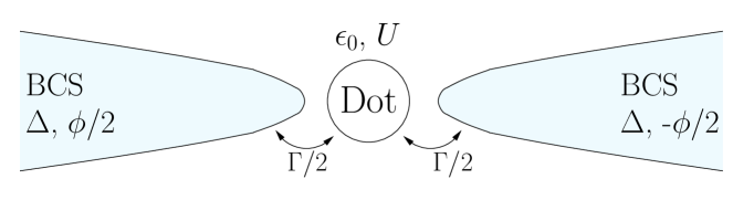
Figure 1: Schematic setup of an Anderson dot with local energy $\epsilon_{0}$ and charging energy $U>0$ coupled to BCS leads. For simplicity, we assume identical BCS gap $\Delta$ on both sides, with phase difference $\phi$ across the dot and hybridization $\Gamma$.

For a symmetric situation,

$$H = \sum_{\vec{k},p}\Bigl{[}\epsilon_{k}\sum_{\sigma}c_{\sigma,p}^{\dagger}(\vec{k})c_{\sigma,p}(\vec{k})$$

$$- \left(\Delta e^{ip\phi/2}c_{\uparrow,p}^{\dagger}(\vec{k})c_{\downarrow,p}^{\dagger}(-\vec{k})+{\rm h.c.}\right)$$

$$- \sum_{\sigma}\left(tc_{\sigma,p}(\vec{k})d^{\dagger}_{\sigma}+{\rm h.c.}\right)\Bigr{]}$$

$$+ \left(\epsilon_{0}+\frac{U}{2}\right)(n_{\uparrow}+n_{\downarrow})-\frac{U}{2}(n_{\uparrow}-n_{\downarrow})^{2},$$

where $c_{\sigma,p}(\vec{k})$ is the electron operator for lead $p=L/R=\pm$ and spin $\sigma=\uparrow,\downarrow$, with single-particle dispersion $\epsilon_{k}$. Moreover, $n_{\sigma}=d^{\dagger}_{\sigma}d_{\sigma}$ with the dot electron operator $d_{\sigma}$, and $\Gamma=2\pi\rho_{0}|t|^{2}$ for lead density of states $\rho_{0}$ and hopping matrix element $t$. In all simulations reported below, $T/\Delta=0.1$ (we put $\hbar=k_{B}=1$), which corresponds to a temperature $T\approx 100$ mK for the setup of Refs. buitelaar1 ; buitelaar2 . By comparing to analytical results for $\Delta/T_{K}\gg 1$ and $\ll 1$, this appears to be quite close to the ground-state limit.

To formulate the MC scheme, we construct the imaginary-time path integral representation under this model for the Josephson current. Discretizing imaginary time in steps of size $\delta=1/PT$ for $P$ discretization points, the last term in Eq. (Josephson current through a nanoscale magnetic quantum dot) can be decoupled by auxiliary Ising spins $s_{k}=\pm 1$ defined at times $\tau_{k}=k\delta$, where $k=1,\ldots,P$, using the discrete Hubbard-Stratonovich transformation hirsch

$$e^{(U\delta/2)(n_{\uparrow}-n_{\downarrow})^{2}(\tau_{k})}=\frac{1}{2}\sum_{s_{k}=\pm 1}e^{-\lambda s_{k}(n_{\uparrow}-n_{\downarrow})(\tau_{k})},$$ (4)

where $\lambda=\cosh^{-1}[\exp(U\delta/2)]$. All fermions characterizing the dot and the leads are then free and can be integrated out. Thereby the Josephson current is expressed in terms of a cyclic 1D Ising spin chain with non-standard long-ranged spin-spin interactions,

$$\frac{I(\phi)}{I_{0}}=\frac{\sum_{\{s\}}{\rm det}(\hat{G}^{-1}+\lambda\hat{s})\ {\rm Tr}\left\{[\hat{G}^{-1}+\lambda\hat{s}]^{-1}\hat{\Sigma}^{J}\right\}}{\sum_{\{s\}}{\rm det}(\hat{G}^{-1}+\lambda\hat{s})},$$ (5)

where $I_{0}=e\Delta/\hbar$ is the critical current in the unitary limit, $\hat{s}$ has matrix elements $\hat{s}_{ij,\mu\nu}=s_{i}\delta_{ij}\delta_{\mu\nu}$ with Nambu indices $\mu,\nu=1,2$ and time indices $i,j$, and

$$\hat{G}^{-1}_{ij} = \delta^{2}T\sum_{\omega_{n}}e^{-i\omega_{n}\delta(i-j)}\Bigl{[}-i\omega_{n}\tau_{0}+(\epsilon_{0}+U/2)\tau_{3}$$

$$- \frac{\Gamma}{\sqrt{\omega_{n}^{2}+\Delta^{2}}}\left(i\omega_{n}\tau_{0}+\Delta\cos(\phi/2)\tau_{1}\right)\Bigr{]}.$$ (6)

The Josephson self energy is

$$\hat{\Sigma}^{J}_{ij}=-(\delta T)^{2}\Gamma\sin(\phi/2)\tau_{1}\sum_{\omega_{n}}\frac{e^{-i\omega_{n}\delta(i-j)}}{\sqrt{\omega_{n}^{2}+\Delta^{2}}}.$$ (7)

All summations over fermion Matsubara frequencies $\omega_{n}=(2n+1)\pi T$ are restricted to $|\omega_{n}|<\pi/\delta$, since finite $\delta$ implies the existence of a UV cutoff. The Pauli matrices $\tau_{i}$ act in Nambu space, with $\tau_{0}={\rm diag}(1,1)$. We mention that a modified version of this approach could also access the case of unconventional superconductor leads, where additional features are expected newref ; aono .

Equation (5) allows to compute the equilibrium Josephson current for arbitrary parameters under a MC scheme. Finite-$\delta$ corrections can be eliminated by exploiting the theorem that such corrections must scale $\propto\delta^{2}$ for any Hermitian observable fye . For given physical parameters, we thus compute $I(\phi)$ for a few (small) values of $\delta$, and then perform the extrapolation $\delta\to 0$ using a linear-regression fit. The $\delta^{2}$ scaling is well obeyed for $\Delta\delta\leq 0.1$ even for $U/\Delta=20,\Gamma/\Delta=5$, leading to discretization numbers $P\approx$ 140 to 270. Then no systematic errors are present, and numerical results are exact within stochastic MC error bars. Due to the absence of particle-hole symmetry, this algorithm has a sign problem for $\Delta\neq 0$, which manifests itself in occasionally negative determinants in Eq. (5). Fortunately, this problem is very weak in our implementation, with average sign above $0.7$, and hence does not restrict the method in practice. Local flip updates of the Ising spins under the standard Metropolis algorithm were sufficient to ensure rapid equilibration and satisfactory MC acceptance rates. Under a spin flip $s_{k}\to-s_{k}$, corresponding to $\lambda\hat{s}\to\lambda\hat{s}+\hat{w}$, where $w_{ij,\mu\nu}=-2\lambda s_{k}\delta_{ik}\delta_{jk}\delta_{\mu\nu}$, the change in weight is given by the ratio $R$ of new and old determinants appearing in Eq. (5), which can be evaluated analytically. With the matrix $\hat{D}=(\hat{G}^{-1}+\lambda\hat{s})^{-1}$, we find

$$R = {\rm det}(1+\hat{D}\hat{w})=1-2\lambda s_{k}(D_{kk,11}+D_{kk,22})$$

$$+4\lambda^{2}[D_{kk,11}D_{kk,22}-D_{kk,12}D_{kk,21}].$$

Thereby the costly explicit calculation of determinants is avoided. Similarly, $\hat{D}$ can be updated without explicit matrix inversion. Typically, $10^{6}$ MC samples were accumulated to obtain each data point below. On a 2 GHz Xeon processor, our code performs at a speed of 3.7 CPU hours per $10^{5}$ samples for $P=180$.

First, the code was checked against analytical solutions available for small and large $\Delta/T_{K}$ glazman , which were accurately reproduced, see, for instance, the inset of Fig. 2 for $\Delta/T_{K}\gg 1$. Our simulations are therefore able to cover the complete crossover from Kondo-dominated physics to a $\pi$ junction. (The case $\Delta=0$ has also been studied in Refs. hirsch ; fye using this method.) Moreover, we have checked for many parameter sets that universality is fulfilled, i.e., taking different values for $\epsilon_{0}/\Delta,U/\Delta$ and/or $\Gamma/\Delta$ only affects the Josephson current via the corresponding change in $\Delta/T_{K}$. However, the two curves for $\epsilon_{0}=-U/2$ shown in the main part of Fig. 2 demonstrate that profound differences can arise even for the same $\Delta/T_{K}$, if $U/\Gamma$ is not sufficiently large. We found $U/\Gamma\geq 5$ necessary to ensure universality; otherwise charge fluctuations may alter the Josephson current even qualitatively, see Fig. 2. Universality then holds only in the true magnetic regime, and not away from it. We mention in passing that the critical current never exceeded $I_{0}$, in contrast to the prediction in Ref. mats .

We then continue by discussing the full crossover between these two limiting cases. Numerical results shown below were obtained for $5\leq U/\Gamma\leq 10$ and $0.1\leq\Delta/\Gamma\leq 10$, putting $\epsilon_{0}=-U/2$. In Figures 3 and 4, representative data for $I(\phi)$ covering this crossover are presented. Furthermore, in Fig. 5 we show the critical current (2) as a function of $\Delta/T_{K}$. For very small $\Delta/T_{K}$, the Kondo effect is dominant, and we find a $\mathrm{𝟎}$ junction with a non-sinusoidal current-phase relation close to the unitary limit, $I_{c}=I_{0}$ glazman . For larger $\Delta/T_{K}$, the relation is more sinusoidal again, and with increasing $\Delta/T_{K}$, the critical current $I_{c}$ decreases. Moreover, above a first transition point

$$(\Delta/T_{K})_{00^{\prime}}=2.8\pm 0.1,$$ (8)

for $\phi$ slightly below $\pi$, the current is negative, and under the above classification scheme, we thus enter the $0^{\prime}$ phase, see Fig. 3. By increasing $\Delta/T_{K}$ further, one eventually reaches a second transition point at

$$(\Delta/T_{K})_{0^{\prime}\pi^{\prime}}=7.2\pm 0.2.$$ (9)

At the transition point, $\int d\phi\ I(\phi)=0$. We have now reached the $\pi^{\prime}$ phase, where $\phi=\pi$ is already the global minimum, but $\phi=0$ still represents a local minimum. The true $\pi$ phase, with $\phi=\pi$ as the only minimum, is eventually reached at

$$(\Delta/T_{K})_{\pi^{\prime}\pi}=11.0\pm 0.3.$$ (10)

For $\Delta/T_{K}\gg(\Delta/T_{K})_{\pi^{\prime}\pi}$, the inverted Josephson relation $I=-I_{c}\sin\phi$ valid in the deep $\pi$ junction limit glazman is finally recovered, see Figs. 2 and 4.

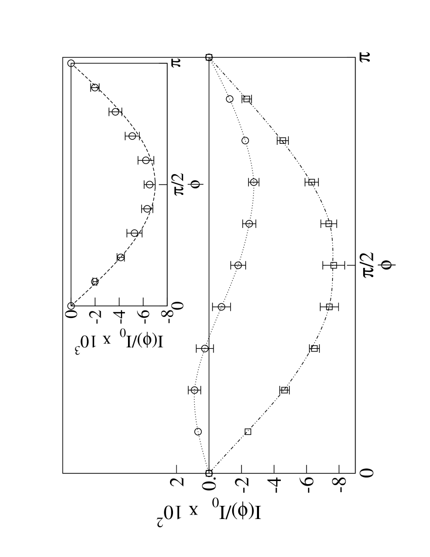
Figure 2: MC results for the Josephson current in units of $I_{0}=e\Delta/\hbar$ for two parameter sets with $\Delta/T_{K}\approx 23$. Squares are for $U/\Delta=20,\Gamma/\Delta=3.44$, and circles for $U/\Delta=4,\Gamma/\Delta=1$. Unless noted otherwise, in all figures, curves are guides to the eye only. Stochastic MC errors are always smaller than the symbol size or indicated by vertical bars. Inset: Current-phase relation in the deep $\pi$ junction regime. MC results for $\Delta/T_{K}=6.5\times 10^{4}$ coincide with the analytical result (dashed curve) glazman .

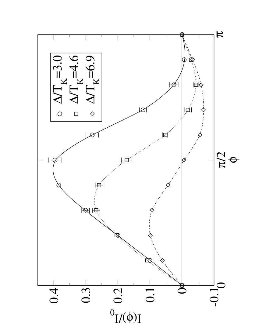
Figure 3: MC data for the current-phase relation at small-to-intermediate $\Delta/T_{K}$.

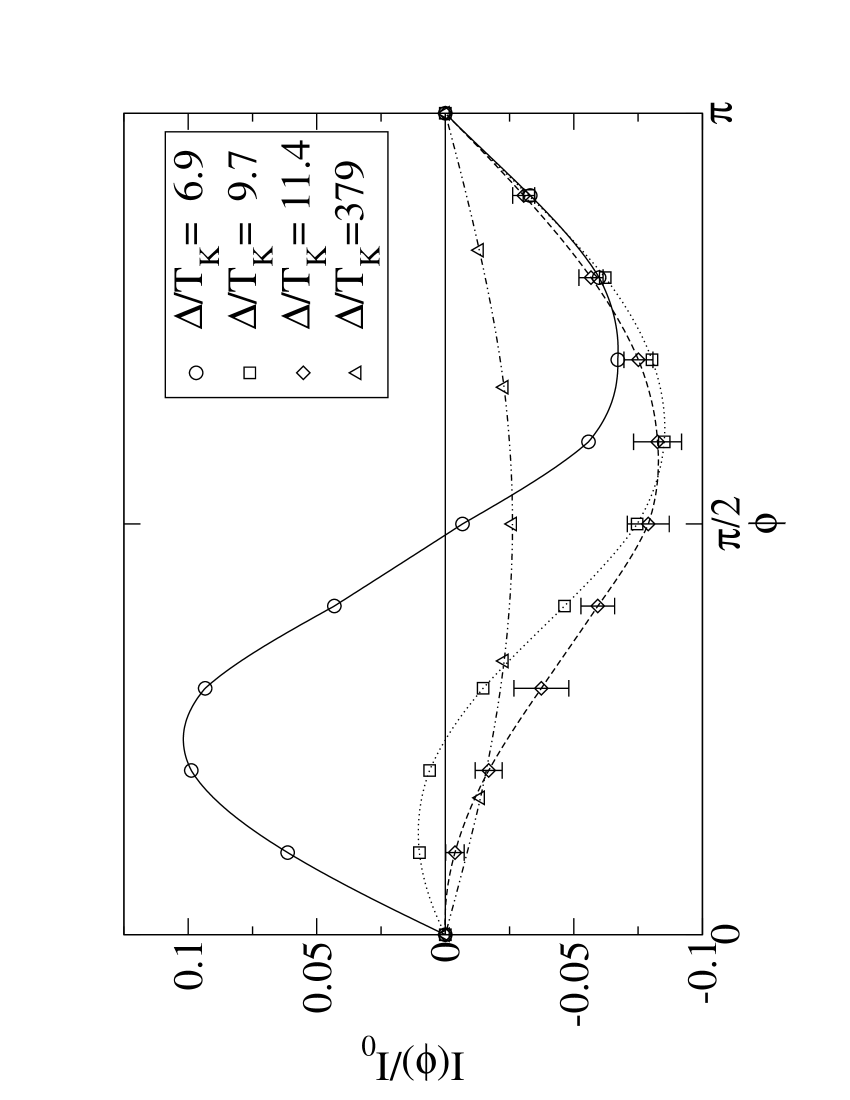
Figure 4: Same as Fig. 3 for intermediate-to-large $\Delta/T_{K}$.

The transition points reported here are at quite different locations than thought previously. For instance, NRG calculations yosh ; belzig find that the transition into the $\pi$ phase occurs at $\Delta/T_{K}\approx 2.4$, where according to our data the junction is still in the $\mathrm{𝟎}$ phase. The differences to NCA and/or mean-field results are even more drastic. According to our simulation data, the $\pi$ phase covers a much smaller region in parameter space than thought previously, while the intermediate $0^{\prime}$ and $\pi^{\prime}$ phases extend over a significant range in $\Delta/T_{K}$, and therefore should be readily observed in practice.

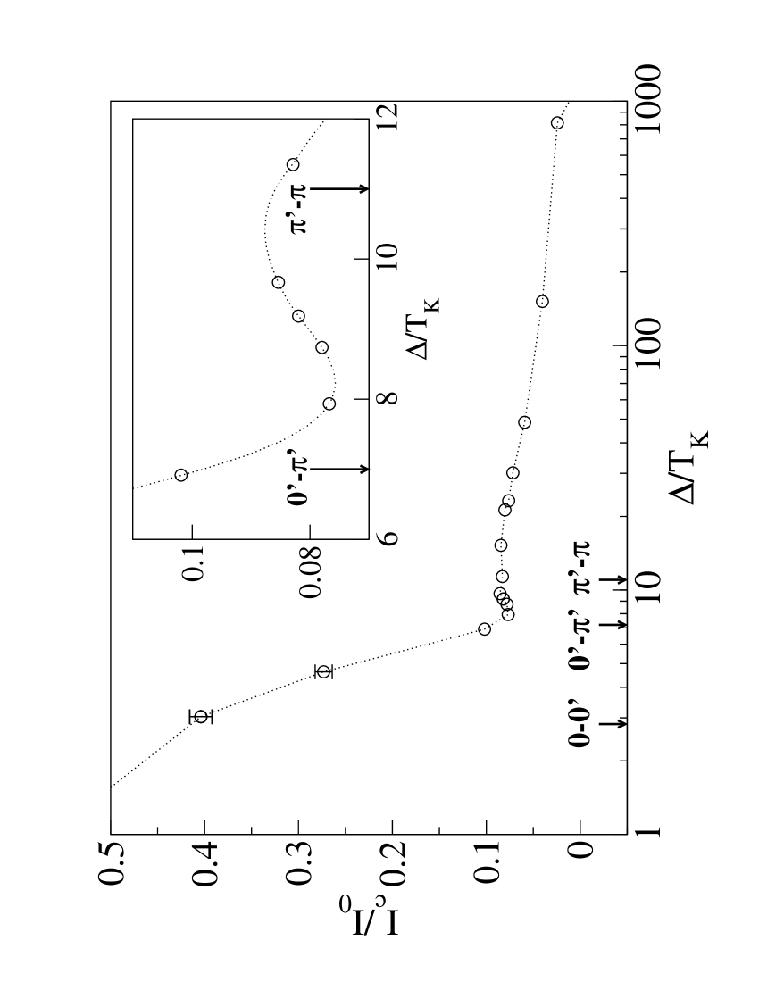
Figure 5: MC results for the critical current (2) as a function of $\Delta/T_{K}$. The arrows mark the boundaries between different phases (see text). The inset shows the region around the minimum on a magnified scale. Error bars are always smaller than symbol size.

Remarkably, the critical current shown in Fig. 5 displays non-monotonic behavior. From the analytically known limits, $I_{c}(\Delta/T_{K}\to 0)\to I_{0}$ and $I_{c}(\Delta/T_{K}\to\infty)\to 0$, a naive guess is to expect that $I_{c}(\Delta/T_{K})$ just drops monotonically with increasing $\Delta/T_{K}$. Such a behavior is in fact predicted by previous work, see, e.g., Ref. belzig . Our simulations point to a more complicated picture, where $I_{c}(\Delta/T_{K})$ is characterized by a local minimum. This minimum occurs at

$$(\Delta/T_{K})_{\rm min}=8.2\pm 0.2,$$ (11)

which is close to but above the transition point (9) for the $0^{\prime}$-$\pi^{\prime}$ transition. After reaching a local maximum slightly below the $\pi^{\prime}$-$\pi$ transition, the critical current then drops monotonically throughout the $\pi$ regime. At first sight, the local minimum in $I_{c}$ appears to resemble the experimentally observed oscillations in the critical current as a function of either temperature or length of the junction ryan . However, while those oscillations can be traced back to Andreev bound state crossings, such a simple, essentially mean-field type reasoning does not apply here, see also Ref. vecino for a closely related discussion. The appearance of a local minimum in $I_{c}$ thus indicates a subtle many-body effect.

To conclude, we have presented a numerically exact study of the Josephson current through a nanoscale dot. In the magnetic regime, $U/\Gamma\gg 1$ and $\epsilon_{0}/\Gamma\leq 1$, our results reveal a rather complex behavior that is governed by $\Delta/T_{K}$ as the only tuning parameter. These predictions should be observable in experiments on short carbon nanotube quantum dots.

We thank A. Levy Yeyati for discussions and hospitality during a visit of F. S. at the Universidad Autonoma de Madrid. This work was supported by the EU.

References

- (1) M.R. Buitelaar, T. Nussbaumer, and C. Schönenberger, Phys. Rev. Lett. 89, 256801 (2002).
- (2) M.R. Buitelaar, W. Belzig, T. Nussbaumer, B. Babic, C. Bruder, and C. Schönenberger, Phys. Rev. Lett. 91, 057005 (2003).
- (3) F.D.M. Haldane, Phys. Rev. Lett. 40, 416 (1978).
- (4) I.O. Kulik, Zh. Eksp. Teor. Fiz. 49, 585 (1965) [Sov. Phys. JETP 22, 841 (1966)].
- (5) H. Shiba and T. Soda, Prog. Theor. Phys. 41, 25 (1969).
- (6) L.I. Glazman and K.A. Matveev, Pis’ma Zh. Eksp. Teor. Fiz. 49, 570 (1989) [JETP Lett. 49, 659 (1989)].
- (7) B.I. Spivak and S.A. Kivelson, Phys. Rev. B 43, 3740 (1991).
- (8) V.V. Ryazanov, V.A. Oboznov, A. Yu. Rusanov, A.V. Veretennikov, A.A. Golubov, and J. Aarts, Phys. Rev. Lett. 86, 2427 (2001).
- (9) A.V. Rozhkov and D.P. Arovas, Phys. Rev. Lett. 82, 2788 (1999).
- (10) A.A. Clerk and V. Ambegaokar, Phys. Rev. B 61, 9109 (2000).
- (11) S. Ishizaka, J. Sone, and T. Ando, Phys. Rev. B 52, 8358 (1995).
- (12) T. Yoshioka and Y. Ohashi, J. Phys. Soc. Jpn. 69, 1812 (2000).
- (13) A.V. Rozhkov and D.P. Arovas, Phys. Rev. B 62, 6687 (2000).
- (14) A.V. Rozhkov, D.P. Arovas, and F. Guinea, Phys. Rev. B 64, 233301 (2001).
- (15) D. Matsumoto, J. Phys. Soc. Jpn. 70, 492 (2001).
- (16) V.I. Kozub, A.V. Lopatin, and V.M. Vinokur, Phys. Rev. Lett. 90, 226805 (2003).
- (17) E. Vecino, A. Martin-Rodero, and A. Levy Yeyati, Phys. Rev. B 68, 035105 (2003).
- (18) M.-S. Choi, M. Lee, K. Jang, and W. Belzig, cond-mat/0312271.
- (19) J.E. Hirsch and R.M. Fye, Phys. Rev. Lett. 56, 2521 (1986).
- (20) R.M. Fye and J.E. Hirsch, Phys. Rev. B 38, 433 (1988).
- (21) K. Kusakabe and Y. Tanaka, J. Phys. Chem. Sol. 63, 1511 (2002).
- (22) S. Kashiwaya and Y. Tanaka, Rep. Prog. Phys. 63, 1641 (2000).
- (23) T. Aono, A. Golub, and Y. Avishai, Phys. Rev. B 68, 045312 (2003).