Critical behavior of O(2)$\otimes$O($N$) symmetric models

Abstract

We investigate the controversial issue of the existence of universality classes describing critical phenomena in three-dimensional systems characterized by a matrix order parameter with symmetry O(2)$\otimes$O($N$) and symmetry-breaking pattern O(2)$\otimes$O($N$)$\rightarrow$O(2)$\otimes$O($N-2$). Physical realizations of these systems are, for example, frustrated spin models with noncollinear order.

Starting from the field-theoretical Landau-Ginzburg-Wilson Hamiltonian, we consider the massless critical theory and the minimal-subtraction scheme without $\epsilon$ expansion. The three-dimensional analysis of the corresponding five-loop series shows the existence of a stable fixed point for $N=2$ and $N=3$, confirming recent field-theoretical results based on a six-loop expansion in the alternative zero-momentum renormalization scheme defined in the massive disordered phase.

In addition, we report numerical Monte Carlo simulations of a class of three-dimensional O(2)$\otimes$O(2)-symmetric lattice models. The results provide further support to the existence of the O(2)$\otimes$O(2) universality class predicted by the field-theoretical analyses.

I Introduction

Several interesting critical transitions are effectively described by a matrix order parameter with symmetry O(2)$\otimes$O($N$) and symmetry-breaking pattern O(2)$\otimes$O($N$)$\rightarrow$O(2)$\otimes$O($N-2$). This is the case, for $N=2$ or $N=3$, of multicomponent frustrated magnetic systems with noncollinear order, in which frustration may arise either because of the special geometry of the lattice or from the competition of different kinds of interactions. Typical examples of systems of the first type are stacked triangular antiferromagnets (STA’s), in which the magnetic ions are located at the sites of a stacked triangular lattice. Frustration due to the competition of interactions is realized in helimagnets, in which a magnetic spiral is formed along a certain direction of the lattice. The nature of the magnetic transition in these materials has been the object of several studies, see, e.g., Refs. [1, 2, 3, 4, 5] for reviews. In particular, the order of the transition is still controversial, with several contradictory results both on theoretical and experimental sides.

The Landau-Ginzburg-Wilson (LGW) theory with O(2)$\otimes$O($N$) symmetry that is expected to describe these systems is given by [6]

$${\cal H}_{\rm LGW}=\int d^{d}x\Bigl{\{}{1\over 2}\sum_{a}\Bigl{[}(\partial_{\mu}\phi_{a})^{2}+r\phi_{a}^{2}\Bigr{]}+{1\over 4!}u_{0}\Bigl{(}\sum_{a}\phi_{a}^{2}\Bigr{)}^{2}+{1\over 4!}v_{0}\sum_{a,b}\Bigl{[}(\phi_{a}\cdot\phi_{b})^{2}-\phi_{a}^{2}\phi_{b}^{2}\Bigr{]}\Bigr{\}},$$ (1)

where $\phi_{a}$ ($a=1,2$) are $N$-component vectors. The symmetry-breaking pattern [7] O(2)$\otimes$O($N$)$\rightarrow$O(2)$\otimes$O($N-2$) is obtained by requiring $v_{0}>0$. Negative values of $v_{0}$ lead to a different symmetry-breaking pattern: the ground state configurations have a ferromagnetic or antiferromagnetic order and correspond to O(2)$\otimes$O($N$)$\rightarrow{\mathbb{Z}}_{2}\otimes$O($N-1$). For $v_{0}<0$ the model is also of interest; it describes magnets with sinusoidal spin structures [8, 6] and, for $N=3$, the superfluid transition of ³He [9, 10, 11]; see, e.g., Refs. [12, 3, 4, 13] for other applications. Here, we will only focus on the case $v_{0}>0$ and thus whenever we speak of an O(2)$\otimes$O($N$) universality class we refer to the case in which the symmetry-breaking pattern is O(2)$\otimes$O($N$)$\rightarrow$O(2)$\otimes$O($N-2$).

The O(2)$\otimes$O($N$) theory (1) has been much studied using field-theoretical (FT) methods. Different perturbative schemes have been exploited, such as the $\epsilon\equiv 4-d$ expansion [14] and the three-dimensional (3-$d$) massive zero-momentum (MZM) renormalization scheme [15]. A detailed discussion of the scenario emerging from the $\epsilon$ expansion is presented in Ref. [3]. Near four dimensions a stable O(2)$\otimes$O($N$) fixed point (FP) with $v_{0}>0$ is found [6, 16, 17] only for large values of $N$, $N>N_{c}=21.80-23.43\epsilon+7.09\epsilon^{2}+O(\epsilon^{3})$. Resummations of the $\epsilon$ expansion of $N_{c}$, known to $O(\epsilon^{4})$ [17], suggest [17, 18] $N_{c}\approx 6$ in three dimensions. Therefore, a smooth extrapolation of the scenario around $d=4$ to $d=3$ would indicate that a new O(2)$\otimes$O($N$) universality class does not exist for the physically interesting cases $N=2$ and 3. On the other hand, six-loop calculations in the framework of the 3-$d$ MZM scheme provide a rather robust evidence for the existence of a new stable FP for $N=2$ and $N=3$ with attraction domain in the region $v_{0}>0$ [19, 20]. This FP was found only in the analysis of high-order series, starting at four loops, while earlier lower-order calculations up to three loops [12] did not find it. According to renormalization-group (RG) theory, the stable FP of the O(2)$\otimes$O($N$) theory should describe the critical behavior of 3-$d$ systems undergoing continuous transitions characterized by the symmetry-breaking pattern O(2)$\otimes$O($N$)$\rightarrow$O(2)$\otimes$O($N-2$). The main problem of the calculations within the MZM scheme is the fact that, for $N=2$ and 3, the O(2)$\otimes$O($N$) FP is found in a region of quartic couplings in which the perturbative expansions are not Borel summable. Therefore, a Borel transformation only provides an asymptotic expansion and convergence is not guaranteed, at variance with the case of O($N$) theories in which the Borel summability of the corresponding MZM expansion provides a solid theoretical basis for the resummation methods. In the case of the O(2)$\otimes$O($N$) theory the reliability of the results concerning the new stable FP is essentially verified a posteriori from their stability with respect to the perturbative order. The MZM expansions have also been analyzed by using the pseudo-$\epsilon$ expansion method [17, 21]. No stable FP is found for $N=2$ and 3, but this is not unexpected since this resummation method can only find FPs that are already present at one loop, similarly to the $\epsilon$ expansion. We finally mention that perturbative studies of the corresponding nonlinear $\sigma$ models near two dimensions have been reported in Refs. [22, 23].

We mention that there are other physically interesting cases in which low-order $\epsilon$-expansion calculations fail to provide the correct physical picture: for example, the Ginzburg-Landau model of superconductors, in which a complex scalar field couples to a gauge field. Although $\epsilon$-expansion calculations do not find a stable FP [24], thus predicting first-order transitions, it is now well established (see, e.g., Refs. [25, 26]) that 3-$d$ systems described by the Ginzburg-Landau model can also undergo a continuous transition—this implies the presence of a stable FP in the 3-$d$ Ginzburg-Landau theory—in agreement with experiments [27].

The O(2)$\otimes$O($N$) theory has also been studied by exploiting an alternative FT method based on the analysis of the RG flow of the so-called effective average action [28, 29, 30, 31, 5]. This approach does not rely on a perturbative expansion around the Gaussian FP and it is therefore intrinsically nonperturbative. However, the practical implementation requires approximations and truncations of the average effective action. For this purpose, a derivative expansion of the effective average action is usually performed. The studies of the O(2)$\otimes$O($N$) theory reported in the literature [29, 30, 31, 5], based on the zeroth- and first-order approximations, do not find evidence of stable O(2)$\otimes$O($N$) FPs for $N=2$ and 3, in contradiction with the perturbative MZM results. This would imply that phase transitions characterized by the symmetry-breaking pattern O(2)$\otimes$O($N$)$\rightarrow$O(2)$\otimes$O($N-2$) with $N=2$ or 3 are always of first order.

The issue concerning the existence of O(2)$\otimes$O($N$) universality classes is most important to understand the physics of STA’s and of magnets with helical order, because the absence of stable O(2)$\otimes$O($N$) FPs implies that none of them can undergo a continuous transition. On the experimental side, experiments [1, 2] have apparently observed continuous transitions belonging to the O(2)$\otimes$O($N$) universality class. However, as discussed in Ref. [5], experimental results are not consistent—STA’s and helimagnets show a critical behavior with apparently different exponents—and, in some cases, do not satisfy general exponent inequalities, for instance $\gamma\leq 2\nu$ and $2\beta\geq\nu$.

The most recent Monte Carlo (MC) simulations of the antiferromagnetic XY Hamiltonian on a stacked triangular lattice have observed a first-order transition [32, 33, 34] with very small latent heat. Moreover, first-order transitions have been observed in MC investigations [35, 34] of modified lattice spin systems whose transitions are characterized by the same symmetry-breaking pattern. Therefore, MC simulations of the models considered up to now do not support the existence of an O(2)$\otimes$O(2) universality class. On the other hand, MC simulations of Heisenberg STA models, corresponding to $N=3$, give results that are substantially consistent with a continuous transition, see, e.g., Ref. [36].

We would like to stress that the existence of a universality class is not contradicted by the observation of first-order transitions in some systems sharing the same symmetry-breaking pattern. The universality class determines the critical behavior only if the system undergoes a continuous transition. Instead, first-order transitions are expected for systems that are outside the attraction domain of the stable FP. This is evident in mean-field calculations and also within the FT approach, in which some RG trajectories do not flow towards the stable FP but run away to infinity. Therefore, the above-mentioned MC results for the XY STA models are still compatible with the hypothesis of the existence of an O(2)$\otimes$O(2) universality class; XY STA models may be simply outside the attraction domain of the stable FP.

In this paper we further investigate the existence of the O(2)$\otimes$O($N$) universality class for XY ($N=2$) and Heisenberg ($N=3$) systems. First, we consider an alternative 3-$d$ perturbative approach, the so-called minimal-subtraction ($\overline{\rm MS}$) scheme without $\epsilon$ expansion [37, 38, 39], for which five-loop series have been recently computed in Ref. [17]. This scheme is strictly related to the $\epsilon$ expansion, but, unlike it, no $\epsilon$ expansion is performed and $\epsilon$ is set to the physical value $\epsilon=1$, providing a 3-$d$ scheme. It works within the massless critical theory, thus providing a nontrivial check of the results obtained within the MZM scheme, which is defined in the massive disordered phase. The analysis of the corresponding five-loop expansions shows the existence of an O(2)$\otimes$O($N$) FP for $N=2$ and 3, confirming the conclusions of the analysis of the six-loop expansions within the MZM scheme. Concerning the critical exponents, the analysis of the five-loop $\overline{\rm MS}$ series gives $\nu=0.65(6)$ and $\eta=0.09(4)$ for $N=2$, and $\nu=0.63(5)$ and $\eta=0.08(3)$ for $N=3$. These results should be compared with the estimates obtained from the six-loop MZM series, which are $\nu=0.57(3)$ and $\eta=0.09(1)$ for $N=2$, and $\nu=0.55(3)$ and $\eta=0.10(1)$ for $N=3$. It is important to note that, although the available $\overline{\rm MS}$ series have one order less, the corresponding results are expected to be more reliable than the MZM ones, because the $\overline{\rm MS}$ FPs are at the boundary of the region in which the expansions are Borel summable, and not outside it as in the MZM case. We finally mention that the $\overline{\rm MS}$ scheme without $\epsilon$ expansion allows us to obtain fixed-dimension results at any $d$. Thus, we are able to recover the results of the $\epsilon$ expansion sufficiently close to four dimensions and to obtain a full picture of the fate of the different FPs as $d$ varies from four to three dimensions.

We also address numerically the question of identifying a 3-$d$ lattice model with symmetry O(2)$\otimes$O(2) and with the expected symmetry-breaking pattern that shows a continuous transition. This would conclusively show that the O(2)$\otimes$O(2) universality class really exists. For this purpose we consider the following lattice model

$${\cal H}=-\beta\sum_{x,\mu}\left(\varphi_{x}\cdot\varphi_{x+\mu}+\psi_{x}\cdot\psi_{x+\mu}\right)+\sum_{x}\left(\varphi_{x}^{2}+\psi_{x}^{2}\right)+$$ (2)

$$\qquad\qquad+A_{4}\sum_{x}\left[(\varphi_{x}^{2}-1)^{2}+(\psi_{x}^{2}-1)^{2}\right]+2A_{22}\sum_{x}\varphi_{x}^{2}\psi_{x}^{2},$$ (3)

where $\varphi$ and $\psi$ are two-component real variables. The Hamiltonian ${\cal H}$ describes two identical two-component O(2)-symmetric lattice $\phi^{4}$ models coupled by an energy-energy term. By an appropriate change of variables, see Sec. IV, one can show that model (3) corresponds to a lattice discretization of the Hamiltonian (1) for $N=2$ with $u_{0}\sim(A_{4}+A_{22})$ and $v_{0}\sim(A_{22}-A_{4})$. When $A_{22}>A_{4}>0$ the critical behavior at the phase transition should be described by the $N=2$ Hamiltonian (1) with $v_{0}>0$. Therefore, a region of continuous transitions in the quartic parameter space with $A_{22}>A_{4}$ would imply the existence of the O(2)$\otimes$O(2) universality class. In order to investigate this point, we present MC simulations for $A_{4}=1$ and several values of $A_{22}$. The phase diagram emerging from the simulations is characterized by a line of first-order transitions extending from large values of $A_{22}$ down to a tricritical point at $A_{22}=A_{22}^{*}>A_{4}=1$, where the latent heat vanishes, and, for $1=A_{4}<A_{22}<A_{22}^{*}$, by a line of continuous transitions that should belong to the O(2)$\otimes$O(2) universality class identified by the perturbative FT approaches. The possible extension of the first-order transition line up to $A_{22}=A_{4}$, i.e. up to the 4-vector theory, is apparently incompatible with the theoretically predicted behavior of the latent heat near an O(4) tricritical point.

The paper is organized as follows. In Sec. II we present the analysis of the five-loop $\overline{\rm MS}$ expansions, providing evidence for the existence of a stable FP with attraction domain in the region $v_{0}>0$, in the two- and three-component cases. There, we also show that for $d\rightarrow 4$ the results of the $\epsilon$ expansion are recovered. In Sec. III we discuss the crossover behaviors predicted by the FT approach and their relation with those that may be observed in realistic models. In Sec. IV we report the results of the MC simulations for the model defined by Hamiltonian (3), determining its phase diagram in the region of quartic parameters $A_{22}>A_{4}=1$. We investigate the finite-size scaling (FSS) behavior using cubic lattices of size $L\leq 120$. In Sec. V we report some conclusive remarks. In App. A we provide some details on the perturbative expansions in the $\overline{\rm MS}$ scheme. In App. B we discuss some properties of O($M$)$\otimes$O($N$)-symmetric medium-range models.

II Analysis of the five-loop minimal-subtraction series

A The minimal-subtraction scheme without $\epsilon$ expansion

The FT approach is based on the Hamiltonian (1). In the $\overline{\rm MS}$ scheme one considers the massless critical theory in dimensional regularization and determines the RG functions from the divergences appearing in the perturbative expansion of the correlation functions [37]. In the standard $\epsilon$-expansion scheme [14] the FPs, i.e. the common zeroes of the $\beta$-functions, are determined perturbatively as expansions in powers of $\epsilon$, while exponents are obtained by expanding the corresponding RG functions, i.e. $\eta_{\phi,t}$ (see App. A), computed at the FP in powers of $\epsilon$. The $\overline{\rm MS}$ scheme without $\epsilon$ expansion [39] is strictly related. The RG functions $\beta_{u,v}$ and $\eta_{\phi,t}$ are the $\overline{\rm MS}$ functions. However, $\epsilon$ is no longer considered as a small quantity but it is set to its physical value, i.e. in three dimensions one simply sets $\epsilon=1$. Then, one determines the FP values $u^{*}$, $v^{*}$ from the common zeroes of the resummed $\beta$ functions. Finally, critical exponents are determined by evaluating the resummed RG functions $\eta_{\phi}$ and $\eta_{t}$ at $u^{*}$ and $v^{*}$. Notice that the FP values $u^{*}$ and $v^{*}$ are different from the FP values of the renormalized quartic couplings of the MZM renormalization scheme, since $u$ and $v$ indicate different quantities in the two schemes.

The $\overline{\rm MS}$ RG functions have been computed to five loops in Ref. [17]. In App. A we report the series for $N=2$ and $N=3$. We also consider the critical exponents associated with the chiral degrees of freedom. They can be determined from the RG dimension of the chiral operator [6]

$$C_{ckdl}(x)=\phi_{ck}(x)\phi_{dl}(x)-\phi_{cl}(x)\phi_{dk}(x).$$ (4)

We computed the $\overline{\rm MS}$ RG function $\eta_{c}(u,v)$ associated with the chiral operator $C_{ckdl}$ to five loops. The series are reported in App. A.

B The resummation

Since perturbative expansions are divergent, resummation methods must be used to obtain meaningful results. Given a generic quantity $S(u,v)$ with perturbative expansion $S(u,v)=\sum_{ij}c_{ij}u^{i}v^{j}$, we consider

$$S(xu,xv)=\sum_{k}s_{k}(u,v)x^{k},$$ (5)

which must be evaluated at $x=1$. The expansion (5) in powers of $x$ is resummed by using the conformal-mapping method [40, 41] that exploits the knowledge of the large-order behavior of the coefficients, generically given by

$$s_{k}(u,v)\sim k!\,[-A(u,v)]^{k}\,k^{b}\,\left[1+O(k^{-1})\right].$$ (6)

The quantity $A(u,v)$ is related to the singularity $t_{s}$ of the Borel transform $B(t)$ that is nearest to the origin: $t_{s}=-1/A(u,v)$. The series is Borel summable for $x>0$ if $B(t)$ does not have singularities on the positive real axis, and, in particular, if $A(u,v)>0$. Using semiclassical arguments, one can argue that [19] the expansion is Borel summable when (see App. A for the precise definition of $u$ and $v$)

$$u\geq 0,\qquad u-\frac{1}{2}v\geq 0.$$ (7)

In this region we have

$$A(u,v)=\frac{1}{2}\,{\rm Max}\left(u,u-v/2\right).$$ (8)

Under the additional assumption that the Borel-transform singularities lie only in the negative axis, the conformal-mapping method [40] turns the original expansion into a convergent one in the region (7). Outside, the expansion is not Borel summable. However, if the condition

$$u-\frac{1}{4}v>0$$ (9)

holds, then the Borel-transform singularity closest to the origin is still in the negative axis, and therefore the large-order behavior is still given by Eq. (6) with $A(u,v)$ given by Eq. (8). Thus, by using this value of $A(u,v)$ and the conformal-mapping method one still takes into account the leading large-order behavior. One may therefore hope to get an asymptotic expansion with a milder behavior, which may still provide reliable results.

We should mention that the $\overline{\rm MS}$ series are essentially four-dimensional, so that they may be affected by renormalons that make the expansion non-Borel summable for any $u$ and $v$, and are not detected by a semiclassical analysis; see, e.g., Ref. [42]. The same problem should also affect the $\overline{\rm MS}$ series of O($N$) models. However, the good agreement between the results obtained from the FT analyses [39] and those obtained by other methods indicates that renormalon effects are either very small or absent (note that, as shown in Ref. [43], this may occur in some renormalization schemes). For example, the analysis of the five-loop perturbative series [39] gives $\nu=0.629(5)$ for the Ising model and $\nu=0.667(5)$ for the XY model, that are in good agreement with the most precise estimates obtained by lattice techniques, such as $\nu=0.63012(16)$ [44] and $\nu=0.63020(12)$ [45] for the Ising model, and $\nu=0.67155(27)$ [46] for the XY universality class. On the basis of these results, we will assume renormalon effects to be negligible in the analysis of the two-variable series of the O(2)$\otimes$O($N$) theory.

C Three-dimensional analysis of the five-loop series for $N=2,3$

The RG flow of the theory is determined by the FPs. Two FPs are easily identified: the Gaussian FP, which is always unstable, and the O($2N$) FP located along the $u$ axis. The results of Ref. [48, 49] on the stability of the three-dimensional O($M$)-symmetric FP under generic perturbations can be used to prove that also the O($2N$) FP is unstable for any $N\geq 2$ [47]. Indeed, the Hamiltonian term $(\phi_{a}\cdot\phi_{b})^{2}-\phi_{a}^{2}\phi_{b}^{2}$, which acts as a perturbation at the O($2N$) FP, is a particular combination of quartic operators transforming as the spin-0 and spin-4 representations of the O($2N$) group, and any spin-4 quartic perturbation is relevant [48] at the O($M$) FP for $M\geq 3$, since its RG dimension $y_{4,4}$ is positive for $M\geq 3$. In particular, $y_{4,4}\approx 0.11$ at the O(4) FP and $y_{4,4}\approx 0.27$ at the O(6) FP [48]. Note that these values are rather small, especially in the O(4) case. The $u$-axis plays the role of a separatrix and thus the RG flow corresponding to $v_{0}>0$ cannot cross the $u$-axis. Therefore, since models with the symmetry-breaking pattern O(2)$\otimes$O($N$)$\to$O(2)$\otimes$O($N-2$) have $v_{0}>0$, the relevant FPs lie in the region $v>0$.

The analyses of the six-loop series in the MZM scheme reported in Refs. [19, 20] provided a rather robust evidence for the presence of a stable FP with attraction domain in the region $v_{0}>0$ for $N=2$ and $N=3$. In the following this result will be confirmed by the analysis of the $\overline{\rm MS}$ five-loop series. In order to investigate the RG flow in the region $v_{0}>0$, we apply essentially the same analysis method of Refs. [19, 50] (we refer to these references for details). We resum the perturbative series by means of the conformal-mapping method and, in order to understand the systematic errors, we vary two different parameters $b$ and $\alpha$ (see Ref. [50] for definitions). We also apply this method for those values of $u$ and $v$ for which the series are not Borel summable but still satisfy $u-{1\over 4}v>0$. As already discussed, the conformal-mapping method should still provide reasonable estimates since we are taking into account the leading large-order behavior.

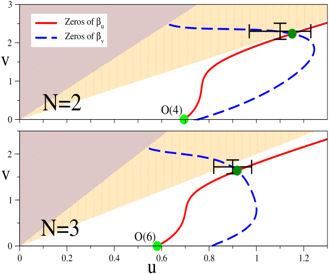
FIG. 1.: Zeroes of the $\beta$-functions in the region $v>0$ for $N=2$ and $3$ for a particular approximant, see text. The three colored regions correspond (from below) to: (1) $u-{1\over 2}v>0$ (domain in which the perturbative series are Borel summable), (2) $u-{1\over 4}v>0$ and $u-{1\over 2}v<0$ (domain in which the perturbative series are not Borel summable but one can take into account the leading large-order behavior), (3) $u-{1\over 4}v<0$. The full lines at the O(2)$\otimes$O($N$) FP show the final estimate (11) with its uncertainty.

In order to find the zeroes of the $\beta$-functions we first resummed the expansions of $B_{u}(u,v)$ and $B_{v}(u,v)$ defined in Eq. (A6). More precisely, we considered the functions $R_{u,v}(u,v,x)\equiv B_{u,v}(ux,vx)/x^{2}$. For each function $R_{u,v}$ we considered several approximants corresponding to different values of the resummation parameters $\alpha$ and $b$, see, e.g., Refs. [50, 19] for details. In Fig. 1 we show the common zeroes of the $\beta$-functions in the region $v>0$. The figure is obtained by using a single approximant, the one with $\alpha_{u}=\alpha_{v}=1$, $b_{u}=b_{v}=10$, but others give qualitatively similar results. A common zero $(u^{*},v^{*})$ with $v^{*}>0$ is clearly observed at $u^{*}\approx 1.1$, $v^{*}\approx 2.3$ for $N=2$, and at $u^{*}\approx 0.9$, $v^{*}\approx 1.7$ for $N=3$. In order to give an estimate of the FP, we considered resummations of $B_{u}(u,v)$ and $B_{v}(u,v)$ with parameters $\alpha_{u}$, $b_{u}$, $\alpha_{v}$, and $b_{v}$, assuming integer values in the range $-1\leq\alpha_{u,v}\leq 3$ and $4\leq b_{u,v}\leq 16$. Most combinations, approximately 90% for $N=2$ and 97% for $N=3$, have a common zero in the region $v>0$ (these percentages increase if we only consider approximants with $\alpha_{u}=\alpha_{v}$ and $b_{u}=b_{v}$, becoming approximately 94% for $N=2$ and 99% for $N=3$). We take the average of the results as final estimate, obtaining

$$u^{*}=1.10(13),\quad v^{*}=2.30(21)\quad {\rm for}\quad N=2,$$ (10)

$$u^{*}=0.90(8),\quad v^{*}=1.72(15)\quad {\rm for}\quad N=3.$$ (11)

The errors are related to the variation of the results with respect to changes of the resummation parameters $\alpha_{u}$, $b_{u}$, $\alpha_{v}$, and $b_{v}$ in the considered range of values, and correspond to one standard deviation. As a check, we also tried a different method. We determined optimal values of $\alpha$ and $b$ by minimizing the difference between the results of the four- and five-loop resummations of the functions $B_{u,v}$ (independently) close to the O(2)$\otimes$O($N$) FP. The results are consistent with those reported in Eq. (11). Notice that in the case $N=3$, since $v^{*}/u^{*}\approx 1.9$, the FP is substantially within the region in which the perturbative expansions should be Borel summable, while for $N=2$, since $v^{*}/u^{*}\approx 2.1$, the FP is slightly above its boundary $v/u=2$. Therefore, Borel resummations are expected to be effective. In this respect the $\overline{\rm MS}$ scheme seems to behave better than the MZM scheme, in which the FPs are in the non-Borel summable region [19], although still in the region in which the conformal-mapping resummation method should be able to take into account the leading large-order behavior. The analysis of the stability matrix shows that the FP is stable, i.e. its eigenvalues have positive real part. Most approximants give complex eigenvalues, supporting the hypothesis that the FP is a focus, as discussed in Ref. [20]. We obtain $\omega=1.0(5)\pm i0.8(5)$ for $N=2$ and $\omega=0.9(4)\pm i0.7(3)$ for $N=3$, in rough agreement with the MZM scheme results [20]. We finally mention that consistent results are obtained by resumming the series using the Padé-Borel technique, which does not exploit the knowledge of the large-order behavior of the series.

Critical exponents are obtained by evaluating the RG functions $\eta_{\phi}$ and $\eta_{t}$ or appropriate combinations at the FP. We found

$$\nu=0.65(2+4),\quad\eta=0.09(2+2),\quad\gamma=1.24(3+8),\quad\phi_{c}=1.42(6+10)$$ (12)

for $N=2$, and

$$\nu=0.63(1+4),\quad\eta=0.08(2+1),\quad\gamma=1.20(1+7),\quad\phi_{c}=1.35(2+7)$$ (13)

for $N=3$. The errors are reported as the sum of two terms, related respectively to the dependence on $b$ and $\alpha$ and to the uncertainty of the FP coordinates. For comparison we report the corresponding results obtained from the analysis of the six-loop series in the MZM scheme [19, 51]: $\nu=0.57(3)$, $\eta=0.09(1)$ and $\phi_{c}=1.43(4)$ for $N=2$, and $\nu=0.55(3)$, $\eta=0.10(1)$ and $\phi_{c}=1.27(4)$ for $N=3$. We note that the $\overline{\rm MS}$ estimates of $\nu$ and $\gamma$ are larger than those obtained in the MZM scheme, but still substantially compatible with them taking into account their relatively large errors. We stress again that this comparison represents a nontrivial consistency check since the two schemes are quite different: in the MZM scheme one works in the massive high-temperature phase, while in the $\overline{\rm MS}$ scheme one considers the massless critical theory.

Finally, we computed the RG flow, in order to determine the attraction domain of the stable FP. We refer the reader to Ref. [52] for the relevant definitions. In Fig. 2 we show the RG flow in the quartic-coupling $u,v$ plane corresponding to different values of the ratio $s\equiv v_{0}/u_{0}$ for $v_{0}>0$. All trajectories corresponding to $s\lesssim 3/2$ belong to the region $u-{1\over 2}v\gtrsim 0$, in which the resummation should be reliable, and appear to be attracted by the stable FP.

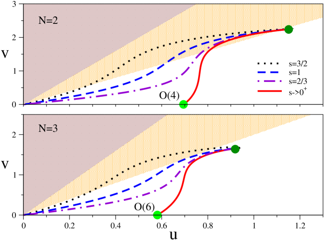
FIG. 2.: The RG flow in the quartic-coupling plane for $N=2,3$ in the $\overline{\rm MS}$ scheme for $d=3$.

D Results for generic values of $N$ and dimension $d$

The fixed-dimension $\overline{\rm MS}$ scheme allows us to obtain fixed-dimension results for any dimension $d$. Since in three dimensions and for $N=2$, 3 this scheme provides results that are substantially different from those of the strictly related $\epsilon$ expansion, it is interesting to compare the two perturbative methods for generic values of $d$ and $N$.

Using the five-loop series of the $\overline{\rm MS}$ $\beta$-functions, we investigate the presence of FPs in the region $0\leq v<4u$, where resummations seem to be under control, for generic $d$ and $N$. In any $d$, or $\epsilon\equiv 4-d$, and for sufficiently large values of $N$, we find a stable O(2)$\otimes$O($N$) FP. If we decrease $N$ at fixed $\epsilon$, for $\epsilon$ smaller than a critical value $\epsilon_{c,\rm max}$, we find a value $N_{c}(\epsilon)$ such that, for $N=N_{c}(\epsilon)$, the stable FP disappears. In Fig. 3 we plot the results for the inverse quantity $\epsilon_{c}(N)\equiv 4-d_{c}(N)$, where $d_{c}(N)$ represents the dimension below which one finds a stable FP in the region $v>0$ at fixed $N$. This quantity may be estimated by averaging the values of the largest dimension $d$ (smallest value of $\epsilon$) for which each pair of approximants of the $\beta$-functions (we use the same set as in the three-dimensional analysis reported in Sec. II C) has a stable O(2)$\otimes$O($N$) FP. The reported error corresponds to one standard deviation. Unfortunately, for $4\lesssim N\lesssim 5$ the stable FP moves outside the region $u-{1\over 4}v>0$, in which we are able to resum reliably the perturbative series (if this condition is satisfied we can take into account the leading large-order behavior). Therefore, for $N\leq 4$ we are unable to compute $\epsilon_{c}(N)$. In this case we can compute a conservative upper bound by finding the smallest value of $\epsilon$ such that at least 95% of the approximants still present a stable FP in the region $0<v<4u$. The bounds corresponding to $N=2$, 3, and 4 are represented by thick segments in Fig. 3. There, we also compare these results with the curve obtained by resumming the $O(\epsilon^{4})$ expansion [17] of $N_{c}(\epsilon)$ (we actually report the curve obtained by resumming $1/N_{c}(\epsilon)$). A nice agreement is observed for sufficiently large values of $N$, down to $N\approx 8$. For smaller values of $N$ the fixed-dimension $\overline{\rm MS}$ results differ from the $\epsilon$-expansion curve. In particular, unlike the $\epsilon$ expansion, the fixed-dimension $\overline{\rm MS}$ series provides estimate for $\epsilon_{c}(2)$ and $\epsilon_{c}(3)$ that are definitely smaller than one, leading to the bounds $\epsilon_{c}(2)<0.7$ and $\epsilon_{c}(3)<0.8$. As Fig. 3 shows, the results for $\epsilon_{c}(N)$ are nonmonotonic, with a maximum value $\epsilon_{c,{\rm max}}\approx 0.8$ for $N\approx 8$. Thus, for $\epsilon\lesssim\epsilon_{c,{\rm max}}$ there exists another limiting value of $N$, $N_{c2}(\epsilon)$, such that for $N_{c2}(\epsilon)<N<N_{c}(\epsilon)$ no stable FP exists in the region $v\geq 0$, while for $N<N_{c2}(\epsilon)$ the O(2)$\otimes$O($N$) FP is again present. Note that while for $N>N_{c}(\epsilon)$ the stable FP has real stability eigenvalues, for $N<N_{c2}(\epsilon)$ it is a stable focus, i.e., the stability eigenvalues are complex with positive real part.

The $\overline{\rm MS}$ results are qualitatively consistent with the MZM ones, although the estimate of $\epsilon_{c,\rm max}$, $\epsilon_{c,\rm max}\approx 0.8$, apparently contradicts the conclusions of Ref. [19]. Indeed, from the analysis of the MZM scheme expansions, Ref. [19] did not find a clear evidence of stable FPs for $5\lesssim N\lesssim 7$, which would imply that $\epsilon_{c,\rm max}\gtrsim 1$. This conclusion was also in contrast with the MC results of Ref. [53] that apparently found a continuous transition for $N=6$. On the basis of the present analysis we are now inclined to believe that this may be only a resummation problem, in some sense connected to the fact that in the extended space $(N,d)$, $N=6$ and $d=3$ is close to the line $d=d_{c}(N)$.

Although in the three-dimensional $\overline{\rm MS}$ calculation, $N=6$ does not represent a special point for the existence of the FP, such a value still plays a special role. In $d=3$ the FP is topologically different for small and large values of $N$ since the stability eigenvalues are real for large $N$, while for $N=2$ and $3$ they are complex. Therefore, there should be a value $N_{\rm eq}$ that separates the two behaviors. We shall show that $N_{\rm eq}\approx 6$.

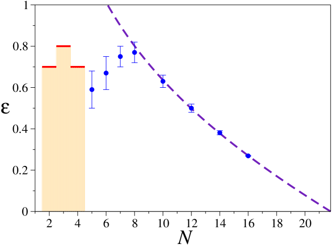
FIG. 3.: Results for $\epsilon_{c}(N)$ as obtained from the fixed-dimension $\overline{\rm MS}$ analysis and from the $\epsilon$ expansion (dashed line). The thick segments at $N=2,3,4$ represent conservative upper bounds on $\epsilon_{c}(N)$.

TABLE I.: Results obtained from the analysis of the five-loop series in the $\overline{\rm MS}$ perturbative scheme. No values of $\omega_{1,2}$ are reported for $N=6$: in this case it is not clear whether the eigenvalues of the stability matrix are complex or real.

$N$	$u^{*}$	$v^{*}$	$\omega_{1}\qquad\omega_{2}$	$\nu$	$\gamma$	$\eta$
2	1.10(13)	2.30(21)	1.0(5) $\pm i$0.8(5)	0.65(6)	1.24(11)	0.09(4)
3	0.90(8)	1.72(15)	0.9(4) $\pm i$0.7(3)	0.63(5)	1.20(8)	0.08(3)
4	0.74(3)	1.29(8)	0.7(2) $\pm i$0.4(2)	0.64(4)	1.24(6)	0.073(10)
5	0.63(3)	1.04(7)	0.7(2) $\pm i$0.3(2)	0.64(4)	1.25(6)	0.061(10)
6	0.56(4)	0.86(7)		0.66(4)	1.29(8)	0.052(14)
7	0.51(5)	0.73(5)	0.8(2)      0.5(2)	0.68(4)	1.34(9)	0.047(15)
8	0.47(4)	0.64(4)	0.8(2)      0.5(2)	0.70(5)	1.37(10)	0.042(10)
10	0.41(4)	0.51(1)	0.9(2)      0.5(2)	0.74(5)	1.46(11)	0.036(8)
16	0.300(14)	0.334(8)	0.9(2)      0.74(12)	0.82(4)	1.62(8)	0.025(4)

For large values of $N$ the stability eigenvalues are real. As $N$ decreases the difference between $\omega_{1}$ and $\omega_{2}$ decreases and for $N=N_{\rm eq}$ we have $\omega_{1}=\omega_{2}$. Then, for $N<N_{\rm eq}$ the eigenvalues become complex and the FP is a focus. As it can be seen from the results reported in Table I, $N_{\rm eq}\approx 6$. In this case, $\approx$ 50% of the approximants give real estimates for $\omega_{1}$ and $\omega_{2}$, while $\approx$ 50% give complex estimates with a small imaginary part. In all cases the real part satisfies $0.3<\hbox{{$\Re$}{\rm e}}\,\omega_{i}<0.8$.

Beside the stability eigenvalues in Table I we also report the critical exponents and the FP coordinates for several values of $N$. These results are in agreement with the MZM estimates of Ref. [20]. We also note that the $\overline{\rm MS}$ results for $N=6$ are in substantial agreemeent with the MC results of Ref. [53], $\nu=0.700(11)$ and $\gamma=1.383(36)$, and with the nonperturbative RG results of Ref. [5], $\nu\approx 0.707$ and $\gamma\approx 1.377$.

III Crossover behavior

A Effective exponents

The perturbative analysis presented in Sec. II as well as the analyses in the MZM scheme of Ref. [19] predict the presence of a stable FP for the physically interesting cases $N=2$ and $N=3$. However, this FP has a quite unusual feature: the stability eigenvalues are apparenly complex with positive real part [19, 20]. In this Section we wish to understand the consequences on experimental and numerical determinations of the critical exponents and, in general, of RG-invariant quantities.

The presence of complex stability eigenvalues changes the approach to criticality. If ${\cal O}$ is a generic critical quantity we expect close to the critical point

$${\cal O}\approx C\xi^{\sigma}\left[1+a\xi^{-\omega_{R}}\cos(\omega_{I}\log\xi+b)\right],$$ (14)

where $\xi$ is the correlation length and the stability eigenvalues are written as $\omega_{R}\pm i\omega_{I}$. Scaling corrections oscillate and the approach to the asymptotic behavior is nonmonotonic.

In order to characterize the behavior of critical quantities outside the critical point, it is useful to introduce effective exponents. From the susceptibility $\chi$ and the correlation length $\xi$ one can define the effective exponents

$$\nu_{\rm eff}(t)\equiv-{\partial{\rm ln}\xi\over\partial{\rm ln}t},\qquad\gamma_{\rm eff}(t)\equiv-{\partial{\rm ln}\chi\over\partial{\rm ln}t},\qquad\eta_{\rm eff}(t)\equiv 2-{\partial{\rm ln}\chi\over\partial{\rm ln}\xi},$$ (15)

where $t\equiv(T-T_{c})/T_{c}$ is the reduced temperature. One can easily check that $\eta_{\rm eff}=2-\gamma_{\rm eff}/\nu_{\rm eff}$. The effective exponents are not universal and depend on the specific model. Nonetheless, it is usually assumed (but there are notable exceptions; for instance, the 3-$d$ Ising model and the corresponding scalar $\phi^{4}$ theory behave differently near the critical point [54, 55, 56]) that the qualitative features are similar in all models belonging to the same universality class. For this reason, in the following we shall compute the effective exponents in the FT model. We shall present numerical results for $N=2$, in order to be able to compare them with the MC results of Sec. IV. For $N=3$ effective exponents are qualitatively similar.

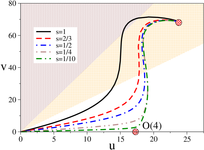
FIG. 4.: RG flow in the MZM scheme for several values of $s$ and $N=2$. The O(2)$\otimes$O(2) FP corresponds to $u^{*}=23.9(1.3)$, $v^{*}=68.7(2.5)$ (Ref. [19]).

We shall consider the MZM scheme since all necessary formulas have already been presented in Ref. [52], although the same analysis could have been done in the $\overline{\rm MS}$ scheme by generalizing to the present case the results of Ref. [57]. If $u$ and $v$ are the zero-momentum renormalized couplings normalized so that $u\approx u_{0}/m$ and $v\approx v_{0}/m$ at tree level [58], RG trajectories are determined by solving the differential equations

$$-\lambda{du\over d\lambda}=\beta_{u}(u(\lambda),v(\lambda)),$$ (16)

$$-\lambda{dv\over d\lambda}=\beta_{v}(u(\lambda),v(\lambda)),$$ (17)

where $\lambda\in[0,\infty)$, with the initial conditions

$$u(0)=v(0)=0,$$ (18)

$$\left.{du\over d\lambda}\right|_{\lambda=0}=1,\qquad\left.{dv\over d\lambda}\right|_{\lambda=0}=s,$$ (19)

where $s\equiv{v_{0}/u_{0}}$ parametrizes the different models. The results of Ref. [52] allow us to derive general scaling formulas for the rescaled $\widetilde{\chi}\equiv\chi u_{0}^{2}$ and $\widetilde{\xi}\equiv\xi u_{0}$, where $\chi$ and $\xi$ are respectively the susceptibility and the second-moment correlation length. In particular, if $\tau\equiv r-r_{c}$ is the reduced temperature and $\widetilde{\tau}\equiv\tau/u_{0}^{2}$, we have

$$\widetilde{\chi}=F_{\chi}(\widetilde{\tau},s),\qquad\qquad\widetilde{\xi}=F_{\xi}(\widetilde{\tau},s).$$ (20)

The functions $F_{\chi}$ and $F_{\xi}$ can be expressed in terms of RG functions—in the present case they are known to six loops—and can be computed rather accurately, as we shall show below.

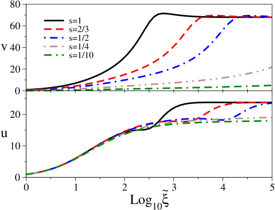
FIG. 5.: The four-point couplings $u$ and $v$ as a function of $\widetilde{\xi}$ for several values of $s$ and $N=2$. For $\widetilde{\xi}\to\infty$, $u$ and $v$ converge to $u^{*}=23.9(1.3)$ and $v^{*}=68.7(2.5)$ (Ref. [19]).

In Fig. 4 we show the RG trajectories for several values of $s$ with $0<s\leq 1$ [59]. For larger values of $s$ trajectories run in the region $u-{1\over 4}v<0$, where we are not able to resum the perturbative series. Correspondingly, in Fig. 5 we report the behavior of the four-point couplings $u$ and $v$ as a function of $\widetilde{\xi}$. The corresponding FP values [19, 58] are $u^{*}=23.9(1.3)$ and $v^{*}=68.7(2.5)$. Considering first $v(\widetilde{\xi})$, it is interesting to observe that oscillations are significant only for $s\approx 1$. For smaller values of $s$, $v(\widetilde{\xi})$ increases essentially monotonically with $\widetilde{\xi}$. More peculiar is the behavior of $u(\widetilde{\xi})$. Indeed, for all $s\lesssim 2/3$, $u$ flattens first at a value around 18 and then suddenly increases towards the asymptotic value. This is due to the presence of the unstable O(4) FP that gives rise to strong crossover effects, even when $s$ is as large as 2/3. Indeed, the plateau observed in $u$ corresponds to the FP value of $u$ in the O(4) theory [60], $u^{*}_{O(4)}\approx 17.4$. Thus, unless $s\gtrsim 1$, the flow first feels the presence of the O(4) FP, so that $u\approx u^{*}_{O(4)}$ and then goes towards the O(2)$\otimes$O(2) FP. In Fig. 6 we also show the ratio $v/u$. Note that for small $s$ such a ratio is very small, while for $s\gtrsim 1/2$ the behavior is nonmonotonic with a pronounced peak.

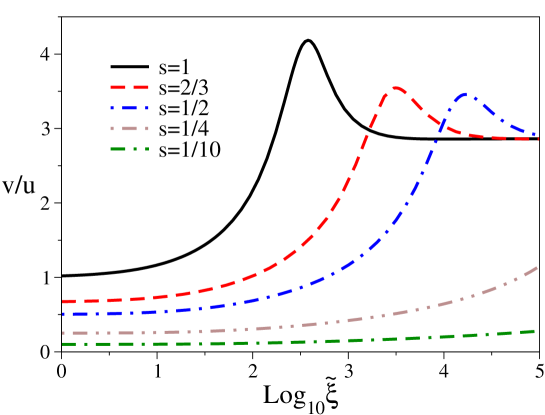
FIG. 6.: The ratio $v/u$ of the four-point couplings $u$ and $v$ as a function of $\widetilde{\xi}$ for several values of $s$ and $N=2$. Asymptotically, the ratio converges to $v^{*}/u^{*}=2.9(2)$ (Ref. [19]).

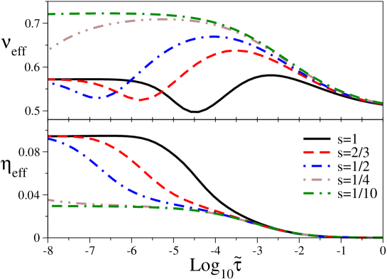
FIG. 7.: Effective exponents as a function of the rescaled reduced temperature $\widetilde{\tau}$ for several values of $s$ and $N=2$.

Finally, we determine the effective exponents. In Fig. 7 we report the effective exponents $\nu_{\rm eff}$ and $\eta_{\rm eff}$ as a function of the rescaled reduced temperature $\tilde{\tau}$. The exponent $\nu_{\rm eff}$ shows quite large oscillations, especially for small $s$. They are not only due to the complex stability eigenvalues but also to crossover effects related to the presence of the O(4) FP. As we already remarked above, for small $s$ the trajectories are close to the O(4) FP and thus $\nu_{\rm eff}$ is close to $\nu_{O(4)}$ (the best available estimate is $\nu_{O(4)}=0.749(2)$, Ref. [61]). For instance, for $s=1/4$ (resp. $s=1/2$) the maximum value of $\nu_{\rm eff}$ is 0.71 (resp. 0.67). For $s$ close to 1, crossover effects are less relevant and $\nu_{\rm eff}$ does not increase much. However, in this case there is a large downward oscillation. The exponent $\nu_{\rm eff}$ decreases below the asymptotic value and it may be even less than 0.5: for $s=1$ the minimum value of $\nu_{\rm eff}$ is 0.49 and it is expected to further decrease if $s$ increases. These oscillations show how difficult is the determination of the critical exponents: extrapolations may provide completely incorrect estimates. The effective exponent $\gamma_{\rm eff}$ has a behavior similar to that of $\nu_{\rm eff}$. On the other hand, $\eta_{\rm eff}$ shows an approximately monotonic behavior without detectable oscillations, although the crossover effects due to the presence of the O(4) FP ($\eta_{O(4)}=0.0365(10)$, Ref. [61]) are clearly visible for $s\lesssim 1/4$.

B Crossover behavior in lattice systems

In Sec. III A we computed the FT crossover curves. It is of course of interest to relate them to the results obtained in lattice models and in experimental systems. Strictly speaking, the mapping cannot go beyond the leading correction term appearing in Eq. (14) (see the discussion in Sec. IV.A of Ref. [52]). In some cases even the leading critical behavior cannot be reproduced [54, 55, 56]: this happens in the nearest-neighbor Ising model and in the lattice self-avoiding walk. However, there are limiting cases in which the FT results exactly describe the lattice model: this is the case of the critical crossover limit in weakly coupled lattice models and in medium-range models [62, 63, 64]. Consider, for instance, a $d$-dimensional hypercubic lattice and the lattice discretization of the FT Hamiltonian (1),

$${\cal H}=-{\beta\over 2}\sum_{x,y}J(x-y)\sum_{a}\varphi_{x,a}\cdot\varphi_{y,a}+\sum_{x}V(\varphi_{x}),$$ (21)

where the sums over $x$ and $y$ are extended over all lattice points, $J(x)$ is a generic short-range coupling, and

$$V(\varphi)=r\sum_{a}\varphi_{a}^{2}+{U_{0}\over 4!}(\sum_{a}\varphi_{a}^{2})^{2}+{V_{0}\over 4!}\sum_{ab}\left[(\varphi_{a}\cdot\varphi_{b})^{2}-\varphi_{a}^{2}\varphi_{b}^{2}\right].$$ (22)

The parameter $r$ is irrelevant and can be made equal to $\pm 1$ by changing the normalization of the fields.

The first interesting case corresponds to weakly coupled theories in which $r>0$ and $U_{0},V_{0}\to 0$. Let $\beta_{c}(U_{0},V_{0})$ be the critical point for given $U_{0}$ and $V_{0}$ and let $t$ be the reduced temperature. Then, consider the limit $t\to 0$, $U_{0},V_{0}\to 0$ keeping fixed $s_{L}\equiv V_{0}/U_{0}$ and $\widetilde{t}\equiv t/U_{0}^{2/(4-d)}$. In this limit

$$\chi(\beta,U_{0},V_{0})U_{0}^{2}\to\mu_{\chi}F_{\chi}(a\widetilde{t},s_{L}),$$ (23)

$$\xi(\beta,U_{0},V_{0})U_{0}\to\mu_{\xi}F_{\xi}(a\widetilde{t},s_{L}),$$ (24)

where $F_{\chi}(t,s)$ and $F_{\xi}(t,s)$ are exactly the FT functions defined in Eq. (20). The constants $\mu_{\chi}$, $\mu_{\xi}$, and $a$ can be easily computed by comparing the perturbative expansions (at one loop) for the continuum and the lattice model. The additive mass renormalization—it requires a nonperturbative matching, see Ref. [63]—also fixes the first terms of the expansion of $\beta_{c}(U_{0},V_{0})$ in powers of $U_{0}$ and $V_{0}$.

The second interesting case corresponds to medium-range models. In this case we assume that the coupling $J(x)$ depends on a parameter $\rho$. For instance, one may take

$$J_{\rho}(x)=\cases{1&$\qquad$ if $|x|\leq\rho$,\cr 0&$\qquad$ otherwise.}$$ (25)

This specific form is not necessary for the discussion that will be presented below, and indeed one can consider more general families of couplings, as discussed in Sec. 3 of Ref. [63]. The relevant property is that $J_{\rho}(x)$ couples all lattice points for $\rho\to\infty$, i.e., that for $\rho\to\infty$ one recovers a mean-field theory. The interaction range is characterized by $R$ defined by

$$R^{2}={1\over 2d}{\sum_{x}x^{2}J_{\rho}(x)\over\sum_{x}J_{\rho}(x)}.$$ (26)

These models are called medium-range models and admit an interesting scaling limit called critical crossover limit [62, 64]. If $\beta_{c}(R)$ is the critical temperature as a function of $R$ (here $U_{0}$ and $V_{0}$ are fixed and do not play any role in the limit), then for $R\to\infty$, $t\equiv(\beta_{c}(R)-\beta)/\beta_{c}(R)\to 0$ at fixed $\widetilde{t}\equiv R^{2d/(4-d)}t$, critical quantities show a scaling behavior. For instance, the susceptibility $\chi(\beta,R)$ and the correlation length $\xi(\beta,R)$ scale as

$$\widetilde{\chi} \equiv \chi(\beta,R)R^{-2d/(4-d)}\approx f_{\chi}(\widetilde{t}),$$ (27)

$$\widetilde{\xi} \equiv \xi(\beta,R)R^{-4/(4-d)}\approx f_{\xi}(\widetilde{t}).$$ (28)

The functions $f_{\chi}(\widetilde{t})$ and $f_{\xi}(\widetilde{t})$ are directly related to the crossover functions $F_{\chi}(\widetilde{\tau},s)$ and $F_{\xi}(\widetilde{\tau},s)$ computed in field theory, cf. Eq. (20). Indeed,

$$f_{\chi}(\widetilde{t}) = \mu_{\chi}F_{\chi}(a\widetilde{t},s),$$ (29)

$$f_{\xi}(\widetilde{t}) = \mu_{\xi}F_{\xi}(a\widetilde{t},s),$$ (30)

where $\mu_{\chi}$, $\mu_{\xi}$, $a$, and $s$ are nonuniversal constants that depend on the model [63, 64]. Therefore, the FT crossover functions are expected to describe accurately the crossover behavior for large $R$: in practice, numerical simulations show that for $\rho\approx 3$ one already obtains a good agreement. All constants appearing in Eq. (30) can be exactly computed by performing a one-loop calculation. The relevant formulae are reported in App. B.

IV Numerical results from Monte Carlo simulations

A The lattice model

In order to investigate the existence of the O(2)$\otimes$O(2) universality class by numerical MC simulations, we considered a simple cubic lattice $L^{3}$ and the following Hamiltonian:

$${\cal H}=-\beta\sum_{x,\mu}\left(\varphi_{x}\cdot\varphi_{x+\mu}+\psi_{x}\cdot\psi_{x+\mu}\right)+\sum_{x}\left(\varphi_{x}^{2}+\psi_{x}^{2}\right)+$$ (31)

$$\qquad\qquad+A_{4}\sum_{x}\left[(\varphi_{x}^{2}-1)^{2}+(\psi_{x}^{2}-1)^{2}\right]+2A_{22}\sum_{x}\varphi_{x}^{2}\psi_{x}^{2},$$ (32)

where $\varphi$ and $\psi$ are two-component real variables. The Hamiltonian ${\cal H}$ describes two identical two-component lattice $\phi^{4}$ models coupled by an energy-energy term. Note that if $A_{22}=A_{4}$ the symmetry is enlarged to O(4) and we have the standard four-component lattice $\phi^{4}$ model. By applying the trasformation

$$\phi_{11}={\varphi_{1}-\psi_{2}\over\sqrt{2}},\quad\phi_{12}=-{\varphi_{2}-\psi_{1}\over\sqrt{2}},\quad\phi_{21}={\varphi_{2}+\psi_{1}\over\sqrt{2}},\quad\phi_{22}={\varphi_{1}+\psi_{2}\over\sqrt{2}},$$ (33)

one can easily see that model (31) corresponds to the Hamiltonian (21) with nearest-neighbor coupling $J$ and potential (22) with

$$U_{0} = 12(A_{22}+A_{4}),$$ (34)

$$V_{0} = 24(A_{22}-A_{4}),$$ (35)

$$r = 1-2A_{4}.$$ (36)

Therefore, model (31) is a lattice discretization of the O(2)$\otimes$O(2) Hamiltonian (1). According to the FT results presented in Sec. II, continuous transitions in models with $A_{22}>A_{4}$ should be controlled by the O(2)$\otimes$O(2) FP. For $A_{22}=A_{4}$ the symmetry is enlarged to O(4) and the transition is controlled by the O(4) FP. If $A_{22}<A_{4}$ continuous transitions should belong to the XY universality class, because the O(2)$\otimes$O(2) theory has a stable XY FP with attraction domain in the region $v_{0}<0$, see, e.g., Ref. [4].

B Monte Carlo simulations

We present the results of MC simulations for several values of the quartic Hamiltonian parameters. We set $A_{4}=1$ and vary $A_{22}$, considering $A_{22}=3$, 11/4, 5/2, 9/4, 2, 5/3, and 7/5. If we define

$$s_{L}\equiv{V_{0}\over U_{0}}=2{A_{22}-A_{4}\over A_{22}+A_{4}},$$ (37)

they correspond to $s_{L}=1$, 14/15, 6/7, 10/13, 2/3, 1/2, and 1/3 respectively. Note that for $A_{22}>A_{4}>0$ we have $0<s_{L}<2$.

We simulate model (31) by using two different types of local moves: (1) a Metropolis update in which $\varphi_{x}$ and $\psi_{x}$ are both varied by adding a random term to each component in such a way to obtain a 50% acceptance; (2) an O(4) update [65] in which $\varphi_{x}$ and $\psi_{x}$ are both changed keeping fixed the O(4)-symmetric part of the Hamiltonian, while the O(4)-breaking term $2(A_{22}-A_{4})\sum_{x}\varphi_{x}^{2}\psi_{x}^{2}$ is taken into account by performing a standard Metropolis acceptance test (the acceptance of this move is rather large, varying from approximately 78% for $A_{22}=3$ to 94% for $A_{22}=7/5$). In the simulations we use a mixed algorithm in which we performed an O(4) sweep and a standard Metropolis sweep with probability 1/4 and 3/4 respectively. A rough investigation of the autocorrelation times shows that this is an optimal combination. The mixed algorithm is substantially faster (for $s_{L}=1/3$ the autocorrelation time of the magnetic susceptibility $\chi$ decreases by approximately a factor of 10) than the algorithm in which only the Metropolis update is used.

We perform a FSS study using lattices with $16\leq L\leq 120$ for values of $\beta$ close to $\beta_{c}$. The integrated autocorrelation time $\tau_{\chi}$ of the magnetic susceptibility (estimated by using the blocking method) increases approximately as $\tau_{\chi}\approx cL^{2}$ at $\beta_{c}$ with $c\approx 0.2$ for $A_{22}=7/5$ and $c\approx 0.5$ for $A_{22}=5/3$, where the time unit is an update of all spin variables. For larger values of $A_{22}$ the transition becomes of first order and the dynamics becomes very slow as $L$ increases. The large autocorrelation time, i.e. the difficulty of the updating algorithm to provide independent configurations, represents the main limitation to the study of the critical behavior at $\beta_{c}$ and for large volumes. For each value of $\beta$ we typically performed runs of a few million iterations for the smallest values of $L$, and of 20-40 million iterations for the largest lattice sizes. The total CPU time was approximately 5 CPU years of a single 64-bit Opteron 246 (2Ghz) processor.

C Definitions and notations

In order to investigate the phase diagram, it is useful to study the FSS of quantities related to the energy

$$E\equiv{1\over V}\langle{\cal H}\rangle$$ (38)

($V\equiv L^{3}$ is the volume), such as the specific heat

$$\quad C\equiv{1\over V}\left(\langle{\cal H}^{2}\rangle-\langle{\cal H}\rangle^{2}\right),$$ (39)

and the energy cumulant [66]

$$B_{E}\equiv 1-{\langle{\cal H}^{4}\rangle\over 3\langle{\cal H}^{2}\rangle^{2}}.$$ (40)

We also define a quantity $M$ related to the magnetization:

$$M\equiv\langle\;\sqrt{\mu^{2}_{\varphi}+\mu^{2}_{\psi}}\;\rangle,$$ (41)

where

$$\vec{\mu}_{\varphi}\equiv{1\over V}\sum_{x}\vec{\varphi}_{x},\qquad\vec{\mu}_{\psi}\equiv{1\over V}\sum_{x}\vec{\psi}_{x}.$$ (42)

The two-point correlation function $G(x)$ is defined as

$$G(x)\equiv\langle\varphi_{0}\cdot\varphi_{x}\;+\;\psi_{0}\cdot\psi_{x}\rangle.$$ (43)

The corresponding susceptibility $\chi$ and second-moment correlation length $\xi$ are given by

$$\chi\equiv\sum_{x}G(x),\qquad\qquad\xi^{2}\equiv{1\over 4\sin^{2}(q_{\rm min}/2)}{\widetilde{G}(0)-\widetilde{G}(q)\over\widetilde{G}(q)},$$ (44)

where $\widetilde{G}(q)$ is the Fourier transform of $G(x)$, $q=(q_{\rm min},0,0)$, and $q_{\rm min}=2\pi/L$. The finite-volume definition of $\xi$ is not unique. The definition used here has the advantage of a fast convergence to the infinite-volume limit [67].

In our FSS study we shall consider three RG-invariant ratios [68]

$$l_{\xi} \equiv {\xi/L},$$ (45)

$$B_{1} \equiv {\langle(\mu_{\varphi}^{2}+\mu_{\psi}^{2})^{2}\rangle\over\langle\mu_{\varphi}^{2}+\mu_{\psi}^{2}\rangle^{2}},$$ (46)

$$B_{2} \equiv {\langle\mu_{\varphi}^{2}\mu_{\psi}^{2}-(\mu_{\varphi}\cdot\mu_{\psi})^{2}\rangle\over\langle\mu_{\varphi}^{2}+\mu_{\psi}^{2}\rangle^{2}}.$$ (47)

Note that $B_{1}$ (resp. $B_{2}$) is equal to 3/2 (resp. 1/8) at $\beta=0$ and to 1 (resp. 0) at $\beta=\infty$.

D First-order transitions: summary of theoretical results

In the case of a first-order transition the probability distributions of the energy and of the magnetization are expected to show a double peak for large values of $L$. Therefore, as a first indication, one usually looks for a double peak in the distribution of the energy and of the magnetization. However, as discussed in the literature, see, e.g., Refs. [69, 70] and references therein, the observation of a double peak in the distribution of the energy for a few finite values of $L$ is not sufficient to conclude that the transition is a first-order one. For instance, in the two-dimensional Potts model with $q=3$ and $q=4$[71, 72], double-peak distributions are observed for relatively large lattice sizes even if the transition is known to be continuous. In order to identify definitely a first-order transition, it is necessary to perform a more careful analysis of the large-$L$ scaling properties of the distributions or, equivalently, of the specific heat, the energy cumulant, and the Binder cumulants, see, e.g., Refs. [66, 73, 74].

The difference of the two maximum values $E_{+}$ and $E_{-}$ of the energy-density distribution gives the latent heat. Alternative estimates of the latent heat can be obtained from the lattice-size scaling of the specific heat $C$ and of the energy cumulant $B_{E}$. According to the phenomenological theory [66] of first-order transitions based on the two-Gaussian Ansatz, for a lattice of size $L$ there exists a value $\beta_{\rm max}$ of $\beta$ where $C$ has a maximum, $C_{\rm max}$, and

$$\beta_{\rm max}-\beta_{c}=O(1/V),\qquad C_{\rm max}=V\left[{1\over 4}\Delta_{h}^{2}+O(1/V)\right],$$ (48)

where $\Delta_{h}$ is the (rescaled) latent heat

$$\Delta_{h}\equiv E_{+}-E_{-}.$$ (49)

Note that, since the temperature parameter $\beta$ is included in the Hamiltonian (31), $\Delta_{h}$ should be identified with the dimensionless ratio between the latent heat and the critical temperature. We recall that in the case of a continuous transition one expects

$$\beta_{\rm max}-\beta_{c}\approx aL^{-1/\nu},\qquad C_{\rm max}\approx bL^{\alpha/\nu}+c.$$ (50)

The energy cumulant $B_{E}$ can also be used to identify first-order transitions. Indeed, a careful analysis [66] shows that there is a value $\beta_{\rm min}$ where $B_{E}$ has a minimum, $B_{E,{\rm min}}$, and which is related to the latent heat. The phenomenological theory gives [75]

$$\beta_{\rm min}-\beta_{c}=O(1/V),\qquad B_{E,{\rm min}}={2\over 3}\left[1-{1\over 2}\Delta^{2}-{1\over 8}\Delta^{4}\right]+O(1/V),$$ (51)

where

$$\Delta\equiv{E_{+}-E_{-}\over\sqrt{E_{+}E_{-}}}.$$ (52)

In continuous transitions $\Delta=0$—there is only one peak in the energy distribution—and the infinite-volume limit of $B_{E,{\rm min}}$ is trivial: $\lim_{L\rightarrow\infty}B_{E,{\rm min}}=2/3$.

As discussed in Ref. [73], the distribution of the order parameter is also expected to show two peaks at $M_{+}$ and $M_{-}$, $M_{-}<M_{+}$, with $M_{-}\to 0$ as $L\to\infty$ since in the high-temperature phase there is no spontaneous magnetization. The phenomenological theory predicts that the Binder parameter can still be used to identify the critical point [the analysis shows that $\beta_{\rm cross}(L_{1},L_{2})-\beta_{c}\sim\min(L_{1},L_{2})^{-2d}$, where $\beta_{\rm cross}(L_{1},L_{2})$ is the value of $\beta$ at which $B_{1}(L_{1})=B_{1}(L_{2})$]. Moreover, it predicts

$${dB_{1}/d\beta}|_{\beta=\beta_{c}}\approx cL^{d},$$ (53)

for sufficiently large lattice sizes, where $d$ is the space dimension. More generally, close to $\beta_{c}$ the phenomenological theory predicts [73, 74]

$$B_{1}(\beta,L)\approx f[(\beta-\beta_{c})L^{d}].$$ (54)

Such a relation is valid only sufficiently close to $\beta_{c}$ since the scaling function $f(x)$ diverges for $x=x_{\rm peak}$ where $x_{\rm peak}$ is related to the position of the peak present in $B_{1}$ for $L\to\infty$. Ref. [73] indeed shows that $B_{1}(\beta,L)$ at fixed $L$ has a maximum $B_{1,\rm max}(L)$ at $\beta=\beta_{\rm peak}(L)<\beta_{c}$ with

$$B_{1,\rm max}\sim L^{d},\qquad\qquad\beta_{\rm peak}-\beta_{c}\approx c_{p}L^{-d}.$$ (55)

Thus, for $(\beta-\beta_{c})L^{d}$ close to $(\beta_{\rm peak}-\beta_{c})L^{d}=x_{\rm peak}=c_{p}$ the scaling behavior (54) breaks down [$f(x_{\rm peak})$ diverges] and subleading terms of order $L^{-d}$ must be included. In the region in which Eq. (54) holds, we have ${dB_{1}/d\beta}\approx L^{d}f^{\prime}[(\beta-\beta_{c})L^{d}]$. By using Eq. (54) we can express $(\beta-\beta_{c})L^{d}$ in terms of $B_{1}$ obtaining the relation

$${dB_{1}\over d\beta}=L^{d}\hat{f}(B_{1}),$$ (56)

with a suitable scaling function $\hat{f}(x)$. In practice this means that $L^{-d}{dB_{1}/d\beta}$ converges to a universal function of $B_{1}$ as $L\to\infty$.

It should be noted that the phenomenological theory has been developed for systems with discrete symmetry group, for instance for the Potts model [66, 73]. In our case the symmetry is continuous; thus, one may wonder if it can be also applied to the present case. The numerical results that we will present below in Sec. IV E show that no changes are needed and that all predictions hold irrespective of the symmetry group. This can be understood on the basis of a simple argument. Imagine we introduce a magnetic field $H$ in the model. The first-order transition should be robust with respect to $H$, since we expect here the transition to be temperature driven. In other words, we expect the behavior to be unchanged if $H$ is switched on, as long as $H$ is small. For $H\not=0$ we have a discrete system, thus all previous scalings apply. If the behavior is continuous in $H$, all results also apply for $H=0$. Note that, for $H\not=0$, $B_{2}$ is expected to be noncritical, since $B_{2}$ vanishes in a system magnetized in a specific fixed direction. Thus, $B_{2}$ should have no discontinuity at the transition and its derivative at ${\beta=\beta_{c}}$ should be finite, at variance with the behavior of $B_{1}$, cf. Eq. (53). This fact will also be verified by the MC results that we shall present in Sec. IV E.

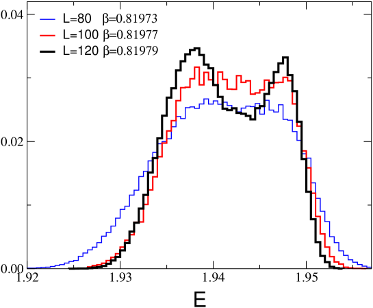
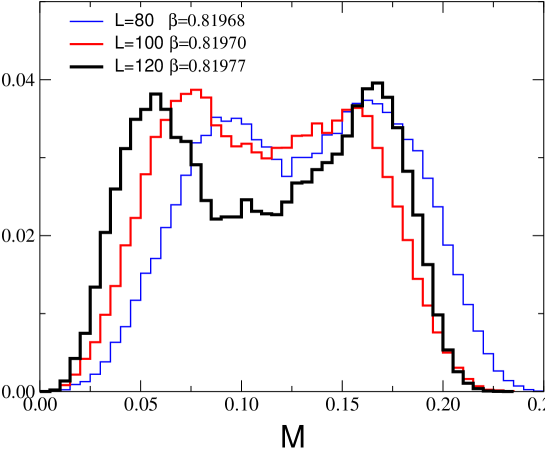
FIG. 8.: Hystograms of the energy density (above) and of the magnetization (below) for $A_{22}=2$ and lattice sizes $L=80$, 100, 120. For each $L$ we report the data for the value of $\beta$ at which the two peaks have approximately the same height. These results have been obtained by reweighting the MC data at $\beta=0.89170$, 0.89175, 0.81980.

E The phase diagram for $A_{22}>A_{4}=1$

In this subsection we investigate the phase diagram of the lattice model (31) for $A_{22}>A_{4}=1$ with the purpose of identifying the regions in which the model shows a first-order or a second-order phase transition.

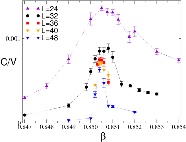
FIG. 9.: Specific heat for $A_{22}=5/2$ and several values of $L$.

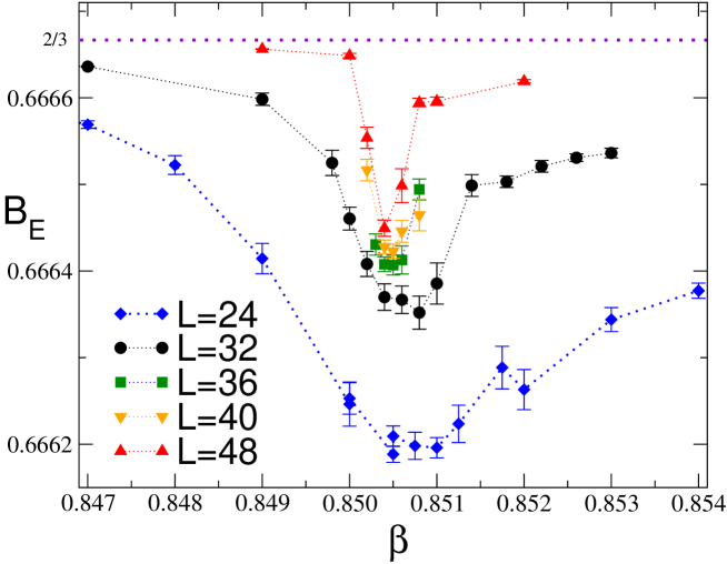
FIG. 10.: Energy cumulant $B_{E}$ for $A_{22}=5/2$ and several values of $L$.

The distributions of $E$ and $M$ show two peaks for $A_{22}\geq 2$ when $L$ is large enough. For $A_{22}=3$ two peaks are already observed for $L=16$, while for $A_{22}=2$ two peaks are observed only for $L\gtrsim 100$, cf. Fig. 8. Thus, the model with $A_{4}=1$ has apparently a relatively strong first-order transition for $A_{22}\gtrsim 3$ that gradually weakens as $A_{22}$ is decreased. In order to check that we are really in the presence of a first-order transition, we check the scaling behavior of the different observables for $L\to\infty$. The predictions for $C$ and $B_{E}$ are well verified. For instance, in Fig. 9 we show $C/V$ for $A_{22}=5/2$ for several values of $L$. In agreement with Eq. (48) $C_{\rm max}/V$ has a finite limit as $L\to\infty$. In Fig. 10 we show the energy cumulant $B_{E}$ for the same value of $A_{22}$; $B_{E,\rm min}$ is different from 2/3, confirming the first-order nature of the transition. From $B_{E,\rm min}$ we can determine the latent heat. For each $L$ we determine $\Delta_{L}$, which is obtained from $B_{E,\rm min}(L)$ by using Eq. (51) and neglecting the $1/V$ corrections. The latent heat is obtained by extrapolating $\Delta_{L}$ assuming $1/V$ corrections.

Estimates of $\Delta_{L}$ for several values of $A_{22}$ and $L$ are reported in Fig. 11. They show the expected $1/V$ behavior and allow a precise determination of the latent heat in the infinite-volume limit. The results of the extrapolations are reported in Table II. They are in perfect agreement with those obtained from the maximum of the specific heat, using Eq. (48), and from the position of the peaks in the energy distributions.

We have also performed MC simulations for $A_{22}=5/3$ and 7/5 on lattices of size $L\leq 120$, without observing evidences for first-order transitions. The hystograms of $E$ and $M$ do not show any evidence of two peaks and are not significantly broad, as for instance the distribution of $E$ for $L=80$ and $A_{22}=2$, cf. Fig. 8, which would indicate the onset of two peaks. In the cases $A_{22}=5/3,7/5$, $C$ and $B_{E}$ on lattices of size $L\leq 120$ do not show the behavior predicted by the phenomenological theory of first-order transitions [66]. In particular, $B_{E,\rm min}$ continuously increases towards 2/3 and we can only put upper bounds on $\Delta_{h}$. For $A_{22}=5/3$ we obtain for instance $\Delta_{h}<0.005$. A more stringent bound is suggested by the width of the energy distribution at $\beta_{c}$, i.e. $\Delta_{h}<0.003$.

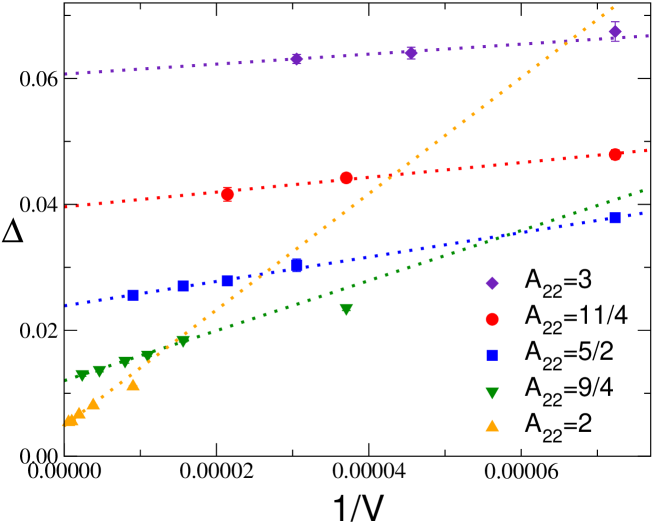
FIG. 11.: Values of $\Delta_{L}$ for $A_{22}=2$, 9/4, 5/2, 11/4, 3, as obtained from $B_{E,{\rm min}}$ by using Eq. (51). The lines represent the infinite-volume extrapolations assuming a $1/V$ asymptotic correction.

TABLE II.: For the model with $A_{4}=1$ and several values of $A_{22}$ we report $s_{L}$, $\beta_{c}$, the average energy density $E_{c}\equiv(E_{+}+E_{-})/2$, $\Delta$, cf. Eq. (52), and the latent heat $\Delta_{h}$. For $\beta_{c}$ and $E_{c}$ all reported digits are exact.

$A_{22}$	$s_{L}$	$\beta_{c}$	$E_{c}$	$\Delta$	$\Delta_{h}$
3	1	0.8733	1.98	0.0607(6)	0.1198(12)
11/4	14/15	0.8627	1.98	0.0396(12)	0.0783(24)
5/2	6/7	0.8504	1.97	0.0239(4)	0.0471(8)
9/4	10/13	0.8364	1.96	0.0120(4)	0.0235(8)
2	2/3	0.8198	1.94	0.0048(2)	0.0093(4)
5/3	1/2	0.7927	1.92	$<$ 0.0015	$<$ 0.003

Let us now discuss the behavior of the variables related to the magnetization. In particular, we focus on the derivatives with respect to $\beta$ of $B_{1}$ and $B_{2}$. Predictions (55) and (56) are well verified by our data with $A_{22}\geq 2$. We observe the presence of a peak in $B_{1}$ at fixed $L$ that becomes sharper as $L$ increases and we also verify that far from this peak Eq. (56) holds. Of course, corrections increase as $A_{22}$ decreases, as expected. On the other hand, $B_{1}$ is monotonically decreasing with $\beta$ at fixed $L$ for $A_{22}=7/5$ and $A_{22}=5/3$, providing no evidence that the transition is of first order for these two values of $A_{22}$.

We have repeated the same analysis for $B_{2}$. Its behavior looks quite different with respect to $B_{1}$. First of all, we observe a monotonic behavior without peaks for all the considered values of $A_{22}$, including the largest ones for which the peak in $B_{1}$ is rather sharp. Moreover, the data are reasonably well described by assuming

$${dB_{2}\over d\beta}=\hat{f}(B_{1}),$$ (57)

suggesting that $B_{2}$ does not have a jump at the transition, as expected on the basis of the argument presented at the end of Sec. IV D. A similar analysis can also be performed for $l_{\xi}$ for which we have no prediction. Our data are roughly consistent with a behavior of the form

$${dl_{\xi}\over d\beta}=L^{\theta}\hat{f}(B_{1})$$ (58)

with $3.2\lesssim\theta\lesssim 3.7$. It is quite difficult to intepret such a value of $\theta$ that could well be $d$ or $d+1$ depending on the size of the corrections.

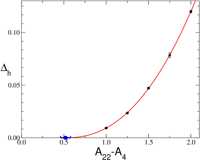
FIG. 12.: Latent heat $\Delta_{h}$ versus $A_{22}$. The line corresponds to the best fit, $\Delta_{h}=0.049(A_{22}-1.52)^{2.29}$. We also report the estimate of $A_{22}^{*}$ with the corresponding error: $A_{22}^{*}=1.52(6)$.

The results for $\Delta_{h}$ reported in Fig. 12 suggest therefore a phase diagram characterized by a line of first-order transitions extending from large values of $A_{22}$ down to $A_{22}^{*}$ where $\Delta_{h}$ vanishes. In order to compute $A_{22}^{*}$, we should first discuss the expected behavior of $\Delta_{h}$ close to the tricritical point $A_{22}^{*}$ (see, e.g., Ref. [76]). We consider a generic model depending on two parameters $\beta$ and $g$ with a tricritical point at $g^{*}$, $\beta^{*}_{c}\equiv\beta_{c}(g^{*})$. The critical behavior can be parametrized in terms of two linear scaling fields $u_{1}$ and $u_{2}$ with RG dimensions $y_{1}$ and $y_{2}$, satisfying $y_{1}>y_{2}$. In the absence of any symmetry, the linear scaling fields are combinations of $(g-g^{*})$ and of $(\beta-\beta_{c}^{*})$. The scaling field $u_{1}$ is completely defined, while $u_{2}$ can be arbitrarily chosen as long as it is independent of $u_{1}$. Therefore, we write

$$u_{1} = a_{1}(\beta-\beta_{c}^{*})+a_{2}(g-g^{*}),$$ (59)

$$u_{2} = g-g^{*}.$$ (60)

The first-order transition line is characterized by the equation $u_{2}=c_{1}u^{y_{2}/y_{1}}_{1}$ with, by a proper choice of the scaling field, $u_{1}>0$. Analogously, the second-order transition line is given by $u_{2}=c_{2}(su_{1})^{y_{2}/y_{1}}$ where $s$ may be either 1 or $-1$ and $|c_{1}|\not=|c_{2}|$. Note that both lines are tangent to $u_{1}=0$, but that the nonanalytic deviations are parametrized differently.

The free energy can be written as

$$F\approx F_{\rm reg}(\beta,g)+|u_{2}|^{d/y_{2}}F_{\rm sing,\pm}(u_{1}|u_{2}|^{-y_{1}/y_{2}}),$$ (61)

where $F_{\rm sing,+}$ (resp. $F_{\rm sing,-}$) applies to the case $u_{2}>0$ (resp. $u_{2}<0$), and $F_{\rm reg}(\beta,g)$ is a regular function. By hypothesis, assuming $c_{1}>0$ without loss of generality, $F_{\rm sing,+}(x)$ is continuous but has a discontinuous derivative at the first-order transition line, i.e. for $x=c_{1}^{-y_{1}/y_{2}}$. It follows

$$E_{+}-E_{-}\approx a_{2}|u_{2}|^{(d-y_{1})/y_{2}}\Delta F_{\rm sing,+}^{\prime}\sim|g-g^{*}|^{(d-y_{1})/y_{2}}.$$ (62)

In the model we consider $g=A_{22}$, so that we predict that sufficiently close to the tricritical point $A_{22}^{*}$

$$\Delta_{h}=\Delta_{0}(A_{22}-A_{22}^{*})^{\theta},$$ (63)

where $\theta$ is an exponent defined by the tricritical theory. If we fit our data for the latent heat with this expression we obtain

$$A_{22}^{*}=1.52(6),\qquad\qquad\Delta_{0}=0.049(7),\qquad\qquad\theta=2.29(15),$$ (64)

with a $\chi^{2}$ per degree of freedom (DOF) of 0.24. The fit is stable with respect to the number of points that are included: If the point with $A_{22}=3$ is not included we obtain $A_{22}^{*}=1.50(12)$ and $\theta=2.35(36)$, in full agreement with the result reported above. We have also investigated the possibility that $A_{22}^{*}=A_{4}=1$, which would imply the absence of critical transitions in the O(2)$\otimes$O(2) universality class. A fit of the data for the latent heat of the form $\Delta_{h}=\Delta_{0}(A_{22}-1)^{\theta}$ gives $\theta=3.49(4)$ with $\chi^{2}/$DOF $\approx 9$. If the point with $A_{22}=3$ is not included we obtain $\theta=3.87(4)$ ($\chi^{2}/$DOF $\approx 11$), while if the two points with largest $A_{22}$ are discarded we obtain $\theta=4.00(3)$ ($\chi^{2}/$DOF $\approx 9$). These fits are significantly worse than that presented above. Moreover, the estimate of $\theta$ does not agree with the theoretical prediction that can be obtained assuming the tricritical point to be at $A_{22}=1$. Indeed, if $A_{22}^{*}=1$ the tricritical theory coincides with the O(4) theory. There are two relevant perturbations, the thermal perturbation with RG dimension $1/\nu$ and the perturbation that breaks the O(4) symmetry down to O(2)$\otimes$O(2), which is associated in field theory with the spin-4 quartic operator, with RG dimension $\phi/\nu$. For the O(4) universality class, $\alpha=-0.247(6)$ (Ref. [61]) and $\phi=0.08(1)$ (Ref. [48]). Since $\phi<1$ in this case, we have $y_{1}=1/\nu$ and $y_{2}=\phi/\nu$, so that we should have [77]

$$\Delta_{h}\sim(A_{22}-1)^{(1-\alpha)/\phi}\sim(A_{22}-1)^{16\pm 2},$$ (65)

which is not compatible with the MC results. Thus, our results are incompatible with $A_{22}^{*}=1$, unless the limiting behavior sets in for even smaller values of $\Delta_{h}$. This seems unlikely, since for $A_{22}\lesssim 3$ we are already in a region in which $\Delta_{h}\ll 1$. Thus, our simulations provide a nice evidence in favor of the existence of a tricritical point at $A_{22}^{*}>1$ separating the first-order transition line from a continuous transition line for $1<A_{22}<A_{22}^{*}$. Notice that a phase transition is always expected due to the qualitative difference of the minimum of the free energy in the high- and low-temperature regions.

The estimate (64) implies that for $A_{22}=5/3$ one should observe a first-order transition. As we have already discussed, our data do not show any evidence for that. This is hardly surprising, since the fit of the estimates of $\Delta_{h}$ predicts $\Delta_{h}=0.8(6)\cdot 10^{-3}$ for $A_{22}=5/3$, which is smaller than the bound $\Delta_{h}<3\cdot 10^{-3}$ obtained on lattices $L\leq 100$. A posteriori, however, one can convince oneself of the first-order nature of the transition by considering the estimated values of $\nu$. For instance, the derivative of the Binder parameter $B_{1}$ with respect to $\beta$ is expected to scale at the critical point as $B_{1}^{\prime}\sim L^{d}$ for a first-order transition. In our analyses of the data with $A_{22}\geq 2$, we find that, if one estimates $B_{1}^{\prime}$ with $B_{1}^{\prime}\sim L^{\theta}$, the effective $\theta$ rapidly increases towards $d$ as the considered set of sizes increases, even when a double peak in the distributions is not yet evident. For $A_{22}=5/3$ if we use the data with $L\geq 60$ we obtain $1/\theta=0.47(2)$, while including only the data with $L\geq 80$ gives $1/\theta=0.42(4)$: the exponent $\theta$ is increasing towards the expected value $\theta=d=3$. At a second-order transition one expects $B_{1}^{\prime}\sim L^{1/\nu}$, and thus the previous results would give a quite small value for $\nu$, definitely incompatible with the FT predictions. Therefore, even if we do not have a direct evidence, the data for $A_{22}=5/3$ are better explained by a very weak first-order transition than by a second-order one.

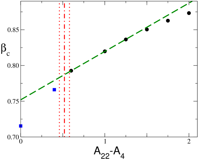
FIG. 13.: The inverse critical temperature $\beta_{c}$ versus $A_{22}$. The vertical lines indicate the estimate of $A_{22}^{*}$ with its error. The data for $A_{22}>A_{22}^{*}=1.52(6)$ are indicated by circles, while the ones for $A_{22}<A_{22}^{*}$ are indicated by a square. Errors are much smaller than the size of the symbols. The dashed line shows the linear fit of the three data for $A_{22}>A_{22}^{*}$ that are closest to $A_{22}^{*}$.

The presence of a tricritical point at $A_{22}^{*}=1.52(6)$ is further supported by the results for $\beta_{c}$ reported in Table II and plotted in Fig. 13 versus $A_{22}-A_{4}$. Equation (60) implies that, sufficiently close to the tricritical point $A_{22}^{*}$, the values of $\beta_{c}$ along the first-order transition line behave as

$$\beta_{c}-\beta_{c}^{*}\approx-{a_{2}\over a_{1}}(A_{22}-A_{22}^{*})+{1\over a_{1}}\left[{1\over c_{1}}(A_{22}-A_{22}^{*})\right]^{y_{1}/y_{2}},$$ (66)

while, along the second-order transition line, we have similarly

$$\beta_{c}-\beta_{c}^{*}\approx-{a_{2}\over a_{1}}(A_{22}-A_{22}^{*})+{1\over sa_{1}}\left[{1\over c_{2}}(A_{22}-A_{22}^{*})\right]^{y_{1}/y_{2}},$$ (67)

Equations (66) and (67) strictly hold only if $y_{1}/y_{2}<2$, otherwise one should also include additional integer powers $(A_{22}-A_{22}^{*})^{n}$, $n<y_{1}/y_{2}$, with coefficients that are identical for the first-order and second-order transition line.

The linear dependence of $\beta_{c}$ on $A_{22}$ for $A_{22}\gtrsim A_{22}^{*}$ is clearly observed in Fig. 13. A linear fit of the three points that are closest to $A_{22}^{*}$ and satisfy $A_{22}>A_{22}^{*}$ gives $a_{2}/a_{1}\approx-0.068$ with a reasonable $\chi^{2}$. Note that the deviations from a straight line are very small, indicating that the corrections, and in particular, the nonanalytic ones, are tiny. Fig. 13 also shows the value of $\beta_{c}$ for $A_{22}=7/5<A_{22}^{*}$, i.e. $\beta_{c}=0.76615(15)$ which will be determined in the next subsection, and for the O(4) $\phi^{4}$ model obtained by setting $A_{22}=A_{4}=1$, which is given by $\beta_{c}=0.7154(1)$ [78]. Both values, and in particular the one for $A_{22}=7/5$, differ significantly from the linear extrapolation of the data for $A_{22}>A_{22}^{*}$. This behavior of $\beta_{c}$ as a function of $A_{22}$ is naturally explained by the presence of a tricritical point at $A_{22}^{*}=1.52(6)$, and it is another evidence of the fact that the point $A_{22}=7/5$ belongs to the second-order transition region. Indeed, in this scenario the nonanalytic corrections are different ($|c_{2}|\not=|c_{1}|$) from those observed in the first-order transition region. Thus, the observed value for $A_{22}=7/5$ can be explained by the presence of nonanalytic corrections to the linear behavior that are substantially larger ($|c_{2}|\ll|c_{1}|$) than those observed on the side of the first-order transition line. The data shown in Fig. 13 can hardly be explained by assuming $A_{22}^{*}=1$, i.e. a first-order transition line extending down to the O(4) point $A_{22}=A_{4}=1$. Indeed, in this case the linear behavior should extend down to the O(4) point, but this is clearly contradicted by the values of $\beta_{c}$ obtained for $A_{22}=7/5$ and $A_{22}=1$. Note also that the same RG arguments leading to Eqs. (60), (61) and (66) tell us that the values of $\beta_{c}$ along the continuous transition line must approach linearly the O(4) point $A_{22}=A_{4}$, but with a slope different from the one observed at the tricritical point $A_{22}^{*}=1.56(2)$.

In conclusion we have shown that, in the quartic parameter space with $A_{22}>A_{4}$, there is a region in which the transition is continuous and therefore belongs to the O(2)$\otimes$O(2) universality class controlled by the O(2)$\otimes$O(2) FP found in the FT approach of Sec. II.

Finally, we should note that in the FT studies the basin of attraction of the O(2)$\otimes$O(2) FP includes all theories with $s<s^{*}$ and $s^{*}\gtrsim 1$, while here $s^{*}_{L}=0.41(4)$. As we have already discussed before, in spite of the similar definition, $s_{L}$ should not be identified with $s$ and we have $s_{L}\to s$ only for a weakly coupled theory, i.e. for $A_{4}\to 0$ and $A_{22}\to 0$. Here, $A_{4}=1$, so that we are far from this limiting case. In any case, the FT results imply that $s^{*}_{L}$ increases if $A_{4}$ decreases. The critical value $s^{*}_{L}$ is also expected to increase if longer-range interactions are added. Indeed, as shown in App. B, we expect $0.71\lesssim s^{*}_{L}<1.23$ for medium-range models with $A_{4}=1$.

F Determination of the critical quantities for $A_{22}=7/5$

In this Section we analyze the results for $A_{22}=7/5$. On the basis of the analysis presented in the previous Section, in this case the transition should be of second order. In the FSS limit we expect the following behavior

$$R\approx f_{R}[(\beta-\beta_{c})L^{1/\nu}],$$ (68)

$$\chi\approx L^{2-\eta}f_{\chi}[(\beta-\beta_{c})L^{1/\nu}],$$ (69)

$$M\approx L^{-\beta/\nu}f_{M}[(\beta-\beta_{c})L^{1/\nu}],$$ (70)

where $R$ is any RG invariant quantity (we will take $R$ to be $B_{1}$, $B_{2}$, or $l_{\xi}$). These scaling forms are valid for $\beta\to\beta_{c}$, $L\to\infty$ at fixed argument $(\beta-\beta_{c})L^{1/\nu}$. From Eq. (68) we obtain moreover

$${dR\over d\beta}\approx L^{1/\nu}f_{R}^{\prime}[(\beta-\beta_{c})L^{1/\nu}].$$ (71)

Eqs. (69), (70), and (71) can be used to determine $\eta$, $\beta/\nu$, and $\nu$. It is also possible to avoid the use of the two unknown quantities, $\beta_{c}$ and $\nu$. We use Eq. (68) to express $(\beta-\beta_{c})L^{1/\nu}$ in terms of $R$, and rewrite all equations as

$$\chi\approx L^{2-\eta}g_{\chi,R}(R),$$ (72)

$$M\approx L^{-\beta/\nu}g_{M,R}(R),$$ (73)

$${dR_{1}\over d\beta}\approx L^{1/\nu}g_{R_{1},R_{2}}(R_{2}),$$ (74)

where $R$ is a RG-invariant quantity.

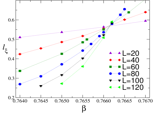
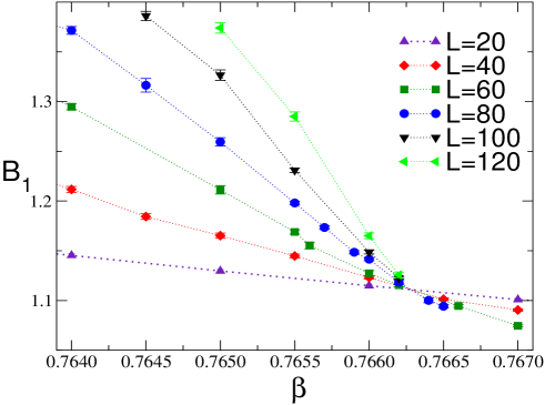
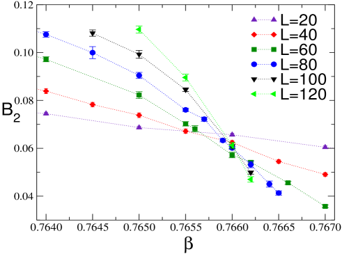
FIG. 14.: Plots of $l_{\xi}$, $B_{1}$, and $B_{2}$ for $A_{22}=7/5$. The lines are drawn to guide the eye.

Let us begin by performing a direct analysis of $B_{1}$, $B_{2}$, and $l_{\xi}$. We fit our results corresponding to $20\leq L\leq 120$ and $0.755\leq\beta\leq 0.767$ (see Fig. 14) by using Eq. (68). For this purpose we must somehow parametrize the scaling function $f_{R}(x)$. We use a simple polynomial expression, writing

$$f_{R}(x)=\sum_{n=0}^{p}a_{n}x^{n}.$$ (75)

The order $p$ is chosen in the following way. For a given set of data we perform a nonlinear fit, increasing each time $p$ until the $\chi^{2}$ changes by approximately 1 by going from $p$ to $p+1$. Of course, one should also worry about scaling corrections and crossover effects. In order to detect them we perform the fit several times, each time including only the data corresponding to lattice sizes $L$ larger than some value $L_{\rm min}$. The corresponding results are reported in Table III.

TABLE III.: Analysis of the RG-invariant quantities $R$, $R=B_{1}$, $B_{2}$, and $l_{\xi}$, by using Eq. (68). We report $\nu$, $\beta_{c}$, and $R^{*}=R(\beta_{c})$.

$R$	$L_{\rm min}$	$\chi^{2}$/DOF	$\nu$	$\beta_{c}$	$R^{*}$
$B_{1}$	20	78/70	0.728(4)	0.766284(8)	1.1111(6)
	40	63/54	0.716(7)	0.766278(11)	1.1121(9)
	60	40/38	0.711(14)	0.766281(17)	1.1121(16)
	80	24/20	0.665(27)	0.766260(25)	1.1148(30)
$B_{2}$	20	305/69	0.662(5)	0.765890(7)	0.0643(2)
	40	92/54	0.639(9)	0.765992(10)	0.0604(4)
	60	51/38	0.650(17)	0.766044(15)	0.0580(7)
	80	25/21	0.587(33)	0.766038(19)	0.0585(9)
$l_{\xi}$	20	117/71	0.687(2)	0.766153(3)	0.5692(6)
	40	61/55	0.692(2)	0.766168(5)	0.5726(10)
	60	29/37	0.694(5)	0.766181(8)	0.5770(19)
	80	9/18	0.673(13)	0.766168(12)	0.5741(39)

The quality of the fits of $B_{1}$ and $l_{\xi}$ is reasonably good ($\chi^{2}$/DOF $\approx 1$), while for $B_{2}$ one should certainly discard the results with $L_{\rm min}=20$ and 40. As far as the estimates of $\nu$ are concerned, we observe in all cases a systematic drift. The analyses of $B_{1}$ and $l_{\xi}$ give first $\nu\approx$ 0.69 - 0.71 and then, by using only the data with $L_{\rm min}=80$, one obtains $\nu\approx 0.66$-0.67. On the other hand, fits of $B_{2}$ give first $\nu\approx 0.66$ and then, for $L_{\rm min}=80$, $\nu\approx 0.59$, although with a large error of $\pm 0.03$. Clearly the data are affected by large scaling corrections and, apparently, even on these relatively large lattices one is not able to obtain a precise estimate of $\nu$, but only an upper bound $\nu\lesssim 0.67$. In any case, if we assume that the observed discrepancies give a reasonable estimate of the systematic error, the results with $L_{\rm min}=80$ give

$$\nu=0.63(7),$$ (76)

which includes the estimates from $B_{1}$, $B_{2}$, and $l_{\xi}$ with their errors. This is fully compatible with the FT estimates.

The results obtained from the analysis can be interpreted in terms of a crossover due to the presence of a nearby O(4) FP. Indeed, the observed behavior rensembles quite closely what is observed in field theory for, say, $s=1/4$. The effective exponent $\nu$ is first close to the O(4) value and then decreases towards its asymptotic value. This interpretation is somehow supported by the observed values of $B_{1}^{*}$ and $l_{\xi}^{*}$, where $R^{*}=R(\beta_{c})$. They are close to the corresponding O(4) ones [61]: $l^{*}_{\xi}\approx 0.547$, $B_{1}^{*}=1.0945(2)$. Only for $B_{2}$ do we observe a relatively large difference since in the O(4) case $B_{2}^{*}={1\over 12}B_{1}^{*}=0.09121(2)$. This may explain why the estimates of $\nu$ from $B_{2}$ are those that most differ from the O(4) ones. Of course, one may not exclude that the asymptotic values $B_{1}^{*}$ and $l_{\xi}^{*}$ are close to the O(4) estimates.

As a check we have also considered the derivatives of $B_{1}$, $B_{2}$, and $l_{\xi}$ and we have used Eq. (74). We find that in all cases the best fit (smallest $\chi^{2}$/DOF) is obtained by taking $R_{1}=R_{2}$ with results that are (not surprisingly) fully compatible with those obtained in the previous analysis. Fits with $R_{1}\not=R_{2}$ are somewhat worse but always show the same pattern. While for small values of $L_{\rm min}$, $\nu$ varies between 0.64 and 0.70, depending on the choice of $R_{1}$ and $R_{2}$, for $L_{\rm min}=80$ the analyses indicate a smaller value, fully compatible with the result reported above.

The analyses of $B_{1}$, $B_{2}$, and $l_{\xi}$ also provide estimates of $\beta_{c}$. There is a clear upward trend in the estimates obtained from $B_{2}$, as it can be also understood from Fig. 14: the value at which the lines $B_{2}(\beta,L)$ at fixed $L$ cross moves significantly towards higher values of $\beta$ as $L$ increases. The estimates obtained from $B_{1}$ and $l_{\xi}$ are apparently stable, but not compatible within the tiny statistical errors indicating that there are strong (compared to the statistical errors) crossover effects, as observed for $\nu$. If we assume that the discrepancies among the estimates obtained from the analyses of the three RG-invariant quantities give a reasonable estimate of the systematic error, an estimate of $\beta_{c}$ that includes all results is

$$\beta_{c}=0.76615(15).$$ (77)

We finally compute $\eta$ and $\beta/\nu$ from the analysis of $\chi$ and $M$. We have performed the analyses by using Eqs. (72) and (73). The analyses using $R=l_{\xi}$ are well behaved and show little dependence on $L_{\rm min}$, leading to the estimates

$$\eta=0.045(10),\qquad\qquad{\beta\over\nu}=0.0525(10).$$ (78)

The corresponding scaling plots are reported in Fig. 15. On the other hand we observe systematic deviations if we use $R=B_{1}$ or $B_{2}$. The goodness of the fit, $\chi^{2}$/DOF, is a factor of ten larger than for the analysis with $R=l_{\xi}$, and the estimates vary significantly, between $-0.1$ and 0.2 ($\eta$) and 0.45 and 0.6 ($\beta/\nu$).

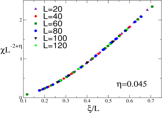
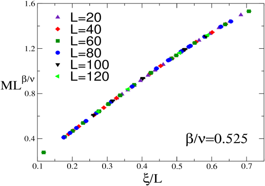
FIG. 15.: Plots of $\chi/L^{2-\eta}$ (above) and of $ML^{\beta/\nu}$ (below) vs $\xi/L$. Here $\eta=0.045$ and $\beta/\nu=0.525$.

The results (78) satisfy the scaling relation $2\beta/\nu=1+\eta$ quite precisely. They can be compared with the FT results: $\eta=0.09(1)$ (MZM scheme, Ref. [19]) and $\eta=0.09(4)$ ($\overline{\rm MS}$ scheme). Although larger, the $\overline{\rm MS}$ estimate is compatible within error bars. A discrepancy is observed for the MZM result, whose error might have been underestimated (after all, the MZM series are not Borel summable). Of course, it is also possible that scaling corrections play an important role, as it is the case in the analyses of $B_{1}$, $B_{2}$, and $l_{\xi}$. In this case, we expect the MC result to be influenced by the presence of the nearby O(4) FP. Such an interpretation is supported by the fact that the estimated $\eta$ is close to the O(4) result $\eta=0.0365(10)$ (Ref. [61]).

Finally, we analyzed the specific heat by using

$$C=L^{\alpha/\nu}f(R),$$ (79)

which is valid as long as $\alpha>0$. We do not expect this fit to be very precise since we are neglecting the analytic contribution that gives rise to corrections of order $L^{-\alpha/\nu}$, which are expected to be sizeable since $\alpha$ is small. All fits have a poor $\chi^{2}$. Only the fit with $R=l_{\xi}$ and $L_{\rm min}=80$ has $\chi^{2}$/DOF of order one. Fits using $l_{\xi}$ give estimates of $\alpha/\nu$ that decrease as $L_{\rm min}$ increases, varying between 0.20 and 0.16. Fits using $B_{1}$ show the same decreasing trend with $0.19\lesssim\alpha/\nu\lesssim 0.20$. Fits using $B_{2}$—they have a very large $\chi^{2}$, $\chi^{2}$/DOF = 14 for $L_{\rm min}=80$—show a more erratic behavior with $L_{\rm min}$ and give $0.14\lesssim\alpha/\nu\lesssim 0.18$. We quote as final result that obtained by using $l_{\xi}$ and $L_{\rm min}=80$:

$${\alpha\over\nu}=0.16(3).$$ (80)

The error has been chosen such that it includes all estimates with $L_{\rm min}=80$. Using hyperscaling Eq. (80) gives $\nu=0.63(1)$, in good agreement with the result reported above, and $\alpha=0.10(2)$. A scaling plot is reported in Fig. 16.

The very large $\chi^{2}$/DOF of the above-reported analysis is probably due the fact that the analytic contribution to the specific heat is neglected. We have thus performed a second set of analyses using

$$C=L^{\alpha/\nu}f_{1}(R)+f_{2}(\beta)$$ (81)

and $R=\xi/L$. As before, we have used polynomials for $f_{1}(x)$ and $f_{2}(x)$. Fifth-order polynomials allow us to obtain $\chi^{2}$/DOF $\approx 1$ even for $L_{\rm min}=20$. We obtain $\alpha/\nu=-0.10(6)$, $0.01(9)$, and $0.16(25)$ for $L_{\rm min}=20$, 40, 60 respectively. The results for the largest $L_{\rm min}$ are compatible with the estimates reported above. However, the very large errors indicate that our data are not precise enough and that our set of values of $L$ is too small to disentangle the analytic background from the singular behavior. This probably means that the error reported in Eq. (80) should not be taken too seriously and is most likely underestimated.

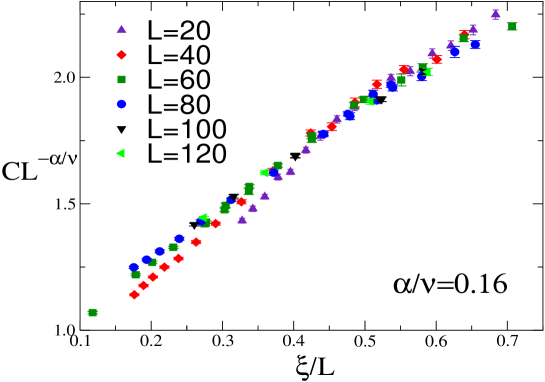
FIG. 16.: Plot of $C/L^{\alpha/\nu}$ vs $\xi/L$. Here $\alpha/\nu=0.16$.

V Conclusions

In this paper we investigated the critical behavior of three-dimensional models with symmetry O(2)$\otimes$O($N$) described by the FT Hamiltonian (1) in the case $v_{0}>0$, which corresponds to the symmetry-breaking pattern O(2)$\otimes$O($N$)$\to$O(2)$\otimes$O($N-2$) (the case $v_{0}<0$ has been discussed in detail in Ref. [11]).

First, we considered the FT perturbative approach. The analysis of the five-loop series in the $\overline{\rm MS}$ scheme without $\epsilon$ expansion provides strong evidence for the presence of a stable FP with $v>0$ for $N=2$ and $N=3$, and therefore for the existence of the corresponding three-dimensional O(2)$\otimes$O($N$) universality classes. This result confirms the conclusions of Ref. [19], in which a stable FP with $v>0$ was found in the three-dimensional MZM scheme. Note that these FT perturbative analyses disagree with the conclusions of Refs. [30, 31, 5], in which no FP was found by using a nonperturbative RG approach. Moreover, the $\overline{\rm MS}$ scheme without $\epsilon$ expansion allowed us to obtain fixed-dimension results at any $d$. We recovered the $\epsilon$-expansion results sufficiently close to four dimensions and obtained a full picture of the fate of the different FPs as $d$ varies from four to three dimensions.

In order to confirm the existence of a new universality class we have performed a MC study of a lattice discretization of Hamiltonian (1) for $N=2$. The purpose is to identify a parameter region in which the transition is of second order with the expect symmetry-breaking pattern, O(2)$\otimes$O(2)$\to$O(2). A detailed analysis of the critical behavior of the model (3) for $A_{4}=1$ and $A_{22}>A_{4}$ shows the following phase diagram. For $A_{22}>A_{22}^{*}=1.52(6)$ the model has a first-order transition. Such a transition is easily identified for $A_{22}\gtrsim 3$—the energy and the magnetization show two peaks already for $L\approx 10$ with reduced latent heat $\Delta E/T_{c}$ larger than 0.1. The first-order transition becomes weaker as $A_{22}$ decreases, the latent heat vanishing at the tricritical point $A_{22}=A_{22}^{*}$. For $1=A_{4}<A_{22}<A_{22}^{*}$ the transition is continuous. Its critical behavior is expected to belong to the three-dimensional O(2)$\otimes$O(2) universality class and therefore to be controlled by the stable FP of the O(2)$\otimes$O(2) theory found within the FT methods. We have also performed simulations of the lattice model for $A_{22}=7/5$ in order to identify the critical behavior. All results are definitely compatible with the expected behavior at a second-order transition. We are however unable to provide precise estimates of the critical exponents since we observe strong crossover effects, probably due to the presence of the nearby O(4) FP. The effective exponents computed in the MC simulation rensemble those observed in the FT model for small $s\equiv v_{0}/u_{0}$, see Fig. 7, indicating that crossover effects play an important role in these systems and make difficult, both numerically and experimentally, a precise determination of the asymptotic critical behavior.

The FT Hamiltonian (1) is supposed to describe the critical behavior of STA’s and of helimagnets [3]. Inelastic neutron-scattering experiments show that STA’s can be modeled by three-component spin variables $\vec{s}$ associated with each site of a stacked triangular lattice and by the Hamiltonian

$${\cal H}_{\rm STA}=J_{\|}\sum_{\langle vw\rangle_{xy}}\vec{s}(v)\cdot\vec{s}(w)+J_{\bot}\,\sum_{\langle vw\rangle_{z}}\vec{s}(v)\cdot\vec{s}(w)+D\sum_{v}s_{3}(v)^{2}.$$ (82)

The first sum is over nearest-neighbor pairs within the triangular layers ($xy$ planes) with an antiferromagnetic coupling $J_{\|}<0$, the second one is over orthogonal interlayer nearest neighbors. If the uniaxial term is positive, one has an effective two-component theory. Numerically, Hamiltonian (82) has been much studied in the limiting cases $D=+\infty$ and $D=0$. In the first case the spins are confined to a plane, i.e., one is effectively considering XY spins. There is now evidence that XY STA’s undergo first-order transitions, at least for $|J_{\bot}/J_{\|}|$ not too small. Indeed, first-order behavior has been observed for $J_{\bot}/J_{\|}=-3/4$ (Ref. [33]), $J_{\bot}/J_{\|}=-1$ (Ref. [34]), and $J_{\bot}/J_{\|}=-10$ (Ref. [32]). The numerical results indicate that the first-order transition becomes stronger as $|J_{\bot}/J_{\|}|$ increases, and thus we can conclude that all these models have first-order transitions, at least for $|J_{\bot}/J_{\|}|\gtrsim 3/4$. It should however be noted that the latent heat is very small. For $J_{\bot}/J_{\|}=-3/4$ and $J_{\bot}/J_{\|}=-1$, $\Delta E/T_{c}\approx 7\cdot 10^{-3}$ [33, 34]. This means that small modifications of the lattice model may turn the first-order transition into a second-order one. In particular, it is not clear whether, on the basis of these numerical simulations of the XY STA’s, we should expect first-order transitions also for experimental easy-plane systems, which do not satisfy the condition $D\gg J_{\|},|J_{\bot}|$. For instance, in the case of CsMnBr₃ we have [1] $J_{\|}\approx 0.0018$ meV, $J_{\bot}=0.88$ meV, and $D=0.013$ meV, while in other compounds like CsVX₃ (X = Cl, Br, I) one observes [1] $D\approx J_{\|}\ll J_{\bot}$. O(2)$\otimes$O(2) critical behavior is also expected in easy-axis materials ($D<0$) in the presence of a (large) magnetic field along the easy direction.

Experiments on STA’s favor a second-order transition, although the estimates of $\beta$ do not satisfy the inequality $\beta\geq\nu/2$ that is expected on the basis of unitarity [31, 5]. Of course, this could be explained by the presence of a weak first-order transition. A second possibility is that the experimental systems are in the basin of attraction of the stable FP, but close to the boundary of the stability region. If this is the case, on the basis of the FT crossover analysis, one expects strong crossover effects; see, for example, the results presented in Fig. 7 for $s\approx 1$. Thus, the exponents $\beta$ and $\nu$ that are measured experimentally may well differ from their asymptotic value. For what concerns helimagnets, their critical behavior is somewhat different from that observed in STA’s. The exponent $\beta$ is always very close to the O(4) value, while $\alpha$ varies between 0.1 and 0.3. These results strongly remind our MC ones with $A_{22}=7/5$. In that case, $\beta/\nu$ was close to the O(4) value and $\alpha\approx 0.10$. Thus, the helimagnetic results can be explained by the presence of the nearby O(4) FP that controls the critical behavior for $|t|\gtrsim 10^{-3}$.

Finally, we would like to conclude with some remarks on the experimental relevance of the O(2)$\otimes$O(3) universality class. Such a critical behavior is expected in some easy-axis materials that have a small uniaxial anisotropy [1], for instance in RbNiCl₃, VCl₂, and VBr₂. However, the reduced-temperature region in which O(2)$\otimes$O(3) behavior might be observed is usually very small, i.e. for $t\gtrsim 10^{-2}$, because these systems are expected to crossover to an XY critical behavior for $t\lesssim 10^{-2}$ [1, 3]. Therefore, the asymptotic O(2)$\otimes$O(3) critical behavior can be hardly observed in these materials and significant differences between theoretical predictions and experimental results should not be unexpected. As argued in Ref. [79], and usually assumed in the literature, the O(2)$\otimes$O(3) critical behavior should also be experimentally realized in easy-axis STA’s, such as CsNiCl₃ and CsNiBr₃, at the multicritical point observed in the presence of an external magnetic field along the easy axis, or at the critical concentration of mixtures of easy-axis and easy-plane materials, for instance in CsMn(Br_xI${}_{1-x})_{3}$ [80]. We note that the identification of the multicritical point with the O(2)$\otimes$O(3) universality class is not obvious and should be theoretically analyzed. The critical behavior at the multicritical point in a magnetic field should be described by the stable FP of the most general LGW theory with symmetry O(2)$\otimes$[${\mathbb{Z}}_{2}\oplus$O(2)] [81]. In Ref. [79] only the quadratic terms have been considered and discussed, but the relevant LGW Hamiltonian has also additional quartic terms beside those appearing in the O(2)$\otimes$O(3) Hamiltonian. As a consequence, the O(2)$\otimes$O(3) FP, describing a critical behavior with an enlarged O(2)$\otimes$O(3) symmetry, determines the asymptotic behavior at the multicritical point only if it remains stable with respect to the additional quartic terms breaking O(2)$\otimes$O(3) to O(2)$\otimes$[${\mathbb{Z}}_{2}\oplus$O(2)]. The critical behavior at the multicritical point is determined by the stable FP of the RG flow of the complete LGW theory with symmetry O(2)$\otimes$[${\mathbb{Z}}_{2}\oplus$O(2)]. This issue was recently investigated in Ref. [81] by a FT analysis based on five-loop calculations within the $\overline{\rm MS}$ and MZM schemes. Unfortunately, this study was unable to establish the stability properties of the O(2)$\otimes$O(3) FP. In any case, it did not provide evidence for any other stable FP. Thus, on the basis of these FT results, the transition at the multicritical point is expected to be either continuous and controlled by the O(2)$\otimes$O(3) fixed point or to be of first order. Similar arguments can be applied to the multicritical point in mixtures of easy-axis and easy-plane materials, such as CsMn(Br_xI${}_{1-x})_{3}$. We believe that the identification of the multicritical behavior with the O(2)$\otimes$O(3) universality class is even more questionable in this case, since, beside the additional quartic terms considered above, there are other perturbations related to the quenched randomness.

A The five-loop series of the $\overline{\rm MS}$ scheme

In the $\overline{\rm MS}$ scheme [37] one sets

$$\phi = [Z_{\phi}(u,v)]^{1/2}\phi_{R},$$ (A1)

$$u_{0} = A_{d}\mu^{\epsilon}Z_{u}(u,v),$$ (A2)

$$v_{0} = A_{d}\mu^{\epsilon}Z_{v}(u,v),$$ (A3)

where the renormalization functions $Z_{\phi}$, $Z_{u}$, and $Z_{v}$ are determined from the divergent part of the two- and four-point one-particle irreducible correlation functions computed in dimensional regularization. They are normalized so that $Z_{\phi}(u,v)\approx 1$, $Z_{u}(u,v)\approx u$, and $Z_{v}(u,v)\approx v$ at tree level. Here $A_{d}$ is a $d$-dependent constant given by $A_{d}=2^{d-1}\pi^{d/2}\Gamma(d/2)$. Moreover, one defines a mass renormalization constant $Z_{t}(f,g)$ by requiring $Z_{t}\Gamma^{(1,2)}$ to be finite when expressed in terms of $u$ and $v$. Here $\Gamma^{(1,2)}$ is the one-particle irreducible two-point function with an insertion of $\frac{1}{2}\phi^{2}$. The $\beta$ functions are computed from

$$\beta_{u}(u,v)=\mu\left.{\partial u\over\partial\mu}\right|_{u_{0},v_{0}},\qquad\qquad\beta_{v}(u,v)=\mu\left.{\partial v\over\partial\mu}\right|_{u_{0},v_{0}},$$ (A4)

while the RG functions $\eta_{\phi}$ and $\eta_{t}$ associated with the critical exponents are obtained from

$$\eta_{\phi,t}(f,g)=\left.{\partial\log Z_{\phi,t}\over\partial\log\mu}\right|_{u_{0},v_{0}}.$$ (A5)

The $\beta$-functions have a simple dependence on $d$, indeed

$$\beta_{u}=(d-4)u+B_{u}(u,v),\qquad\beta_{v}=(d-4)v+B_{v}(u,v),$$ (A6)

where the functions $B_{u}(u,v)$ and $B_{v}(u,v)$ are independent of $d$. Also the RG functions $\eta_{\phi,t}$ are independent of $d$. The standard critical exponents are related to $\eta_{\phi,t}$ by

$$\eta=\eta_{\phi}(u^{*},v^{*}),\qquad\nu=\left[2+\eta_{t}(u^{*},v^{*})-\eta_{\phi}(u^{*},v^{*})\right]^{-1}.$$ (A7)

We report the five-loop series [17] for the cases $N=2$ and 3. The series for $N=2$ are:

$$B_{u}(u,v)=2\,u^{2}-\frac{1}{3}uv+\frac{1}{6}v^{2}-\frac{13}{6}u^{3}+\frac{11}{18}u^{2}v-\frac{13}{24}uv^{2}+\frac{5}{36}v^{3}+6.95758\,u^{4}-2.95970\,u^{3}\,v$$ (A8)

$$+3.49036\,u^{2}\,v^{2}-1.45080\,u\,v^{3}+0.0939364\,v^{4}-33.3119\,u^{5}+18.9022\,u^{4}\,v-25.3312\,u^{3}\,v^{2}$$ (A9)

$$+14.5844\,u^{2}\,v^{3}-3.31596\,u\,v^{4}+0.260717\,v^{5}+197.427\,u^{6}-140.525\,u^{5}\,v+211.453\,u^{4}\,v^{2}$$ (A10)

$$-152.787\,u^{3}\,v^{3}+56.2903\,u^{2}\,v^{4}-10.8790\,u\,v^{5}+0.767937\,v^{6},$$ (A11)

$$B_{v}(u,v)=2uv-\frac{2}{3}v^{2}-\frac{17}{6}u^{2}v+\frac{29}{18}uv^{2}-\frac{11}{72}v^{3}+10.0721\,u^{3}\,v-8.38186\,u^{2}\,v^{2}+2.73239\,u\,v^{3}$$ (A12)

$$-0.272799\,v^{4}-53.1466\,u^{4}\,v+56.7468\,u^{3}\,v^{2}-29.2643\,u^{2}\,v^{3}+7.15431\,u\,v^{4}-0.598922\,v^{5}$$ (A13)

$$+341.414\,u^{5}\,v-444.234\,u^{4}\,v^{2}+311.112\,u^{3}\,v^{3}-120.254\,u^{2}\,v^{4}+22.4575\,u\,v^{5}-1.52571\,v^{6},$$ (A14)

$$\eta_{\phi}(u,v)=\frac{1}{12}u^{2}-\frac{1}{36}uv+\frac{1}{48}v^{2}-\frac{1}{24}u^{3}+\frac{1}{48}u^{2}v-\frac{5}{288}uv^{2}+\frac{7}{1728}v^{3}$$ (A15)

$$+0.112847\,u^{4}-0.0752315\,u^{3}v+0.0998264\,u^{2}v^{2}-0.041956\,uv^{3}+0.00126591\,v^{4}-0.41016\,u^{5}$$ (A16)

$$+0.3418\,u^{4}v-0.466487\,u^{3}v^{2}+0.271787\,u^{2}v^{3}-0.0630416\,uv^{4}+0.00479535\,v^{5},$$ (A17)

$$\eta_{t}(u,v)=-u+\frac{1}{6}v+\frac{1}{2}u^{2}-\frac{1}{6}uv+\frac{1}{8}v^{2}-\frac{59}{48}u^{3}+\frac{59}{96}u^{2}v-\frac{97}{192}uv^{2}+\frac{401}{3456}v^{3}$$ (A18)

$$+4.13719\,u^{4}-2.75813\,u^{3}v+2.95416\,u^{2}v^{2}-1.18534\,uv^{3}+0.121022\,v^{4}-18.2814\,u^{5}$$ (A19)

$$+15.2345\,u^{4}v-19.0871\,u^{3}v^{2}+10.7601\,u^{2}v^{3}-2.69595\,uv^{4}+0.244579\,v^{5}.$$ (A20)

The series for $N=3$ are:

$$B_{u}(u,v)=\frac{7}{3}u^{2}-\frac{2}{3}uv+\frac{1}{3}v^{2}-\frac{8}{3}u^{3}+\frac{11}{9}u^{2}v-\frac{13}{12}uv^{2}+\frac{5}{18}v^{3}+9.07446\,u^{4}-6.28514\,u^{3}\,v$$ (A21)

$$+7.35688\,u^{2}\,v^{2}-2.98029\,u\,v^{3}+0.149100\,v^{4}-46.7683\,u^{5}+42.8264\,u^{4}v-56.8289\,u^{3}v^{2}$$ (A22)

$$+32.0271\,u^{2}v^{3}-6.92247\,uv^{4}+0.503549\,v^{5}+296.166\,u^{6}-338.69\,u^{5}v+506.708\,u^{4}v^{2}$$ (A23)

$$-362.366\,u^{3}v^{3}+131.029\,u^{2}v^{4}-24.7085\,uv^{5}+1.71145\,v^{6},$$ (A24)

$$B_{v}(u,v)=2uv-\frac{1}{2}v^{2}-\frac{28}{9}u^{2}v+\frac{14}{9}uv^{2}-\frac{1}{36}v^{3}+11.1573\,u^{3}\,v-8.36797\,u^{2}\,v^{2}+2.43934\,u\,v^{3}$$ (A25)

$$-0.264816\,v^{4}-62.5357\,u^{4}v+62.5357\,u^{3}v^{2}-30.8196\,u^{2}v^{3}+7.59503\,uv^{4}-0.660444\,v^{5}$$ (A26)

$$+422.235\,u^{5}v-527.794\,u^{4}v^{2}+364.748\,u^{3}v^{3}-141.636\,u^{2}v^{4}+25.7555\,uv^{5}-1.63935\,v^{6},$$ (A27)

$$\eta_{\phi}(u,v)=\frac{1}{9}u^{2}-\frac{1}{18}uv+\frac{1}{24}v^{2}-\frac{7}{108}u^{3}+\frac{7}{144}u^{2}v-\frac{11}{288}uv^{2}+\frac{13}{1728}v^{3}$$ (A28)

$$+0.165895\,u^{4}-0.165895\,u^{3}v+0.228588\,u^{2}v^{2}-0.0935571\,uv^{3}-0.00108507\,v^{4}-0.709208\,u^{5}$$ (A29)

$$+0.88651\,u^{4}v-1.19506\,u^{3}v^{2}+0.674671\,u^{2}v^{3}-0.144646\,uv^{4}+0.00961789\,v^{5},$$ (A30)

$$\eta_{t}(u,v)=-\frac{4}{3}u+\frac{1}{3}v+\frac{2}{3}u^{2}-\frac{1}{3}uv+\frac{1}{4}v^{2}-\frac{52}{27}u^{3}+\frac{13}{9}u^{2}v-\frac{9}{8}uv^{2}+\frac{191}{864}v^{3}$$ (A31)

$$+7.00217\,u^{4}-7.00217\,u^{3}v+7.32279\,u^{2}v^{2}-2.78612\,uv^{3}+0.227593\,v^{4}-33.6900\,u^{5}$$ (A32)

$$+42.1125\,u^{4}v-51.8428\,u^{3}v^{2}+28.3540\,u^{2}v^{3}-6.77118\,uv^{4}+0.599424\,v^{5}\;.$$ (A33)

The critical exponents associated with the chiral degrees of freedom can be determined from the RG dimension of the chiral operator $C_{ckdl}(x)=\phi_{ck}(x)\phi_{dl}(x)-\phi_{cl}(x)\phi_{dk}(x)$. For this purpose, we computed the renormalization function $Z_{c}(u,v)$ by requiring $Z_{c}\Gamma^{(c,2)}$ to be finite when expressed in terms of $u$ and $v$. Here $\Gamma^{(c,2)}$ is the one-particle irreducible two-point function $\Gamma^{(c,2)}$ with an insertion of the operator $C_{ckdl}$. Then, one defines the RG function

$$\eta_{c}(u,v)=\left.{\partial\log Z_{c}\over\partial\log\mu}\right|_{u_{0},v_{0}}.$$ (A34)

The resulting series for $N=2$ and $N=3$ cases are respectively

$$\eta_{c}(u,v)=-\frac{1}{3}u+\frac{1}{2}v+\frac{5}{18}u^{2}-\frac{7}{18}uv+\frac{5}{72}v^{2}-\frac{193}{432}u^{3}+\frac{307}{288}u^{2}v-\frac{353}{576}uv^{2}+\frac{163}{3456}v^{3}$$ (A35)

$$+1.51005\,u^{4}-3.99379\,u^{3}v+3.36615\,u^{2}v^{2}-1.05138\,uv^{3}+0.0947443\,v^{4}-6.32935\,u^{5}$$ (A36)

$$+19.2654\,u^{4}v-21.2447\,u^{3}v^{2}+10.7984\,u^{2}v^{3}-2.47513\,uv^{4}+0.197296\,v^{5},$$ (A37)

and

$$\eta_{c}(u,v)=-\frac{1}{3}u+\frac{1}{2}v+\frac{1}{3}u^{2}-\frac{4}{9}uv+\frac{1}{18}v^{2}-\frac{55}{108}u^{3}+\frac{5}{4}u^{2}v-\frac{205}{288}uv^{2}+\frac{55}{1728}v^{3}$$ (A38)

$$+1.93436\,u^{4}-5.12306\,u^{3}v+4.24956\,u^{2}v^{2}-1.26059\,uv^{3}+0.105233\,v^{4}-8.73201\,u^{5}$$ (A39)

$$+26.6393\,u^{4}v-29.198\,u^{3}v^{2}+14.5119\,u^{2}v^{3}-3.18347\,uv^{4}+0.246754\,v^{5}\ .$$ (A40)

The chiral crossover exponent $\phi_{c}$ can be determined by using the RG scaling relation

$$\phi_{c}=\nu\left[2+\eta_{c}(u^{*},v^{*})-\eta_{\phi}(u^{*},v^{*})\right].$$ (A41)

We have computed $\eta_{c}(u,v)$ for generic values of $N$. Thus, we have been able to compute the expansion of $\phi_{c}$ in powers of $\epsilon$ for any $N$. We have compared the result with the large-$N$ expression of Ref. [82], finding full agreement.

B Medium-range models

In this Appendix we consider a $d$-dimensional theory on a hypercubic lattice with general Hamiltonian

$${\cal H}=-{\beta\over 2}\sum_{x,y}J_{\rho}(x-y)\sum_{ab}\varphi_{x}^{ab}\varphi_{y}^{ab}+\sum_{x}V(\varphi_{x}),$$ (B1)

where $\varphi_{x2}^{ab}$ are $M\times N$ matrices, $V(\varphi_{x})$ is an O($M$)$\otimes$O($N$) invariant function, and the sums over $x$ and $y$ are extended over all lattice points. The coupling $J_{\rho}(x)$ depends on a parameter $\rho$. For instance, one may take the explicit form (25), but this is not necessary for the discussion that will be presented below. Indeed, one can consider more general families of couplings, as discussed in Sec. 3 of Ref. [63]. The relevant property is that $J_{\rho}(x)$ couples all lattice points for $\rho\to\infty$, i.e., that for $\rho\to\infty$ one recovers a mean-field theory.

Models like (B1) are called medium-range models and admit an interesting scaling limit called critical crossover limit. If $R$ parametrizes the range of the interactions, cf. Eq. (26), and $\beta_{c}(R)$ is the critical temperature as a function of $R$, then for $R\to\infty$, $t\equiv(\beta_{c}(R)-\beta)/\beta_{c}(R)\to 0$ at fixed $\widetilde{t}\equiv R^{2d/(4-d)}t$, critical quantities show a scaling behavior. For instance, the susceptibility $\chi(\beta,R)$ and the correlation length $\xi(\beta,R)$ scale [62] according to Eq. (28). The functions $f_{\chi}(\widetilde{t})$ and $f_{\xi}(\widetilde{t})$ are directly related to the crossover functions $F_{\chi}(t,s)$ and $F_{\xi}(t,s)$ computed in field theory, cf. Eq. (30) [63, 64]. The purpose of this Section is the computation of the nonuniversal constants $\mu_{\chi}$, $\mu_{\xi}$, $a$, and $s$. Interestingly enough, if the range $R$ is defined according to Eq. (26), they do not depend on the explicit form of the coupling $J(x)$, but only on the potential $V(\varphi)$. The dependence on $J(x)$ is effectively encoded in the variable $R$.

The calculation can be done by a straightforward generalization of the results of Ref. [63]. Following Sec. 4.1 of Ref. [63] we first perform a transformation [83, 84]—we use matrix notation and drop the subscript $\rho$ from $J_{\rho}(x)$ to simplify the notation—rewriting [85]

$$\exp\left({\beta\over 2}\varphi{J}\varphi\right)=\left({\rm det}\beta{J}\right)^{-NM/2}\int{d^{NM}\phi\over(2\pi)^{NM/2}}\exp\left(-{1\over 2\beta}\phi{J}^{-1}\phi+\phi\varphi\right),$$ (B2)

where $\phi$ is an $N\times M$ matrix. Then, we define a function $A(\phi)$ by requiring

$$ze^{A(\phi)}\equiv\int d^{NM}\varphi\;e^{-V(\varphi)+\phi\varphi},$$ (B3)

where $z$ is a normalization factor ensuring $A(0)=0$. We need to compute the small-$\phi$ expansion of $A(\phi)$. For this purpose we define the integrals

$$I_{2n,1} = \int d^{NM}\varphi\;e^{-V(\varphi)}(\varphi^{2})^{n},$$ (B4)

$$I_{2n,2} = \int d^{NM}\varphi\;e^{-V(\varphi)}(\varphi^{2})^{n-2}\sum_{ab}^{N}\sum_{cd}^{M}\varphi^{ac}\varphi^{ad}\varphi^{bc}\varphi^{bd},$$ (B5)

and $f_{n,m}\equiv I_{n,m}/I_{0,1}$. Then, a straightforward calculation gives

$$A(\phi)={\bar{a}_{2,1}\over 2}\phi^{2}+{\bar{a}_{4,1}\over 4!}(\phi^{2})^{2}+{\bar{a}_{4,2}\over 4!}\left[(\sum_{ab}^{N}\sum_{cd}^{M}\phi^{ac}\phi^{ad}\phi^{bc}\phi^{bd})-(\phi^{2})^{2}\right]+O(\phi^{6}),$$ (B6)

where

$$\bar{a}_{2,1} = {1\over NM}f_{2,1},$$ (B7)

$$\bar{a}_{4,1} = {3(f_{4,1}+2f_{4,2})\over MN(M+2)(N+2)}-{3\over N^{2}M^{2}}f_{2,1}^{2},$$ (B8)

$$\bar{a}_{4,2} = 6{(MN+2)f_{4,2}-(M+N+1)f_{4,1}\over MN(M-1)(N-1)(M+2)(N+2)}.$$ (B9)

The expansion of $A(\phi)$ is all we need to compute the critical crossover limit. Indeed, it is possible to show that $\varphi$ correlations are directly related to $\phi$ correlations [63]. For instance,

$$\langle\varphi_{x}\cdot\varphi_{y}\rangle\,=\,-{1\over\beta}\left(\widehat{J}^{-1}\right)_{xy}+{1\over\beta^{2}}\sum_{wz}\left(\widehat{J}^{-1}\right)_{xw}\left(\widehat{J}^{-1}\right)_{yz}\langle\phi_{w}\cdot\phi_{z}\rangle.$$ (B10)

In the critical crossover limit, the first term in the right-hand side represents a subleading correction and can be neglected. This equation implies that $\chi_{\varphi}=\bar{a}_{2,1}^{2}\chi_{\phi}$, where we have used the fact that $\beta_{c}(\sum_{x}J(x))=1/\bar{a}_{2,1}+O(R^{-d})$.

Moreover, $\phi$ correlations can be computed by using the following continuum theory

$${\cal H} = \int d^{d}x\,\left\{{1\over 2}\bar{a}_{2,1}R^{2}\sum_{\mu}(\partial_{\mu}\phi)^{2}+{1\over 2}\bar{a}_{2,1}t\phi^{2}\right.$$ (B12)

$$\left.\qquad-{\bar{a}_{4,1}\over 4!}(\phi^{2})^{2}-{\bar{a}_{4,2}\over 4!}\left[(\sum_{ab}^{N}\sum_{cd}^{M}\phi^{ac}\phi^{ad}\phi^{bc}\phi^{bd})-(\phi^{2})^{2}\right]\right\},$$

with a proper mass renormalization that is discussed in detail in Ref. [63]. This identification gives necessary conditions in order to observe a second-order O($M$)$\otimes$O($N$) transition. The bare parameters should belong to the stability region, which implies $\bar{a}_{4,1}<0$ and $\bar{a}_{4,1}-{1\over 2}\bar{a}_{4,2}<0$, and should be in the attraction domain of the O($M$)$\otimes$O($N$) FP (assuming it exists), which implies (at least) $\bar{a}_{4,2}<0$.

The above-reported results allow us to compute the nonuniversal constants appearing in Eq. (30) [86]. We obtain

$$\mu_{\chi} = \bar{a}_{2,1}^{2}\mu_{\xi}^{2}={\bar{a}_{2,1}^{5}\over\bar{a}_{4,1}^{2}},$$ (B13)

$$a = {\bar{a}_{2,1}^{4}\over\bar{a}_{4,1}^{2}},$$ (B14)

$$s = {\bar{a}_{4,2}\over\bar{a}_{4,1}}.$$ (B15)

In Sec. IV we will be interested in the specific potential (22) for $N=M=2$. In this case

$$I_{2n,1}={\pi^{2}}\int_{0}^{\infty}y^{n+1}dy\int_{0}^{1}dx\;\exp\left(-ry-{U_{0}\over 24}y^{2}+{V_{0}\over 48}x^{2}y^{2}\right),$$ (B16)

while $I_{2n,2}$ can be obtained by taking derivatives of $I_{2n,1}$ with respect to $V_{0}$ and $U_{0}$. Exact results can be obtained for $V_{0}$, $U_{0}\to 0$ at fixed $s_{L}\equiv V_{0}/U_{0}$. It is easy to verify that $s\approx f(s_{L})/U_{0}\to 0$ if $r<0$ and $s\to s_{L}$ if $r>0$, as expected in a weakly coupled system. We can also compute the nonuniversal constants and, in particular, $s$ for the parameter values used in the MC simulation. For instance, we can consider two cases: (a) $A_{22}=2$ that corresponds to $r=-1$, $U_{0}=36$, and $V_{0}=24$ (cf. Eq. 36); (b) $A_{22}=7/5$, i.e. $r=-1$, $U_{0}=144/5$, and $V_{0}=48/5$. For case (a) we obtain $\bar{a}_{4,1}=-0.0370438$ and $\bar{a}_{4,2}=-0.0336483$, that satisfy the necessary conditions reported above. Correspondingly, $s=0.908337$, $a=2.51497$, $\mu_{\chi}=0.609569$, and $\mu_{\xi}=3.22122$. For case (b) we obtain $\bar{a}_{4,1}=-0.0412887$, $\bar{a}_{4,2}=-0.0175521$, $s=0.425106$, $a=2.82353$, $\mu_{\chi}=0.743715$, and $\mu_{\xi}=3.27408$. It is interesting to note that for the family of Hamiltonians considered in Sec. IV—those with $A_{4}=1$—we always have $s>s_{L}$, the difference $s-s_{L}$ decreasing as $s_{L}\to 0$. The exact mapping between the lattice model and the FT one also allows us to determine bounds on $A_{22}^{*}$ for $A_{4}=1$. Since $s=1$ corresponds to $A_{22}\approx 2.13$ ($s_{L}\approx 0.72$) and $s=2$ to $A_{22}\approx 4.17$ ($s_{L}\approx 1.23$), the FT bound $1\lesssim s^{*}<2$ implies $2.13\lesssim A_{22}^{*}<4.17$ or, equivalently, $0.72\lesssim s^{*}_{L}<1.23$.

REFERENCES

- [1] M.F. Collins and O.A. Petrenko, Can. J. Phys. 75, 605 (1997).
- [2] P. de V. Du Plessis, A.M. Venter, and G.H.F. Brits, J. Phys.: Condens. Matter 7, 9863 (1995).
- [3] H. Kawamura, J. Phys.: Condens. Matter 10, 4707 (1998); Can. J. Phys. 79, 1447 (2001); cond-mat/0202109 (2002).
- [4] A. Pelissetto and E. Vicari, Phys. Rept. 368, 549 (2002).
- [5] B. Delamotte, D. Mouhanna, and M. Tissier, Phys. Rev. B 69, 134413 (2004).
- [6] H. Kawamura, Phys. Rev. B 38, 4916 (1988); erratum B 42, 2610 (1990).
- [7] If we write the order parameter as a matrix , , , the symmetries are in the high-temperature phase and in the low-temperature phase. Here O(2), O() and O(). Note that the O(2) subgroup is different in the two phases.
- [8] D. Mukamel, Phys. Rev. Lett. 34, 481 (1975).
- [9] D.R.T. Jones, A. Love, and M.A. Moore, J. Phys. C 9, 743 (1976).
- [10] D. Bailin, A. Love, and M.A. Moore, J. Phys. C 10, 1159 (1977).
- [11] M. De Prato, A, Pelissetto, and E. Vicari, cond-mat/0312362, Phys. Rev. B in press.
- [12] S.A. Antonenko and A.I. Sokolov, Phys. Rev. B 49, 15901 (1994).
- [13] S. Sachdev, Ann. Phys. (New York) 303, 226 (2003); Y. Zhang, E. Demler, and S. Sachdev, Phys. Rev. B 66, 094501 (2002).
- [14] K.G. Wilson and M.E. Fisher, Phys. Rev. Lett. 28, 240 (1972).
- [15] G. Parisi, Cargèse Lectures (1973), J. Stat. Phys. 23, 49 (1980).
- [16] S.A. Antonenko, A.I. Sokolov, and V.B. Varnashev, Phys. Lett. A 208, 161 (1995).
- [17] P. Calabrese and P. Parruccini, Nucl. Phys. B 679, 568 (2004).
- [18] A. Pelissetto, P. Rossi, and E. Vicari, Nucl. Phys. B 607, 605 (2001).
- [19] A. Pelissetto, P. Rossi, and E. Vicari, Phys. Rev. B 63, 140414(R) (2001).
- [20] P. Calabrese, P. Parruccini, and A.I. Sokolov, Phys. Rev. B 66, 180403 (2002); B 68, 094415 (2003).
- [21] Y. Holovatch, D. Ivaneyko, and B. Delamotte, J. Phys. A 37, 3569 (2004).
- [22] P. Azaria, B. Delamotte, and T. Jolicoeur, Phys. Rev. Lett. 64, 3175 (1990).
- [23] F. David and T. Jolicoeur, Phys. Rev. Lett. 76, 3148 (1996).
- [24] B.I. Halperin, T.C. Lubensky, and S.K. Ma, Phys. Rev. Lett. 32, 292 (1974).
- [25] H. Kleinert, Gauge Fields in Condensed Matter (World Scientific, Singapore 1989).
- [26] K. Kajantie, M. Karjalainen, M. Laine, and J. Peisa, Phys. Rev. B 57, 3011 (1998). S. Mo, J. Hove, and A. Sudbø, Phys. Rev. B 65, 104501 (2002).
- [27] C.W. Garland and G. Nounesis, Phys. Rev. E 49, 2964 (1994).
- [28] J. Berges, N. Tetradis, and C. Wetterich, Phys. Rep. 363, 223 (2000).
- [29] G. Zumbach, Nucl. Phys. B 413, 771 (1994).
- [30] M. Tissier, B. Delamotte, and D. Mouhanna, Phys. Rev. Lett. 84, 5208 (2000).
- [31] M. Tissier, B. Delamotte, and D. Mouhanna, Phys. Rev. B 67, 134422 (2003).
- [32] M.L. Plumer and A. Mailhot, J. Phys.: Condens. Matter 9, L165 (1997).
- [33] M. Itakura, J. Phys. Soc. Jpn. 72, 74 (2003).
- [34] A. Peles, B.W. Southern, B. Delamotte, D. Mouhanna, and M. Tissier, Phys. Rev. B 69, 220408(R) (2004).
- [35] D. Loison and K.D. Schotte, Eur. Phys. J. B 5, 735 (1998); Eur. Phys. J. B 14, 125 (2000).
- [36] A. Peles and B.W. Southern, Phys. Rev. B 67, 184407 (2003).
- [37] G. ’t Hooft and M.J.G. Veltman, Nucl. Phys. B 44, 198 (1972).
- [38] V. Dohm, Z. Phys. B 60, 61 (1985); B 61, 193 (1985).
- [39] R. Schloms and V. Dohm, Nucl. Phys. B 328, 639 (1989); Phys. Rev. B 42, 6142 (1990).
- [40] J.C. Le Guillou and J. Zinn-Justin, Phys. Rev. B 21, 3976 (1980).
- [41] J. Zinn-Justin, Quantum Field Theory and Critical Phenomena, fourth edition (Clarendon Press, Oxford, 2001).
- [42] Large-Order Behaviour of Perturbation Theory, edited by J.C. Le Guillou and L. Zinn-Justin (North-Holland, Amsterdam, 1990)
- [43] M.C. Bergère and F. David, Phys. Lett. B 135, 412 (1984).
- [44] M. Campostrini, A. Pelissetto, P. Rossi, and E. Vicari, Phys. Rev. E 65, 066127 (2002); E 60, 3526 (1999).
- [45] Y. Deng and H.W.J. Blöte, Phys. Rev. E 68, 036125 (2003).
- [46] M. Campostrini, M. Hasenbusch, A. Pelissetto, P. Rossi, and E. Vicari, Phys. Rev. B 63, 214503 (2001).
- [47] Actually, using the same arguments, this result can be extended to any dimension .
- [48] P. Calabrese, A. Pelissetto, and E. Vicari, Phys. Rev. B 67, 054505 (2003).
- [49] P. Calabrese, A. Pelissetto, and E. Vicari, in Frontiers in Superconductivity Research, edited by Barry P. Martins (Nova Science, Hauppauge, NY, 2004); cond-mat/0306273.
- [50] J.M. Carmona, A. Pelissetto, and E. Vicari, Phys. Rev. B 61, 15136 (2000).
- [51] A. Pelissetto, P. Rossi, and E. Vicari, Phys. Rev. B 65, 020403(R) (2002).
- [52] P. Calabrese, P. Parruccini, A. Pelissetto, and E. Vicari, Phys. Rev. E 69, 036120 (2004).
- [53] D. Loison, A.I. Sokolov, B. Delamotte, S.A. Antonenko, K.D. Schotte, and H.T. Diep, Pis’ma Zh. Eksp. Teor. Fiz. 72, 487 (2000) [JETP Lett. 72, 337 (2000)].
- [54] A.J. Liu and M.E. Fisher, J. Stat. Phys. 58, 431 (1990).
- [55] B.J. Nickel, Macromolecules 24, 1358 (1991).
- [56] L. Schäfer, Phys. Rev. E 50, 3517 (1994).
- [57] H.J. Krause, R. Schloms, and V. Dohm, Z Phys. B 79, 287 (1990).
- [58] The quantities and are related to and defined in Ref. [19] by and .
- [59] Similar RG flows have also been observed in two dimensions, see P. Calabrese and P. Parruccini, Phys. Rev. B 64, 184408 (2001), and P. Calabrese, E.V. Orlov, P. Parruccini, and A.I. Sokolov, Phys. Rev. B 67, 024413 (2003).
- [60] The best presently available estimates of in the O(4) theory are: obtained from the analysis of high-temperature expansions [P. Butera and M. Comi, Phys. Rev. B 58, 11552 (1998)]; from field theory in the MZM scheme [R. Guida and J. Zinn-Justin, J. Phys. A 31, 8103 (1998)]; from the expansion [A. Pelissetto, E. Vicari, Nucl. Phys. B 575, 579 (2000)].
- [61] M. Hasenbusch, J. Phys. A 34, 8221 (2001).
- [62] E. Luijten, H.W.J. Blöte, and K. Binder, Phys. Rev. Lett. 79, 561 (1997); Phys. Rev. E 56, 6540 (1997); E. Luijten and K. Binder, Phys. Rev. E 58, R4060 (1998); 59, 7254 (1999).
- [63] A. Pelissetto, P. Rossi, and E. Vicari, Nucl. Phys. B 554, 552 (1999).
- [64] A. Pelissetto, P. Rossi, and E. Vicari, Phys. Rev. E 58, 7146 (1998); S. Caracciolo, M.S. Causo, A. Pelissetto, P. Rossi, and E. Vicari, Phys. Rev. E 64, 046130 (2001).
- [65] Explicitly, if we define a 4-dimensional vector , we generate a new vector according to the rule , where and the sum runs over all nearest neighbors of . The update is accepted/rejected on the basis of a Metropolis test with Hamiltonian .
- [66] M.S.S. Challa, D.P. Landau, and K. Binder, Phys. Rev. B 34, 1841 (1986).
- [67] S. Caracciolo and A. Pelissetto, Phys. Rev. D 58, 105007 (1998).
- [68] K. Binder, Z. Phys. B 43, 119 (1981).
- [69] S. Cabasino et al. (APE collaboration), Nucl. Phys. B (Proc. Suppl.) 17, 218 (1990).
- [70] A. Billoire, Nucl. Phys. B (Proc. Suppl.) 42, 21 (1995).
- [71] M. Fukugita, H. Mino, M. Okawa, and A. Ukawa, J. Phys. A 23, L561 (1990).
- [72] J.F. McCarthy, Phys. Rev. B 41, 9530 (1990).
- [73] K. Vollmayr, J.D. Reger, M. Schencher, and K. Binder, Z. Phys. B 91, 113 (1993).
- [74] J. Lee and J.M. Kosterlitz, Phys. Rev. B 43, 3265 (1991).
- [75] A. Billoire, R. Lacaze, A. Morel, S. Gupta, A. Irbäck, and B. Petersson, Phys. Rev. B 42, 6743 (1990).
- [76] I.D. Lawrie and S. Sarbach, in Phase Transitions and Critical Phenomena, Vol. 9, edited by C. Domb and J.L. Lebowitz (Academic, London, 1984).
- [77] Note that if the exponent controlling the behavior of close to the endpoint is instead of , since and .
- [78] The estimate for the O(4) model given by the Hamiltonian (31) with has been obtained by computing and analyzing the 20th-order high-temperature expansion of the magnetic susceptibility [M. Campostrini, A. Pelissetto, P. Rossi, and E. Vicari, unpublished].
- [79] H. Kawamura, A. Caillé, and M.L. Plumer, Phys. Rev. B 41, 4416 (1990).
- [80] R. Bügel, J. Wosnitza, H. von Löhneysen, T. Ono, and H. Tanaka, Phys. Rev. B 64, 094406 (2001).
- [81] P. Calabrese, A. Pelissetto, and E. Vicari, cond-mat/0408130.
- [82] J.A. Gracey, Phys. Rev. B 66, 134402 (2002); erratum (2004).
- [83] G. A. Baker, Phys. Rev. 126, 2071 (1962).
- [84] J. Hubbard, Phys. Lett. A 39, 365 (1972).
- [85] In Ref. [63] the transformation is applied to related to by a mass renormalization term proportional to a constant . Here we apply the transformation to with the only purpose of determining the constants , corresponding to of Ref. [63]. It should be noted that a mass-renormalization term is needed to generalize the arguments of Ref. [63] to the present case.
- [86] We mention that the general expressions for [Eqs. (4.38) and (4.68)] in Ref. [63] are incorrect. The correct expressions are: in two dimensions and in three dimensions. Since in the -vector model, Eqs. (4.41) and (4.71) in Ref. [63] are correct.