Institute for Nuclear Theory, University of Washington, Seattle, WA 98195, USA and Helmholtz-Institut für Strahlen- und Kernphysik (Theorie), Universität Bonn, Nußallee 14-16, D-53115 Bonn, Germany and Forschungszentrum Jülich, Institut für Kernphysik (Theorie), D-52425 Jülich, Germany

Universal Properties of the Four-Boson System in Two Dimensions

Abstract

We consider the nonrelativistic four-boson system in two dimensions interacting via a short-range attractive potential. For a weakly attractive potential with one shallow two-body bound state with binding energy $B_{2}$, the binding energies $B_{N}$ of shallow $N$-body bound states are universal and thus do not depend on the details of the interaction potential. We compute the four-body binding energies in an effective quantum mechanics approach. There are exactly two bound states: the ground state with $B_{4}^{(0)}=197.3(1)B_{2}$ and one excited state with $B_{4}^{(1)}=25.5(1)B_{2}$. We compare our results to recent predictions for $N$-body bound states with large $N\gg 1$.

Introduction.—Low-dimensional systems are ubiquitous in many areas of physics. In condensed matter physics, e.g., they are of interest in connection with high-$T_{c}$ superconductivity and the Quantum Hall effect. A two-dimensional boson system has been realized experimentally with hydrogen adsorbed on a helium surface [1]. The experimental progress with ultracold atomic gases and Bose-Einstein Condensates has made it possible to engineer low-dimensional atomic systems in anisotropic traps [2, 3, 4].

This experimental progress has also stimulated theoretical activities. Recently, the problem of $N$ weakly attractive bosons in two spatial dimensions (2D) was revisited [5]. Relying on the asymptotic freedom of nonrelativistic bosons in 2D with attractive short-range interactions, some surprising universal properties of self-bound $N$-boson droplets were predicted for $N\gg 1$. In particular, the size $R_{N}$ of the $N$-boson droplets was found to decrease exponentially with $N$:

$$\frac{R_{N}}{R_{N-1}}\approx 0.3417\,,\quad N\gg 1\,,$$ (1)

while their ground state energies $B_{N}$ increase exponentially with $N$:

$$\frac{B_{N}}{B_{N-1}}\approx 8.567\,,\quad N\gg 1\,,$$ (2)

which implies that the energy required to take out one particle from the droplet is about 88% of the total binding energy. This is in contrast to typical three-dimensional systems, such as ⁴He droplets, where the one-particle separation energy is much less than the total binding energy [6]. Corrections to Eqs. (1) and (2) are expected to start at order $1/N^{2}$ and thus should be small for large $N$. For realistic interactions with a finite range $r_{0}$, the equations are valid for $N$ large, but below a critical value,

$$1\ll N<N_{\rm crit}\approx 0.931\ln\frac{R_{2}}{r_{0}}+{\cal O}(1)\,.$$ (3)

At $N=N_{\rm crit}$ the size of the droplet is comparable to the range of the potential and universality is lost. If there is a large separation between $R_{2}$ and $r_{0}$, then $N_{\rm crit}$ is much larger than one. The universal regime also breaks down when the binding energy of the $N$-body states approaches the same order as the particle mass and the particles become relativistic. For typical atomic and molecular systems, however, the breakdown of the universal regime will be set by the finite range of the interaction as specified in Eq. (3).

In light of the experimental and theoretical interest in weakly bound $N$-body clusters in 2D, it is worthwhile to calculate their binding energies for short-range interactions explicitly. For a sufficiently shallow two-body state (such that the zero-range approximation can be applied), the binding energies for the three-body system in 2D are known exactly. They were first calculated by Bruch and Tjon in 1979 [7]. More recently, they were recalculated with higher precision [8, 5]: the ground state has $B_{3}^{(0)}=16.522688(1)\,B_{2}$ and there is one excited state with $B_{3}^{(1)}=1.2704091(1)\,B_{2}$. The value of the ground state energy $B_{3}^{(0)}/B_{2}$ differs from the prediction in Eq. (2) by a factor of two, indicating that the three-body system is not in the asymptotic regime. Of course, such deviations from Eq. (2) are expected for small values of $N$. However, the exact $N$-body ground state energies should approach the prediction (2) as $N$ is increased.

The Four-Boson System in 2D.— In this paper, we calculate the binding energies of the four-body system with attractive, short-range interactions in 2D. We choose an effective quantum mechanics approach to generate and renormalize an effective zero-range interaction potential that reproduces a given two-body bound state energy. This potential will then be used in the Yakubovsky equations to compute the binding energies of the four-boson system. For a sufficiently shallow two-body bound state, the four-body binding energies for our effective potential and any realistic finite range potential will be the same. In this sense, our results are universal. This method was recently applied to the four-boson system in three spatial dimensions [9]. It exploits a separation of scales in physical systems and is ideally suited to calculate their universal properties. In principle, finite range corrections to the universal results can be calculated systematically within this approach but they are beyond the scope of this work.

In two dimensions, any attractive pair potential has at least one two-body bound state. If this bound state is sufficiently shallow, $B_{2}\ll\hbar^{2}/(mr_{0}^{2})$, its properties are universal and the “true” interaction potential can be replaced by a $\delta$-function in position space. In momentum space, such a $\delta$-function potential corresponds to the interaction

$$V({\bf p},{\bf p^{\prime}})=\lambda_{2}\,,\quad\lambda_{2}<0\,,$$ (4)

which is independent of the relative momenta ${\bf p}$ and ${\bf p^{\prime}}$ of the incoming and outgoing pair. The bare coupling constant $\lambda_{2}$ is negative for attractive interactions. For convenience, we work in units where the mass $M$ of the bosons and Planck’s constant $\hbar$ are set to unity: $M=\hbar=1$.

The interaction (4) is separable and the Lippmann-Schwinger equation for the two-body problem can be solved analytically. The S-wave projected two-body t-matrix $t(E)$ is given by

$$t(E)=2\pi\Bigr{[}1/\lambda_{2}-2\pi\int_{0}^{\Lambda}\frac{\hbox{d}q\>q}{E-q^{2}}\Bigr{]}^{-1}\,,$$ (5)

where $\Lambda$ is an ultraviolet cutoff used to regulate the logarithmically divergent integral. The bare coupling $\lambda_{2}=\lambda_{2}(\Lambda)$ depends on the cutoff $\Lambda$ in such a way that all low-energy observables are independent of $\Lambda$. Demanding that the t-matrix (5) has a pole at the bound state energy $E=-B_{2}$, we can trade the coupling constant $\lambda_{2}$ for $B_{2}$ and obtain the renormalized t-matrix

$$t(E)=2\Bigl{[}\log\left(-\frac{B_{2}}{E}\right)\Bigr{]}^{-1}\,,$$ (6)

which will be used in the following.

The four-body binding energies can be computed by solving the Yakubovsky equations [10], which are based on a generalization of the Faddeev equations for the three-body system. The full four-body wave function is first decomposed into Faddeev components, followed by a second decomposition into Yakubovsky components. In the case of identical bosons, one ends up with two Yakubovsky components $\psi_{A}$ and $\psi_{B}$. We start from the Yakubovsky equations in the form given in [11]:

$$\psi_{A} = G_{0}t_{12}P\Bigl{[}(1+P_{34})\psi_{A}+\psi_{B}\Bigr{]}\,,$$

$$\psi_{B} = G_{0}t_{12}\tilde{P}\Bigl{[}(1+P_{34})\psi_{A}+\psi_{B}\Bigr{]}\,,$$ (7)

where $G_{0}=[E-E_{kin}]^{-1}$ is the free four-particle propagator and $t_{12}$ is the two-body t-matrix in the subsystem of particles 1 and 2. The operator $P_{ij}$ exchanges particles $i$ and $j$, while $P$ and $\tilde{P}$ are given by

$$P=P_{13}P_{23}+P_{12}P_{23}\,,\qquad\hbox{and}\qquad\tilde{P}=P_{13}P_{24}\,.$$ (8)

Including only S-waves and following the same steps as in Ref. [9], we derive a momentum space representation of Eqs. (7) in two spatial dimensions. We obtain a system of two coupled integral equations in two variables:

$$F_{A}(u_{2},u_{3}) = 2t(E-{\textstyle\frac{3}{4}u_{2}^{2}-\frac{2}{3}u_{3}^{2}})\int_{0}^{\infty}\hbox{d}u^{\prime}_{2}u^{\prime}_{2}\,\int_{0}^{2\pi}\frac{\hbox{d}\phi}{2\pi}\quad\Bigl{[}G_{0}(\hat{u}_{2},u^{\prime}_{2},u_{3})\,F_{A}(u^{\prime}_{2},u_{3})$$ (9)

$$\quad+\int_{0}^{2\pi}\frac{\hbox{d}\phi^{\prime}}{2\pi}\>\bigl{\{}G_{0}(\hat{u}_{2},\tilde{u}_{2},\tilde{u}_{3})\,F_{A}(\tilde{u}_{2},\tilde{u}_{3})+G_{0}(\hat{u}_{2},\tilde{v}_{2},\tilde{v}_{3})\,F_{B}(\tilde{v}_{2},\tilde{v}_{3})\bigr{\}}\Bigr{]}\,,$$

$$F_{B}(v_{2},v_{3}) = 2t(E-{\textstyle\frac{1}{2}v_{2}^{2}-v_{3}^{2}})\int_{0}^{\infty}\hbox{d}v^{\prime}_{1}v^{\prime}_{1}\quad\Bigl{[}{\textstyle\frac{1}{2}}\,G_{0}(v_{3},v_{2},v^{\prime}_{1})\,F_{B}(v_{2},v^{\prime}_{1})$$ (10)

$$\quad+\int_{0}^{2\pi}\frac{\hbox{d}\phi^{\prime}}{2\pi}\>G_{0}(v_{3},\bar{u}_{2},\bar{u}_{3})\,F_{A}(\bar{u}_{2},\bar{u}_{3})\Bigr{]}\,,$$

where we have used the abbreviations

$$G_{0}({u}_{1},{u}_{2},{u}_{3}) = \left[E-u_{1}^{2}-\textstyle{\frac{3}{4}}u_{2}^{2}-\textstyle{\frac{2}{3}}u_{3}^{2}\right]^{-1}\,,$$

$$G_{0}({v}_{1},{v}_{2},{v}_{3}) = \left[E-v_{1}^{2}-\textstyle{\frac{1}{2}}v_{2}^{2}-v_{3}^{2}\right]^{-1}\,,$$ (11)

and

$$\tilde{u}_{2} = \sqrt{\textstyle{\frac{1}{9}}u_{2}^{2}+\textstyle{\frac{64}{81}}u_{3}^{2}+\textstyle{\frac{16}{27}}u_{2}u_{3}\cos\phi^{\prime}}\,,\quad\tilde{u}_{3}=\sqrt{u_{2}^{2}+\textstyle{\frac{1}{9}}u_{3}^{2}-\textstyle{\frac{2}{3}}u_{2}u_{3}\cos\phi^{\prime}}\,,$$

$$\tilde{v}_{2} = \sqrt{u_{2}^{2}+\textstyle{\frac{4}{9}}u_{3}^{2}+\textstyle{\frac{4}{3}}u_{2}u_{3}\cos\phi^{\prime}}\,,\quad\tilde{v}_{3}=\sqrt{\textstyle{\frac{1}{4}}u_{2}^{2}+\textstyle{\frac{4}{9}u_{3}^{2}}-\textstyle{\frac{2}{3}}u_{2}u_{3}\cos\phi^{\prime}}\,,$$

$$\bar{u}_{2} = \sqrt{\textstyle{\frac{4}{9}}v_{2}^{2}+\textstyle{\frac{4}{9}}v_{3}^{2}-\textstyle{\frac{8}{9}}v_{2}v_{3}\cos\phi^{\prime}}\,,\quad\bar{u}_{3}=\sqrt{\textstyle{\frac{1}{4}}v_{2}^{2}+v_{3}^{2}+v_{2}v_{3}\cos\phi^{\prime}}\,,$$

$$\hat{u}_{2} = \sqrt{{\textstyle\frac{1}{4}{u^{\prime}_{2}}^{2}+{u_{2}}^{2}+u_{2}u^{\prime}_{2}\cos\phi}}\,.$$ (12)

The integral equations (9) and (10) are well behaved and can be solved numerically without introducing a regulator.

Results.—The four-body binding energies can be found be discretizing Eqs. (9, 10) and calculating the eigenvalues of the resulting matrix. The energies are given by the energies $E<0$ for which the matrix has unit eigenvalues while the wave function is given by the corresponding eigenvectors. Similar to the three-body system, we find exactly two bound states: the ground state with $B_{4}^{(0)}=197.3(1)\,B_{2}$ and one excited state with $B_{4}^{(1)}=25.5(1)\,B_{2}$. These binding energies are universal properties of any four-body system in two spatial dimensions with an attractive short-range interaction and a sufficiently shallow two-body bound state with binding energy $B_{2}$. Corrections from finite range effects and three- or four-body forces are expected to be suppressed by powers of $r_{0}^{2}E$ where $E$ is the typical energy scale of the problem. Therefore, finite range corrections will be more important for the deeper states.

The binding energies for the four-body system in 2D have previously been studied for finite-range potentials using the Yakubovsky equations [12] as well as variational and Monte Carlo methods [13, 14]. In these calculations the two-body binding energy was varied by about a factor of ten. Over the whole range of binding energies, the ratio $B_{4}^{(0)}/B_{3}^{(0)}$ was found to be approximately 2.9, in apparent disagreement with our universal result. However, one has to keep in mind that the results from these explicit finite range potentials are far from the universal limit. The two-body binding energy in these calculations was not small enough for the zero-range approximation to be applicable. From Table III of Ref. [12], e.g., it is clear that the ratio $B_{3}^{(0)}/B_{2}$ is still a factor two away from the universal zero-range result even for the smallest value of $B_{2}$ considered. Furthermore, Fig. 2 of the same reference shows that the dependence of $B_{3}^{(0)}/B_{2}$ on $B_{2}$ becomes very rapid near $B_{2}=0$. Because the four-body states are more deeply bound, it is natural to expect an even more rapid dependence of $B_{4}^{(0)}/B_{2}$ near $B_{2}=0$. As a consequence, it will be difficult to obtain the universal ratio $B_{4}^{(0)}/B_{3}^{(0)}\approx 11.94$ in calculations with finite range potentials.

We now compare our results with the large-$N$ prediction $B_{N}/B_{N-1}\approx 8.567$ from Ref. [5]. Using the three-body results mentioned above, we find $B_{4}^{(0)}/B_{3}^{(0)}=11.94$. This number is considerably closer to the asymptotic value for $B_{N}/B_{N-1}$ than the value for $N=3$: $B_{3}^{(0)}/B_{2}=16.52$. The exact few-body results for $N=3,4$ are compared to the asymptotic prediction for $B_{N}/B_{N-1}$ indicated by the dot-dashed line in Fig. 1.

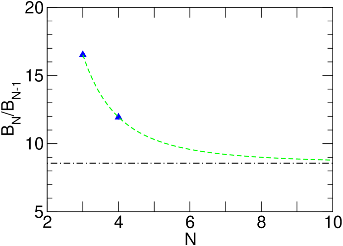
Figure 1: $B_{N}/B_{N-1}$ as a function of $N$. The dot-dashed line shows the asymptotic value of $8.567$. The dashed line is an estimate of how the large-$N$ value is approached.

The dashed line gives an estimate of how the large-$N$ value should be approached. This estimate assumes the expansion:

$$B_{N}=\left(c_{0}+\frac{c_{-1}}{N}+\frac{c_{-2}}{N^{2}}+\ldots\right)\,8.567^{N}\,,$$ (13)

leading to

$$\frac{B_{N}}{B_{N-1}}=8.567+{\cal O}\left(N^{-2}\right)\,.$$ (14)

The dashed line in Fig. 1 was obtained by fitting the coefficients of the $1/N$ and $1/N^{2}$ terms in Eq. (14) to the data points for $N=3,4$. A scenario where the corrections to Eq. (14) already start at ${\cal O}(N^{-1})$ is disfavored by the data points in Fig. 1.

Summary & Conclusion.—We have computed the four-body binding energies of weakly attractive bosons with a shallow two-body bound state in 2D. We found exactly two bound states and obtained the values $B_{4}^{(0)}=197.3(1)\,B_{2}$ for the ground state and $B_{4}^{(1)}=25.5(1)\,B_{2}$ for the excited state. The four-body system is considerably closer to the universal large-$N$ result ${B_{N}}/{B_{N-1}}=8.567$ derived in Ref. [5] than the three-body system.

It would be important to test this prediction at even larger $N$ both theoretically and experimentally. Exact solutions of the quantum-mechanical $N$-body equations, however, are currently not feasible for $N\geq 5$. It would be interesting to see whether Monte Carlo methods such as the combined Monte Carlo/hyperspherical approach used for 3D ⁴He clusters in Ref. [15] can be adapted to this problem. This will not be an easy task, since the calculations for generic finite range potentials [12, 13, 14] are not close to the universal zero-range limit. Finally, it would be valuable to create bosonic $N$-body clusters in experiments and measure their size and binding energy. The possibility of creating such clusters in anisotropic atom traps should be investigated in the future.

We thank D. Blume, D.T. Son, and A. Nogga for discussions. This work was supported by the German Academic Exchange Service (DAAD) and the U.S. department of energy under grant DE-FG02-00ER41132.

References

- [1] Safonov, A. I., Vasilyev, S. A., Yasnikov, I. S., Lukashevich, I. I., Jaakkola, S.: Phys. Rev. Lett. 81, 4545 (1998)
- [2] Görlitz, A. et al.: Phys. Rev. Lett. 87, 130402 (2001)
- [3] Schreck, F. et al.: Phys. Rev. Lett. 87, 080403 (2001)
- [4] Rychtarik,D. , Engeser, B., Nägerl, H.-C., Grimm, R.: Phys. Rev. Lett. 92, 173003 (2004)
- [5] Hammer, H.-W., Son, D. T.: arXiv:cond-mat/0405206
- [6] Pandharipande, V. R., Zabolitzky, J. G., Pieper, S. C., Wiringa, R. B., Helmbrecht, U.: Phys. Rev. Lett. 50, 1676 (1983)
- [7] Bruch, L. W., Tjon, J. A.: Phys. Rev. A 19, 425 (1979)
- [8] Nielsen, E., Fedorov, D. V., Jensen, A. S.: Few-Body Syst. 27, 15 (1999)
- [9] Platter, L., Hammer, H. W., Meißner, U.-G.: arXiv:cond-mat/0404313
- [10] Yakubovsky, O. A.: Sov. J. Nucl. Phys. 5, 937 (1967) [Yad. Fiz. 5, 1312 (1967)]
- [11] Glöckle, W., Kamada, H.: Nucl. Phys. A 560, 541 (1993)
- [12] Tjon, J. A.: Phys. Rev. A 21, 1334 (1980)
- [13] Lim, T. K., Nakaichi, S., Akaishi, Y., Tanaka, H.: Phys. Rev. A 22, 28 (1980)
- [14] Vranjes, L., Kilić, S.: Phys. Rev. A 65, 042506 (2002)
- [15] Blume, D., Greene, C. H.: J. Chem. Phys. 112, 8053 (2000)