Fractionation effects in phase equilibria of polydisperse hard sphere colloids

Abstract

The equilibrium phase behaviour of hard spheres with size polydispersity is studied theoretically. We solve numerically the exact phase equilibrium equations that result from accurate free energy expressions for the fluid and solid phases, while accounting fully for size fractionation between coexisting phases. Fluids up to the largest polydispersities that we can study (around 14%) can phase separate by splitting off a solid with a much narrower size distribution. This shows that experimentally observed terminal polydispersities above which phase separation no longer occurs must be due to non-equilibrium effects. We find no evidence of re-entrant melting; instead, sufficiently compressed solids phase separate into two or more solid phases. Under appropriate conditions, coexistence of multiple solids with a fluid phase is also predicted. The solids have smaller polydispersities than the parent phase as expected, while the reverse is true for the fluid phase, which contains predominantly smaller particles but also residual amounts of the larger ones. The properties of the coexisting phases are studied in detail; mean diameter, polydispersity and volume fraction of the phases all reveal marked fractionation. We also propose a method for constructing quantities that optimally distinguish between the coexisting phases, using Principal Component Analysis in the space of density distributions. We conclude by comparing our predictions to perturbative theories for near-monodisperse systems and to Monte Carlo simulations at imposed chemical potential distribution, and find excellent agreement.

I Introduction

I.1 The hard sphere model

Hard spheres are particles that do not interact except via an infinite repulsion on contact. In a hard sphere system there is no contribution to the internal energy, $U$, from interparticle forces since $U$ is zero for all the allowed configurations. Minimising the free energy, $F=U-TS$, is thus equivalent to maximising the entropy, $S$: the structure and phase behaviour of hard spheres is determined solely by entropy. Temperature $T$ only features as a trivial factor setting the energy scale.

The hard sphere model was originally introduced as a mathematically simple model of atomic liquids (see e.g. HanMcD86 ), but has since also been recognised as a useful basic model for complex fluids RusSavSch89 such as spherical colloids. Colloidal particles coated with a thin polymeric layer so that strong steric repulsions dominate the attractive dispersion forces between the colloidal cores behave in many ways as hard spheres. Indeed, crystallisation can be observed at densities similar to those predicted by computer simulation for hard spheres, with a single-phase fluid below volume fractions $\phi\approx 0.494$, fluid-solid coexistence at up to $\phi\approx 0.545$, and a single-phase solid at higher volume fractions PusVan86 ; PauAck90 . Measurements of the osmotic pressure and compressibility similarly show very good agreement with predicted hard sphere properties Goetze91 .

There is, however, one important and unavoidable difference between colloids and the classical hard sphere model: whereas the spheres in the classical model are identically sized, colloidal particles have an inevitable spread of diameters. The magnitude of this spread is conveniently characterised by the parameter $\delta$, which is often also referred to as polydispersity and measures the standard deviation of the diameter distribution normalised by its mean:

$$\delta=\frac{\left(\overline{\sigma^{2}}-\overline{\sigma}^{2}\right)^{\frac{1}{2}}}{\overline{\sigma}}\;.$$ (1)

Here the averages $\overline{\sigma}$ and $\overline{\sigma^{2}}$ are defined via

$$\rho_{i}\equiv\rho\overline{\sigma^{i}}=\int d\sigma\rho(\sigma)\sigma^{i}\;,$$ (2)

with $\rho(\sigma)$ the density distribution of the system. The latter is defined so that the number density of particles with diameter between $\sigma$ and $\sigma+d\sigma$ is given by $\rho(\sigma)\;d\sigma$. The total density is then $\rho=\int d\sigma\rho(\sigma)$, and $n(\sigma)=\rho(\sigma)/\rho$ is the normalised diameter distribution. The $\rho_{i}$ are the moments of the density distribution, with $\rho_{0}\equiv\rho$. The presence of polydispersity in the system brings in a new parameter that allows us to distinguish between size distributions of different widths; the shape of the diameter distribution is of course also relevant. Compared to the monodisperse case, polydispersity causes several qualitatively new phenomena which have received much interest in recent years.

I.2 New phenomena arising from polydispersity

The effect of polydispersity on the phase behaviour of hard spheres has been investigated by experiments PusVan86 ; Pusey91 , computer simulations DicPar85 ; BolKof96 ; BolKof96b ; PhaRusZhuCha98 ; KofBol99 , density functional theories BarHan86 ; McrHay88 , and simplified analytical theories Pusey87 ; PhaRusZhuCha98 ; Bartlett97 ; Bartlett98 ; Sear98 ; BarWar99 ; XuBau03 ; Sollich02 . We will now outline the main findings and introduce the relevant terminology.

First, it is intuitively clear Pusey87 that significant diameter polydispersity should destabilize the crystal phase, because it is difficult to accommodate a range of diameters in a lattice structure. Experiments have indeed shown that crystallisation is suppressed above a terminal polydispersity of $\delta_{\rm t}\approx 0.12$ PusVan86 ; Pusey91 . Since then much theoretical work has focused on estimating $\delta_{\rm t}$. Dickinson et al DicPar85 , for example, extrapolated the decrease of the volume change on melting with polydispersity to zero, obtaining an estimate of $\delta_{\rm t}\approx 0.12$. Pusey Pusey87 used a simple Lindemann-type criterion to estimate that the larger spheres in a polydisperse system would disrupt the crystal structure above $\delta_{\rm t}\approx 0.06\ldots 0.12$. McRae and Haymet McrHay88 used density functional theory (DFT) and found that there was no crystallisation above $\delta_{\rm t}\approx 0.05$. Barrat and Hansen BarHan86 also employed DFT, estimating the free energy difference between fluid and solid. Taken together, this body of theoretical work suggests that the terminal polydispersity arises from a progressive narrowing of the fluid-solid coexistence region with increasing $\delta$, with phase boundaries meeting at $\delta_{\rm t}$ McrHay88 ; Bartlett97 in a point that has been identified as one of equal concentration BarWar99 (rather than a critical point).

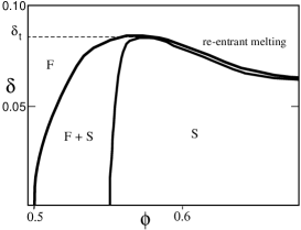
Figure 1: Sketch of the fluid (F) and solid (S) phase boundaries for polydisperse hard spheres, following BarWar99 . The boundaries are plotted as polydispersity $\delta$ versus volume fraction $\phi$. The fluid boundary approaches the solid one until they meet at a terminal polydispersity, $\delta_{\rm t}$. For $\delta$ just below $\delta_{\rm t}$, this scenario suggests re-entrant melting: compressing the crystal to sufficiently high volume fraction should transform it back into a fluid.

Bartlett and Warren BarWar99 also found re-entrant melting on the high-density side of this point: for $\delta$ just below $\delta_{\rm t}$, they predicted that compressing a crystal could transform it back into a fluid. Fig. 1 shows a sketch of this scenario.

Physically, the existence of re-entrant melting would suggest that, while in the monodisperse case the solid has the lower free energy at all volume fractions above $\phi\approx 55$%, the fluid can become preferred again at large $\phi$ if the polydispersity is sufficiently large. This result is compatible with the intuition that polydispersity reduces the maximum packing fraction in a crystal (since a range of diameters need to be accommodated on uniformly spaced lattice sites), while it increases the maximum packing fraction in the fluid, where smaller spheres should be able to fill “holes” between larger particles more easily.

This intuition can be made more quantitative by comparing the fluid and solid free energies, following Bartlett00 . The basic analysis by Bartlett and Warren BarWar99 ignores fractionation, i.e. the fact that coexisting phases need not have identical diameter distributions as long as they combine to give the correct overall or “parent” distribution $\rho^{(0)}(\sigma)$. The normalised diameter distribution is thus fixed and equal in all phases. In the moment free energy (MFE) method described below this corresponds to retaining only the overall density $\rho_{0}$. Phase equilibria can then be found by the usual double-tangent construction Sollich02 from a plot of the (moment) free energy density $f$ versus $\rho_{0}$. We display such free energy plots in Fig. 2, showing along the $x$-axis the volume fraction $\phi$ rather than $\rho_{0}$; the two are proportional for fixed diameter distribution. (The free energies are those also used for our detailed calculations below. The diameter distribution was of a Schultz form, but other size distributions are expected to give similar results.) For polydispersities up to $\delta=0.08$ a tangent plane between the solid and fluid phases always exists, giving the conventional fluid-solid coexistence. At $\delta=0.08$, re-entrant melting has appeared: a second double tangent is possible because at large volume fractions the solid free energy is now higher than that of the fluid. As $\delta$ increases, the solid free energy continues to increase relative to the fluid and eventually lies above the latter for all $\phi$ (see $\delta=0.09$ and 0.1 in Fig. 2). The point where this first happens gives the terminal polydispersity $\delta_{\rm t}$; in our example $\delta_{\rm t}\approx 0.083$. As $\delta$ approaches $\delta_{\rm t}$ from below, the widths of both the ordinary and the re-entrant fluid-solid coexistence regions shrink to zero and merge into the point of equal concentration, consistent with the phase diagram shown in Fig. 1.

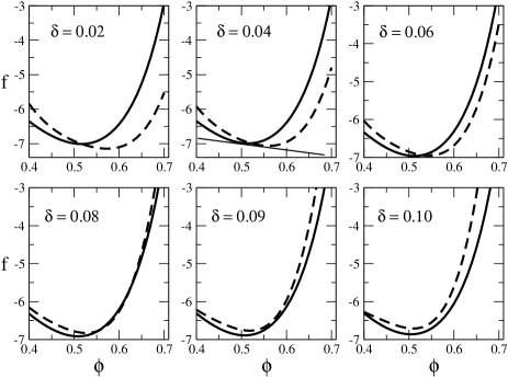
Figure 2: Free energy $f$ versus $\phi$ within the “no fractionation” approximation used by Bartlett and Warren BarWar99 . Phase separation occurs where double tangents between the fluid (thick line) and solid (dashed line) branches of the free energy can be drawn; the plot at $\delta=0.04$ shows an example (thin line). At $\delta=0.08$ re-entrant melting can be observed: two double tangents can now be drawn. For larger $\delta$, phase separation is no longer predicted. (A linear term $-19\phi$ has been added to all free energies to make the plots more readable.)

As mentioned above, this picture ignores the possibility of fractionation. Bartlett and Warren BarWar99 investigated fractionation effects approximately, by using a MFE with two density variables included, $\rho_{0}$ and $\rho_{1}=\rho\bar{\sigma}$. They concluded that the phase diagram topology remained qualitatively unchanged; quantitatively, the point of equal concentration was shifted to higher density and lower polydispersity. It has to be born in mind, however, that while the approach of BarWar99 allowed coexisting phases to have different mean diameters, it implicitly still constrained them to have the same $\delta$. (This is because, within the MFE method applied to the Schultz prior $R(\sigma)\propto\sigma^{z}e^{-(z+1)\sigma}$ of BarWar99 , the density distributions $\rho(\sigma)=R(\sigma)e^{\lambda_{0}+\lambda_{1}\sigma}\propto\sigma^{z}e^{[\lambda_{1}-(z+1)]\sigma}$ in all phases are also Schultz, with common $z$ and therefore common $\delta=(1+z)^{-1/2}$.) On the other hand, numerical simulations that allow for fractionation show that a solid with a narrow size distribution can coexist with an essentially arbitrarily polydisperse fluid BolKof96 ; BolKof96b ; KofBol99 . This suggests that the prediction of re-entrant melting should be re-examined theoretically, allowing for such fractionation effects. Conceptually, it also implies that the concept of a terminal polydispersity is likely to be useful only for the solid but not for the fluid, and we will see this confirmed below.

Fractionation has also been predicted to lead to solid-solid coexistence Bartlett98 ; Sear98 ; Bartlett00 , where a broad diameter distribution is split into a number of narrower solid fractions. This occurs because the loss of entropy of mixing is outweighed by the better packing, and therefore higher entropy, of crystals with narrow size distribution; accordingly, as the overall polydispersity of the system grows, the number of coexisting solids is predicted to increase. Fig. 3 sketches this effect, following the treatment of Bartlett98 . There is no coexistence region between fluid and solid, due to a simplification in the analysis of Bartlett98 : rather than solving the phase equilibrium conditions, only the free energies were equated between the fluid and the (one or several) solid phases. The resulting lines in the phase diagram generally lie inside the actual phase separation region, but give a rough guide to the phase transitions that can occur. The parent diameter distribution considered had a “top hat” form (uniform between given minimum and maximum diameters), and for multiple solids fractionation was assumed to be “hard”, with the parent distribution split into non-overlapping top hat distributions with identical polydispersities.

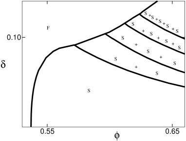
Figure 3: Sketch of fluid (F) and multiple solid (S) phase coexistences in polydisperse hard spheres, following Bartlett98 . Approximate phase boundaries are plotted as polydispersity $\delta$ versus volume fraction $\phi$. For sufficiently large $\delta$ and $\phi$, coexistence of several solids is predicted; see text for discussion.

Previous work as described above leaves open a number of questions. The rather drastic, and differing, approximations for size fractionation used in previous studies of re-entrant melting and solid-solid coexistence BarWar99 ; Bartlett98 ; Sear98 ; Bartlett00 , as described above, leave the relative importance of these two phenomena unclear. Theoretical calculations that account fully for fractionation remain restricted to highly simplified van der Waals free energies XuBau03 . Numerical simulations can in principle also capture arbitrary fractionation behaviour, but have been carried out at constant chemical potential distribution BolKof96 ; BolKof96b ; KofBol99 . As explained in more detail in Section VI.2, the system’s overall particle size distribution can then change dramatically across the phase diagram. This is in contrast to the experimental situation and so limits the applicability of the results.

Our main aim in this study is, therefore, to calculate the equilibrium phase behaviour of polydisperse hard spheres on the basis of accurate free energy expressions, taking full account of fractionation and going beyond previous work on fluid-solid and solid-solid coexistence. The experimentally observed behaviour of hard sphere colloids will of course also depend on non-equilibrium effects, e.g. the presence of a kinetic glass transition PusVan87 , anomalously large nucleation barriers AueFre01 or the growth kinetics of polydisperse crystals EvaHol01 . Nevertheless, the equilibrium phase behaviour needs to be understood as a baseline from which non-equilibrium effects can be properly attributed. Also, more of the equilibrium behaviour may be observable under microgravity conditions, where the glass transition is shifted to higher densities or even absent ZhuLiRogMeyOttRusCha97 .

We begin in Section II by defining the free energies we use to describe the fluid and solid phases of polydisperse hard spheres. Section III reviews the moment free energy method and its numerical implementation for solving the phase equilibrium conditions. In Section IV we then describe the basic features of the phase behaviour that we find; a short account of these results has appeared in FasSol03 . Section V describes in detail the fractionation effects that we predict, and introduces a new method for constructing optimal visualisations of polydisperse phase behaviour. Section VI, finally, compares our results to perturbative theories for the near-monodisperse limit and to Monte Carlo simulations at constant chemical potential differences. The agreement is very good, thus validating our approach. We conclude in Section VII with a summary and outlook towards future work.

II Free energies

Our starting point is the decomposition of the free energy of a polydisperse system into an ideal and an excess part,

$$f=\int d\sigma\rho(\sigma)\left[\ln\rho(\sigma)-1\right]+f^{\rm ex}(\{\rho_{i}\})$$ (3)

The excess part $f^{\rm ex}$ can, in principle, depend on all details of $\rho(\sigma)$ and therefore on all of its moments $\rho_{i}$, but we will be concerned with truncatable free energies SolWarCat01 . For these, the dependence is only through a finite number of moments, for us specifically $\rho_{0},\ldots,\rho_{3}$.

Strictly speaking, equation (3) gives the free energy density; we will continue to refer to this as the free energy for short. Also, all quantities in (3) are dimensionless: we assume that sphere diameters are measured in units of some reference value $\sigma_{0}$, that all densities are made dimensionless by multiplying by the volume $v_{0}=\pi\sigma_{0}^{3}/6$ of a reference sphere, and that all energies are measured in units of $T=1/\beta$. Boltzman’s constant $k_{\rm B}$ is set to 1 throughout. Free energy and pressure are then in units of $T/v_{0}$, for example. Table 1 summarises the relations between important dimensionless and dimensional quantities. Conveniently, with our choice of units $\rho_{3}\equiv\phi$ is simply the volume fraction of spheres.

Dimensionless		Dimensional
$\sigma$	=	$\tilde{\sigma}/\sigma_{0}$
$f$	=	$\beta v_{0}\tilde{f}$
$P$	=	$\beta v_{0}\tilde{P}$
$\rho(\sigma)$	=	$v_{0}\sigma_{0}\tilde{\rho}(\tilde{\sigma})$
$\rho_{i}$	=	$({v_{0}}/{\sigma_{0}^{i}})\tilde{\rho}_{i}$
$\mu^{\rm ex}(\sigma)$	=	$\beta\tilde{\mu}^{\rm ex}(\tilde{\sigma})$
$\mu^{\rm ex}_{i}$	=	$\sigma_{0}^{i}\tilde{\mu}_{i}^{\rm ex}$

Table 1: Relations between dimensional and dimensionless quantities. All dimensional quantities except for the units $\beta$, $\sigma_{0}$ and $v_{0}$ themselves are denoted by tildes “$\sim$”.

For the fluid phase of polydisperse hard spheres, the most accurate free energy approximation available is the generalisation by Salacuse and Stell SalSte82 of the equation of state due to Boublik, Mansoori, Carnahan, Starling and Leland (BMCSL) Boublik70 ; ManCarStaLel71 ; for the monodisperse case this reproduces the Carnahan-Starling equation of state CarSta69 . In our dimensionless quantities, the BMCSL expression for the excess free energy takes the form

$$f^{\rm ex}=\left(\frac{\rho_{2}^{3}}{\rho_{3}^{2}}-\rho_{0}\right)\ln(1-\rho_{3})+\frac{3\rho_{1}\rho_{2}}{1-\rho_{3}}+\frac{\rho_{2}^{3}}{\rho_{3}(1-\rho_{3})^{2}}$$ (4)

As anticipated above, this is truncatable, involving only the moments $\rho_{i}=\int d\sigma\rho(\sigma)\sigma^{i}$ ($i=0\ldots 3$) of the density distribution. Bartlett Bartlett99 provided an elegant argument why—at least within a virial expansion—such a moment structure of the excess free energy for the hard sphere fluid should in fact be exact.

For phase coexistence calculations we will also need to have a compact expression for the excess free energy of the polydisperse hard sphere crystal. This is not at all a trivial question. In principle, the structure of a polydisperse crystal could be rather complex, with different sites inside the crystalline unit cell occupied preferentially by particles with different ranges of diameters. The system would then effectively be an ordered solid solution (see e.g. CotParVegMon96 ; CotMon95 ). Most theoretical work makes the simplifying assumption that one has a substitutionally disordered solid, where crystal sites are assumed to be occupied equally likely by particles of any diameter (see e.g. BarBauHan86 ; KraFre91 ).

A simple-minded but popular approach to estimating the free energy is cell theory, first introduced by Kirkwood kirkwood50 and widely used since (see e.g. Sear98 ): particles are treated as independent but confined to an effective cell formed by their neighbours. However, it is clear that for a polydisperse system this is unlikely to be a useful approximation. For example, the cells of the model would have to be made large enough to accommodate the particles with the largest diameter, even if the fraction of such particles is very small.

We follow instead the more quantitative, “geometric” approach proposed by Bartlett Bartlett99 ; Bartlett97 . He assumed that the excess free energy of the solid depends on the same moments $\rho_{0},\ldots,\rho_{3}$ as that of the fluid. This can be motivated from scaled particle theory ReiFriLeb59 ; LebHelPar65 , which suggests that the excess chemical potential, $\mu^{\rm ex}(\sigma)$, of spheres of diameter $\sigma$ is given by a cubic polynomial in $\sigma$

$$\mu^{\rm ex}(\sigma)=\mu_{0}^{\rm ex}+\mu_{1}^{\rm ex}\sigma+\mu_{2}^{\rm ex}\sigma^{2}+\mu_{3}^{\rm ex}\sigma^{3}$$ (5)

The coefficients $\mu_{0}^{\rm ex}$ and $\mu_{3}^{\rm ex}$ can be determined from the Widom insertion principle Widom63 . The latter can be stated as saying that $\exp(-\mu^{\rm ex}(\sigma))$ is the ratio of the (excess parts of the) partition functions for $N+1$ and $N$ particles, where the added particle has diameter $\sigma$. (Equivalently the excess chemical potential may be interpreted as the work of inserting an $(N+1)$-th hard sphere of diameter $\sigma$ into a system of $N$ spheres.) In a system with purely hard interactions, this implies that $\mu^{\rm ex}(\sigma)$ is positive and an increasing function of $\sigma$. For large $\sigma$, the presence of the added particle effectively just reduces the volume available to the $N$ others, giving $\mu^{\rm ex}(\sigma)\approx P\sigma^{3}$ ($=\tilde{P}(\pi/6)\tilde{\sigma}^{3}$ in dimensional units), hence $\mu_{3}^{\rm ex}=P$. For small $\sigma$, one notes that the ratio of the (excess) partition functions is also the average Boltzmann factor of the added particle, the average being over the Boltzmann distribution of the $N$-particle system. In the hard sphere case, $\exp(-\mu^{\rm ex}(\sigma))$ is thus the probability of being able to insert a particle without overlap. In the limit of vanishing particle this probability is $1-\phi$, giving $\mu^{\rm ex}(\sigma\to 0)=\mu_{0}^{\rm ex}=-\ln(1-\phi)$.

One now notes that (5) implies that the excess free energy can only depend on the moments $\rho_{0},\ldots,\rho_{3}$. Indeed, from the definition of the excess chemical potentials and with the dependence of the excess free energy on $\rho(\sigma)$ expressed through a (possibly infinite) set of moments $\rho_{i}$,

$$\mu^{\rm ex}(\sigma)=\frac{\delta f^{\rm ex}}{\delta\rho(\sigma)}=\sum_{i}\mu^{\rm ex}_{i}\sigma^{i},\qquad\mu^{\rm ex}_{i}=\frac{\partial f^{\rm ex}}{\partial\rho_{i}}$$

A comparison with the form (5) of the excess chemical potentials reveals that $f^{\rm ex}$ can only depend on $\rho_{0},\ldots,\rho_{3}$, as claimed. The same is then true also for the $\mu^{\rm ex}_{i}=\partial f^{\rm ex}/\partial\rho_{i}$ ($i=0,\ldots,3$), which are recognised as excess moment chemical potentials. The excess free energy of a polydisperse hard sphere mixture can thus be deduced from that of any other mixture which is equivalent in the sense of having the same $\rho_{0},\ldots,\rho_{3}$. These moments determine the number density along with the basic geometric properties of mean particle diameter, surface area and volume. The simplest mixture with a finite number of species that can match any given $\rho_{0},\ldots,\rho_{3}$ is a bidisperse one. Indeed, this has four degrees of freedom, namely, the number densities and particle diameters of the two species. We can therefore identify the excess free energy of a polydisperse hard sphere solid with that of the equivalent bidisperse system. For the latter, we follow Bartlett in using the fits to the simulation data of Kranendonk et al KraFre91 . Because these data are obtained for an fcc substitutionally disordered crystal, an implicit assumption is that the polydisperse crystal will have the same structure.

There is a difficulty in Bartlett’s approach with the determination of the excess moment chemical potentials $\mu_{0}^{\rm ex},\ldots,\mu_{3}^{\rm ex}$. He fixed $\mu_{0}^{\rm ex}$ and $\mu_{3}^{\rm ex}$ to the exact results derived from the Widom insertion principle, $\mu_{0}^{\rm ex}=-\ln(1-\rho_{3})$ and $\mu_{3}^{\rm ex}=P$. The remaining two excess moment chemical potentials, $\mu_{1}^{\rm ex}$ and $\mu_{2}^{\rm ex}$, can then be found from the bidisperse simulation data, by requiring $\mu^{\rm ex}(\sigma)$ at the diameters of the small and large spheres to agree with the simulated excess chemical potentials of the two species. However, because of the approximate character of the excess free energy, the $\mu^{\rm ex}(\sigma)$ derived by this route do not obey the thermodynamic consistency requirement $\delta\mu^{\rm ex}(\sigma)/\delta\rho(\sigma^{\prime})=\delta\mu^{\rm ex}(\sigma^{\prime})/\delta\rho(\sigma)$, which corresponds to $\partial\mu_{i}^{\rm ex}/\partial\rho_{j}=\partial\mu_{j}^{\rm ex}/\partial\rho_{i}$ for the excess moment chemical potentials. To avoid this in our study, we assign the latter by explicitly evaluating the derivatives of the excess free energy, $\mu^{\rm ex}_{i}=\partial f^{\rm ex}/\partial\rho_{i}$. Thermodynamic consistency is then automatic. The price we pay is that our $\mu^{\rm ex}(\sigma)$ no longer has the theoretically expected asymptotic behaviour for $\sigma\to 0$ and $\sigma\to\infty$. This means that we have to restrict use of our solid free energy to relatively narrow diameter distributions, as discussed in more detail below.

III Numerical method

III.1 Moment free energy

Our computational approach for determining the phase behaviour of polydisperse hard spheres is based on the moment free energy (MFE) method. We give a brief outline here; details can be found in SolWarCat01 ; Warren98 ; SolCat98 ; Sollich02 . Recall first the phase equilibrium conditions for coexistence of $p$ phases, in a system described by a truncatable free energy. By definition, the excess free energy then depends on a finite set of $M$ (generalised) moments $\rho_{i}=\int\!d\sigma\,\rho(\sigma)w_{i}(\sigma)$ defined by weight functions $w_{i}(\sigma)$; above we had $w_{i}(\sigma)=\sigma^{i}$. In coexisting phases, the chemical potentials $\mu(\sigma)$ and pressure $P$ must be equal. The former are, by differentiation of (3),

$$\mu(\sigma)=\frac{\delta f}{\delta\rho(\sigma)}=\ln\rho(\sigma)+\sum_{i}\mu^{\rm ex}_{i}w_{i}(\sigma)$$ (6)

with $\mu^{\rm ex}_{i}={\partial f^{\rm ex}}/{\partial\rho_{i}}$ as before. The pressure is given by the Gibbs-Duhem relation

$$P=-f+\int\!d\sigma\,\mu(\sigma)\rho(\sigma)=\rho_{0}-f^{\rm ex}+\sum_{i}\mu^{\rm ex}_{i}\rho_{i}$$ (7)

To the conditions of equality of chemical potentials and pressure we need to add the requirement of conservation of particle number for each species $\sigma$, which reads

$$\sum_{\alpha}v^{(\alpha)}\rho^{(\alpha)}(\sigma)=\rho^{(0)}(\sigma)$$ (8)

where $\alpha=1,\ldots,p$ labels the phases and $v^{(\alpha)}$ is the fraction of the system volume occupied by phase $\alpha$. One then finds from equality of the $\mu(\sigma)$, Eq. (6), together with particle conservation (8), that the density distributions in coexisting phases can be written as

$$\rho^{(\alpha)}(\sigma)=\rho^{(0)}(\sigma)\,\frac{\exp\left[\sum_{i}\lambda_{i}^{(\alpha)}w_{i}(\sigma)\right]}{\sum_{\gamma}v^{(\gamma)}\exp\left[\sum_{i}\lambda_{i}^{(\gamma)}w_{i}(\sigma)\right]}$$ (9)

Here the $\lambda_{i}^{(\alpha)}$ must obey

$$\lambda_{i}^{(\alpha)}=-\mu_{i}^{(\alpha),{\rm ex}}+c_{i}$$ (10)

and the $c_{i}$ are undetermined constants that do not affect the density distributions (9). One can fix them e.g. by requiring all the $\lambda_{i}^{(\alpha)}$ in one of the phases to be zero. A little reflection then shows that (10) together with $\sum_{\alpha}v^{(\alpha)}=1$ and the equality of the pressures (7) in all phases give a closed system of nonlinear equations for the $p(M+1)$ variables $\lambda_{i}^{(\alpha)}$ and $v^{(\alpha)}$. A solution can thus, in principle, be found by a standard algorithm such as Newton-Raphson. Generating an initial point from which such an algorithm will converge, however, is still a nontrivial problem, especially when more than two phases coexist and/or many moments $\rho_{i}$ are involved. Furthermore, the nonlinear phase equilibrium equations permit no simple geometrical interpretation or qualitative insight akin to the construction of phase diagrams from the free energy surface of a finite mixture.

The moment free energy addresses these two disadvantages. To construct it, one starts by modifying the free energy decomposition (3) to

$$f=\int\!d\sigma\,\rho(\sigma)\left[\ln\frac{\rho(\sigma)}{R(\sigma)}-1\right]+f^{\rm ex}(\{\rho_{i}\})$$ (11)

In the first (ideal) term, a normalising factor $R(\sigma)$ has been included inside the logarithm. This has no effect on the exact thermodynamics because it contributes only terms linear in $\rho(\sigma)$, but will play a central role below. One can now argue that the most important moments to treat correctly in the calculation of phase equilibria are those that actually appear in the excess free energy $f^{\rm ex}(\{\rho_{i}\})$. Accordingly, one imposes particle conservation (8) only for the $\rho_{i}$, but allows it to be violated in other details of the density distribution $\rho(\sigma)$ which do not affect the $\rho_{i}$. These “transverse” degrees of freedom are instead chosen to minimise the free energy (11), and more precisely its ideal part since the excess contribution is a constant for fixed values of the $\rho_{i}$. This minimisation gives

$$\rho(\sigma)=R(\sigma)\exp\left[\sum_{i}\lambda_{i}w_{i}(\sigma)\right]$$ (12)

where the Lagrange multipliers $\lambda_{i}$ are chosen to give the desired values of the moments

$$\rho_{i}=\int\!d\sigma\,w_{i}(\sigma)\,R(\sigma)\exp\left[\sum_{j}\lambda_{j}w_{j}(\sigma)\right]$$ (13)

The corresponding minimum value of $f$ as given in (11) then defines the moment free energy (MFE)

$$f_{\rm mom}(\{\rho_{i}\})=\left(\sum_{i}\lambda_{i}\rho_{i}-\rho_{0}\right)+f^{\rm ex}(\{\rho_{i}\})$$ (14)

Since the Lagrange multipliers are (at least implicitly) functions of the moments $\rho_{i}$, the MFE depends only on the $\rho_{i}$. These can now be viewed as densities of “quasi-species” of particles, allowing for example the calculation of moment chemical potentials SolWarCat01

$$\mu_{i}=\frac{\partial f_{\rm mom}}{\partial\rho_{i}}=\lambda_{i}+\frac{\partial f^{\rm ex}}{\partial\rho_{i}}=\lambda_{i}+\mu^{\rm ex}_{i}$$ (15)

and the corresponding pressure $P=\sum_{i}\mu_{i}\rho_{i}-f_{\rm mom}$ which turns out to be identical to the exact expression (7). A finite-dimensional phase diagram can thus be constructed from $f_{\rm mom}$ according to the usual tangency plane rules, ignoring the underlying polydisperse nature of the system. Obviously, though, the results now depend on $R(\sigma)$. To understand its influence, one notes that the MFE is simply the free energy of phases in which the density distributions $\rho(\sigma)$ are of the form (12). To ensure that the parent phase is contained in the family, one normally chooses its density distribution as the prior, $R(\sigma)=\rho^{(0)}(\sigma)$; the MFE procedure will then be exactly valid whenever the density distributions actually arising in the various coexisting phases are members of the corresponding family

$$\rho(\sigma)=\rho^{(0)}(\sigma)\exp\left[\sum_{i}\lambda_{i}w_{i}(\sigma)\right]$$ (16)

It is easy to show from (9) that this condition holds whenever all but one of a set of coexisting phases are of infinitesimal volume compared to the majority phase. Accordingly, the MFE yields exactly the onset of phase of coexistence, conventionally represented via cloud and shadow curves (see below). Similarly, one can show that spinodals and critical points are found exactly SolWarCat01 .

For coexistences involving finite amounts of different phases the MFE only gives approximate results, since different density distributions from the family (16), corresponding to two (or more) phases arising from the same parent $\rho^{(0)}(\sigma)$, do not in general add to recover the parent distribution itself. Moreover, from Gibbs’ phase rule, a MFE depending on $M$ moments will not predict more than $M+1$ coexisting phases, while we know that a polydisperse system can in principle separate into an arbitrary number of phases. Both of these shortcomings can be overcome by including extra moments within the MFE. By choosing the weight functions of the extra moments adaptively, the properties of the coexisting phases can then be predicted with in principle arbitrary accuracy ClaCueSeaSolSpe00 ; SolWarCat01 . Importantly for us, the results can in fact be used as initial points from which a solution of the exact phase equilibrium problem can be converged successfully SpeSol02 ; SpeSol03a . This is the technique that we use here. Once a phase split for a given parent distribution $\rho^{(0)}(\sigma)$ has been found, care needs to be taken to check that it is globally stable, i.e. that no phase split of lower free energy exists SolWarCat01 . Adopting this procedure, we are able to calculate coexistence of up to five phases, which so far has been possible only for much simpler free energies depending on a single density moment (see e.g. SolWarCat01 ).

III.2 Implementation

We focus below on parent distributions with unit mean particle diameter $\overline{\sigma}$; any other choice could be absorbed into the unit length $\sigma_{0}$. For small polydispersity $\delta$, the standard moments $\rho_{i}=\int\!d\sigma\,\rho(\sigma)\sigma^{i}$ then become very close to each other, and in fact strictly identical in the limit $\delta\to 0$. This causes numerical difficulties, and we therefore work instead with the centred moments $\rho^{\rm c}_{i}=\int\!d\sigma\,\rho(\sigma)[(\sigma-1)/\delta_{0}]^{i}$ which remain distinct even for small $\delta$. The factor $\delta_{0}$ is included to ensure that the moments are all of comparable magnitude. We therefore choose it in the middle of the range of polydispersities $\delta$ that we study, with typically $\delta_{0}=0.05$. The centred moments are obviously linearly related to the conventional ones, e.g. $\rho^{\rm c}_{1}=(\rho_{1}-\rho_{0})/\delta_{0}$. The BMCSL and solid free energies can therefore readily be re-expressed in term of the centred moments. Because the transformation between the two sets of moments is linear, the corresponding sets of excess moment chemical potentials $\mu^{\rm ex}_{i}=\partial f^{\rm ex}/\partial\rho_{i}$ are also linearly related and easily converted into each other.

We combine the fluid and solid branches of our excess free energy by simply taking the minimum for a given set of moments. Some care is needed here: because the solid free energy is derived from fits to simulation data for bidisperse systems (see above ), we expect it to be reliable only in the region spanned by the simulations KraFre91 . The smallest diameter ratio investigated in the simulations is $\alpha=0.85$. The maximum polydispersity that can be reached in a bidisperse system for this diameter ratio is $\delta=(\alpha+1/\alpha-2)^{1/2}/2\approx 0.08$. We therefore restrict use of the solid free energy to phases with polydispersity below this value. Reassuringly, we will see below that all solid phases occurring in equilibrium phase splits are well below this threshold.

A further constraint on the use of the solid free energy arises from the fact that, as explained above, our excess chemical potentials $\mu^{\rm ex}(\sigma)$ do not have the correct limiting behaviour predicted from the Widom insertion principle for $\sigma\to 0$ and $\sigma\to\infty$. Physically, this is again plausible because we are extrapolating to sphere diameters far from the mean of the distribution, and therefore far from the regime where the simulation data will be reliable. We will therefore always work with diameter distributions with hard cutoffs either side of the mean so that the behaviour of $\mu^{\rm ex}(\sigma)$ for very small or large $\sigma$ never comes into play. Finally, we also restrict the volume fractions for the solid branch of the free energy to $0.494\leq\phi\leq 0.74$, which are respectively the smallest and largest $\phi$ for which monodisperse hard spheres at equilibrium exhibit a crystalline solid phase.

IV Phase behaviour

We now describe our results for the overall phase behaviour of polydisperse hard spheres. Our numerical work requires a choice to be made for the parental diameter distribution. We focus mostly on a triangular distribution, where $n^{(0)}(\sigma)=\rho^{(0)}(\sigma)/\rho_{0}^{(0)}$ is given by

$$n^{(0)}(\sigma)=\frac{1}{w^{2}}\left\{\begin{array}[]{llrcl}\sigma-(1-w)&\mbox{for}&1-w&\leq\sigma\leq&1\\ (1+w)-\sigma&\mbox{for}&1&\leq\sigma\leq&1+w\end{array}\right.$$

whose width parameter $w$ is related to the polydispersity by $w=\sqrt{6}\,\delta$. For the moderate values of $\delta$ of interest here one expects other distribution shapes to give qualitatively similar results, based on the intuition that for narrow size distributions $\delta$ is the key parameter controlling the phase behaviour Pusey87 . To verify this, we also consider briefly a Schultz parent distribution, $n^{(0)}(\sigma)\propto\sigma^{z}e^{-(z+1)\sigma}$, cut off outside the range $\sigma\in[0.8,1.2]$. For a narrow distribution, i.e. large $z$, where the cutoffs are unimportant, the polydispersity is then related to the parameter $z$ by $\delta^{2}=1/(z+1)$ and the mean diameter is unity as before.

IV.1 Onset of phase coexistence

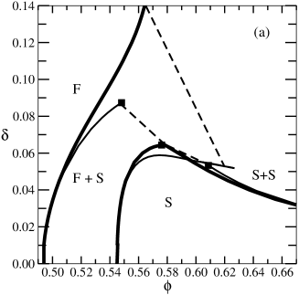
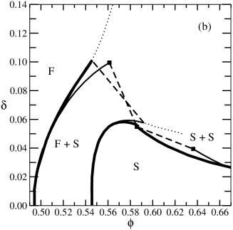
Figure 4: Cloud curves (thick) and shadow curves (thin), for polydisperse hard spheres with a triangular (a) and Schultz (b) diameter distribution. The curves show polydispersity $\delta$ versus volume fraction $\phi$ for the cloud and shadow phases; dashed lines link sample cloud-shadow pairs. The solid (S) cloud curve has two branches, with onset of F-S and S-S coexistence at low and high volume fractions, respectively. Where they meet, a triple point occurs; squares mark the cloud phase and the two coexisting shadows there. In the Schultz plot, the dotted lines indicate the expected continuations of the fluid cloud and corresponding shadow curve beyond the region where our numerical methods work reliably.

The most basic question we can ask about phase behaviour regards the onset of phase separation coming from single-phase regions. Increasing the volume fraction $\phi$ of the parent at given polydispersity $\delta$, a single-phase fluid (F) will first separate into coexisting fluid and solid (S) phases at the so-called cloud point. The locus of all cloud points in the ($\phi$,$\delta$)-plane defines the fluid cloud curve. The incipient phase corresponding to the cloud point is called the “shadow” solid; its properties define the solid shadow curve. These curves are shown in Fig. 4 (a) for a triangular parent distribution. An important feature is that the fluid cloud curve continues throughout the whole range of polydispersities that we can investigate numerically: even at $\delta=0.14$, a hard sphere fluid will eventually split off a solid on compression. This is in marked contrast to the phase diagram of BarWar99 as sketched in Fig. 1. The key difference is that our analysis accounts fully for fractionation: Fig. 4 shows that the coexisting shadow solid always has a relatively modest polydispersity, with $\delta$ never rising above $0.06$ even when the cloud fluid has $\delta=0.14$. This fractionation effect prevents the convergence of the solid and fluid phase boundaries which a theory with fixed $\delta$ BarWar99 predicts, along with the resulting re-entrant melting (Fig. 1). These findings are in qualitative accord with Monte Carlo simulations for the simpler case of fixed chemical potentials BolKof96 ; BolKof96b ; KofBol99 , discussed in detail in Section VI.2 below. The results imply, in particular, that the terminal polydispersity $\delta_{\rm t}$ cannot be defined as the point beyond which a fluid at equilibrium will no longer phase separate; $\delta_{\rm t}$ only makes sense as the maximum polydispersity at which a single solid phase can exist (see below).

The fractionation effects described above can be seen more explicitly by comparing the (normalised) diameter distributions of the fluid cloud and solid shadow phases, as displayed in Fig. 5 for (parental) polydispersity $\delta=0.05$ and $\delta=0.10$. At the cloud point the size distribution in the fluid coincides with the parent distribution as it must. The distribution in the coexisting shadow solid, on the other hand, deviates increasingly from that of the parent as the parental $\delta$ increases. In particular, the solid contains predominantly the larger particles and has a rather more narrow spread of sizes, consistent with the small solid polydispersities found above. We will see shortly that these properties are rather generic and persist inside the coexistence region.

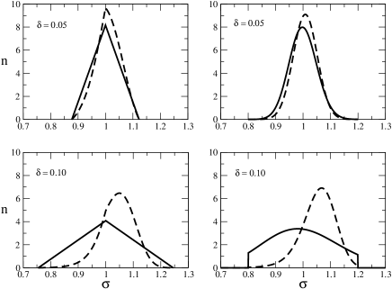
Figure 5: Normalised size distributions $n(\sigma)=\rho(\sigma)/\rho_{0}$ for the coexisting fluid and shadow phases at the fluid cloud point, for parent distributions with polydispersities $\delta=0.05$ (top) and $\delta=0.10$ (bottom) and triangular (left) and Schultz (right) shape. Solid lines show the cloud fluid, which is identical to the parent, and dashed lines the shadow solid.

We now assess the effect of the shape of the particle size distribution on these results. Fig. 4 shows that the fluid cloud and solid shadow curves are qualitatively and even quantitatively very similar for the triangular and Schultz distributions. (Numerically, we can only reach $\delta=0.10$ for the latter, but have no reason to expect that this is a physical feature and indicate the expected continuation of the curves by dotted lines.) Fig. 5 (right) demonstrates that the qualitative features of the fractionation behaviour are also the same between the two distributions, consistent with our intuition that variations in the shape of the parental size distribution have, for given $\delta$, only a minor effect.

We next consider the onset of phase separation coming from the single-phase solid, which defines the solid cloud curve and corresponding shadow curve. Initially we focus again on the triangular size distribution. Fig. 4 (a) shows that a decrease in density at low polydispersities leads to conventional fluid-solid phase separation. At higher $\delta$, however, the solid cloud curve acquires a second branch at higher densities. This is broadly analogous to the re-entrant phase boundary found in BarWar99 , but with the crucial difference that the system phase separates into two solids rather than a solid and a fluid. The two branches meet at a triple point. Here the solid cloud phase coexists with two shadow phases, one fluid and one solid, as marked by the squares in Fig. 4 (a). The triple point is located at $\delta\approx 0.07$; since it is at the maximum of both branches of the solid cloud curve, this value also gives the terminal polydispersity beyond which solids with triangular diameter distribution are unstable against phase separation.

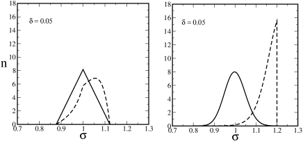
Figure 6: Normalised size distributions $n(\sigma)$ of solid cloud and shadow phases, on the high-density branch of the solid cloud curve at $\delta=0.05$. Left: triangular parent; right: Schultz parent. The solid lines show the cloud phase, the dashed lines the shadow. Note the strong size fractionation effects.

Fig. 6 (left) displays the diameter distributions for the cloud and shadow solids, at $\delta=0.05$ on the high-density branch of the solid cloud curve. In comparison with Fig. 5, what is striking is that the fractionation effects at the onset of solid-solid coexistence are much stronger than for fluid-solid phase separation at the same $\delta$. This is consistent with physical intuition. The fluid-solid phase separation exists even in the monodisperse limit. The presence of polydispersity acts as a small perturbation to this transition, certainly at low $\delta$, so that fractionation effects can be viewed as incidental. Solid-solid phase separation, on the other hand, is driven by polydispersity and could not take place without fractionation.

We compare again at this stage with the results for the Schultz parent distribution. Fig. 4 (b) shows that the cloud and shadow curves look qualitatively similar to the triangular case. Quantitatively, the low-density branch of the solid cloud curve now has a maximum, giving the terminal polydispersity as $\delta_{\rm t}\approx 0.06$. The triple point is at slightly smaller $\delta$, and the whole high-density branch of the solid cloud curve – which describes the onset of solid-solid phase separation – is shifted to smaller $\delta$ compared to the triangular parent case. Fig. 6 (right) shows the diameter distributions for the cloud and shadow solids, at the onset of phase separation at $\delta=0.05$. Compared to the triangular parent, the fractionation effects are now even stronger. In fact, the size distribution of the shadow solid continues to increase towards larger sphere diameters $\sigma$ and is terminated only by the hard cutoff at $\sigma=1.2$ which we impose in the Schultz case; note that in the cloud solid (solid line) this cutoff is hardly discernible. In the triangular case, there is no sharp cutoff effect on the shadow solid: the form of the parent forces all size distributions to drop to zero continuously at the upper end.

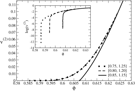
Figure 7: Fractional system volume occupied by the newly forming solid, $v^{(2)}$, versus the parent volume fraction, $\phi$, for cutoffs imposing three different ranges of particle sizes $\sigma$ as indicated in the legend. Once enough of the new solid phase exists (above $v^{(2)}\approx 0.08$) the behaviour is essentially cutoff-independent. The cloud point, on the other hand, where $v^{(2)}$ extrapolates to zero, depends strongly on the cutoff; this is more clearly visible in the linear-log plot in the inset.

The above observations for the Schultz parent suggest an analogy with recent results for isotropic-nematic phase separation in hard rod-like particles SpeSol03a ; SpeSol03b . For sufficiently wide rod length distributions, one observes there that the shadow nematic phase can become dominated by the longest rods in the system, i.e. those with lengths near the cutoff, even though these make up only a small fraction of the parent distribution. Such cutoff effects are important only near the cloud point: as soon as the new phase occupies a nonzero fraction of the overall system volume, particle conservation prevents it from containing an atypically large number of long rods. To test whether we have a similar situation for the onset of solid-solid separation from a Schultz parent, we have varied the cutoff on the sphere diameters. Fig. 7 plots the fractional system volume $v^{(2)}$ occupied by the new solid against the parent colloid volume fraction. We observe that $v^{(2)}$ is indeed cutoff-independent well inside the coexistence region, where it is non-negligible. The position of the cloud point itself, on the other hand, where $v^{(2)}$ extrapolates to zero, is strongly cutoff-dependent. We conclude, therefore, that at the onset of solid-solid coexistence from a Schultz parent with $\delta=0.05$ the shadow solid is cutoff-dominated, in analogy with the shadow nematics in the Onsager model of long hard rods SpeSol03a ; SpeSol03b .

One may wonder whether the cutoff effects described above are an artefact of the approximate nature of our excess chemical potentials for the polydisperse solid. We cannot give a definitive answer to this question here, but suggest that such effects might in fact be expected. From (6), equilibrium of chemical potentials between the cloud (parent) solid $\rho^{(0)}(\sigma)$ and the shadow solid $\rho^{(2)}(\sigma)$ implies

$$\rho^{(2)}(\sigma)=\rho^{(0)}(\sigma)\exp(-\Delta\mu^{\rm ex}(\sigma))$$ (17)

with $\mu^{\rm ex}(\sigma)=\sum_{i=0}^{3}\Delta\mu^{\rm ex}_{i}\sigma^{i}$ and $\Delta\mu^{\rm ex}_{i}$ the differences in the excess moment chemical potentials between the shadow and cloud phases. The Widom insertion principle tells us that $\mu_{3}^{\rm ex}$, being equal to the pressure, is equal in the two phases. Thus $\Delta\mu^{\rm ex}(\sigma)$ should generically be a quadratic polynomial in $\sigma$. If the $\sigma^{2}$-term has a negative coefficient, then from (17) it will overwhelm the exponential tail of the Schultz parent $\rho^{(0)}(\sigma)$. The shadow density distribution $\rho^{(2)}(\sigma)$ then increases strongly at large $\sigma$ so that its properties will be dominated by the presence of any cutoff. In fact, this argument suggests that the same could happen even with a (sufficiently polydisperse) Gaussian parent. Only a stronger decay, say $\rho^{(0)}(\sigma)\sim\exp(-\sigma^{a})$ with $a>2$, could definitely prevent cutoff effects on the shadow solid. This question deserves further study, but would require more accurate excess chemical potentials for polydisperse solids – and over a larger range of sphere diameters – than we currently have at our disposal.

So far we have investigated the global stability of single phases, i.e. the stability against macroscopic phase separation. One can also ask about local stability of the phases, i.e. the spinodal points. Since our free energy is spliced together from separate fluid and solid branches, we cannot investigate instability to fluid-solid separation. The stability of single-phase fluids against fluid-fluid demixing has been studied by Warren Warren99 and Cuesta Cuesta99 . They found, using the BMCSL free energy, that spinodal instabilities do indeed occur, but only for very broad diameter distributions such as log-normals with $\delta$ above $\approx 2.5$, or bimodal distributions with a wide size disparity between the larger and smaller spheres. At the modest values of $\delta$ that concern us here, such instabilities do not occur.

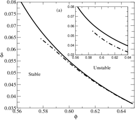
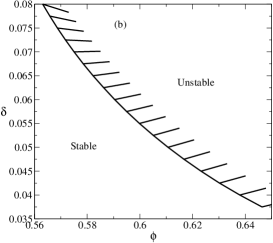
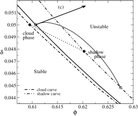
Figure 8: Spinodal instability of the polydisperse hard sphere crystal against solid-solid demixing, in the volume fraction – polydispersity plane ($\phi$,$\delta$). (a) Spinodal (solid) and cloud curve (dash-dotted) for triangular (main graph) and Schultz (inset) size distributions. (b) The line segments on the spinodal line indicate (for the triangular case) the direction of the unstable fluctuations. (c) Comparison of instability direction (arrow), path to the “locally optimal” phase (solid line and empty circles), and cloud and shadow solids at the same parent polydispersity (full circles connected by dotted line).

It thus remains to study spinodal instabilities of the polydisperse crystal against solid-solid demixing. The fact that the solid cloud curve has a branch showing solid-solid phase separation already suggests that such instabilities should be present. Indeed, Bartlett found a solid-solid spinodal Bartlett00 , though with a thermodynamically inconsistent assignment of the excess chemical potentials (see Section II). Within the MFE the criterion for the spinodal takes its usual form SolWarCat01 : it is the point where the determinant of the curvature matrix of the moment free energy, $\partial^{2}f_{\rm mom}/(\partial\rho_{i}\partial\rho_{j})=\partial\mu_{i}/\partial\rho_{j}$, first vanishes. The zero eigenvector of the matrix at this point gives the instability direction. Using this criterion, we find the results in Fig. 8 (a). The single-phase solid is always stable at modest densities or polydispersities – the spinodal determinant is positive here – but can become unstable at larger $\phi$ and $\delta$. With growing $\delta$, this instability affects a wider and wider range of $\phi$. The figure also shows that the spinodal for a triangular size distribution is very close to the cloud curve for the onset of solid-solid phase separation: past the cloud point, a single-phase solid very quickly becomes locally unstable. For a Schultz distribution, on the other hand, cloud curve and spinodal are well separated as can be seen in the inset. This reinforces our above discussion of cutoff effects: the latter favour an earlier onset of phase separation, cf. Fig. 7. The spinodal condition, on the other hand, is known on general grounds (see e.g. SolWarCat01 ) to depend only on the moment densities of the parent, up to $\sigma^{6}$ for our excess free energy involving moments up to $\sigma^{3}$. Since these parent moments are almost cutoff-independent, so is the spinodal curve. (This insensitivity of the location of the spinodal is confirmed by the fact that the spinodal curves for the triangular and Schultz cases would be essentially indistinguishable on the scale of Fig. 8 (a).)

We now turn to the nature of the spinodal instability, focusing on the case of a triangular size distribution. This can be quantified by projecting the instability direction at the spinodal into the ($\phi$,$\delta$)-plane. The results are indicated by the line segments on the spinodal line in Fig. 8 (b). Bartlett found instability directions which affected only the polydispersity $\delta$ while leaving $\phi$ essentially unchanged Bartlett00 , which would correspond to vertical lines in the plot. By contrast, our analysis shows that the instability actually affects both $\phi$ and $\delta$, with relative changes that are of the same order of magnitude. This is consistent with the properties of coexisting solids discussed in Sec. IV.2 below, which exhibit a strong correlation between $\phi$ and $\delta$.

More puzzling is that, in Fig. 8 (b), the instability directions at low $\delta$ indicate a tendency towards the formation of a more polydisperse solid. This appears counter-intuitive at first: solid-solid phase separation is driven by fractionation and so one expects a preference for smaller rather than larger $\delta$. Also, the proximity of the spinodal to the cloud curve suggests that the spinodal instability direction should be similar to the direction connecting the cloud solid and the coexisting shadow. From Fig. 4, the instability should therefore point towards larger $\phi$ and, again, smaller $\delta$.

To understand this apparent paradox we consider in more detail the “shape” of the MFE $f_{\rm mom}$ at the spinodal, as a function of the moments $\rho_{0}$, …, $\rho_{3}$. It is useful to subtract the tangent plane to $f_{\rm mom}$ at the parent phase; the resulting tangent plane distance (tpd) differs from $f_{\rm mom}$ only via constant and linear terms in the $\rho_{i}$. A stable parent is then a local minimum of the tpd, at “height” ${\rm tpd}=0$, and any phases coexisting with the parent (e.g. the shadow phase(s) for a parent at its cloud point) would have the same property. Now, as the spinodal is approached, the curvature of the tpd around the parent vanishes in one direction and a “path” towards lower, negative, values of the tpd appears; the spinodal instability indicates the initial direction of this path. To establish where this path leads it makes sense to follow it to the nearest “locally optimal” phase, i.e. the nearest local minimum of the tpd. If this path is curved in the $(\rho_{0},\ldots,\rho_{3})$-space, its initial direction will not necessarily capture the properties of the end point, i.e. the locally optimal phase. This is the origin of the counter-intuitive instability directions that we observe. A specific example is shown in Fig. 8 (c): the path to the locally optimal phase first moves to higher $\delta$, consistent with the spinodal instability direction, but the locally optimally phase ends up having a smaller polydispersity $\delta$ than the parent phase. It also has a larger volume fraction $\phi$, and the change from the unstable parent to the locally optimal phase is in a direction comparable to that between cloud and shadow, in line with the intuition discussed above.

IV.2 Phase diagram

Having clarified the onset of phase separation in polydisperse hard spheres, we next consider the behaviour inside the coexistence region. We have already established that, apart from possible cutoff effects, the Schultz and triangular parent size distributions give qualitatively similar results, and therefore restrict our attention to the latter in the following. Overall features such as the topology of the phase diagram should, at the low polydispersities $\delta$ of interest here, be similar for other size distributions.

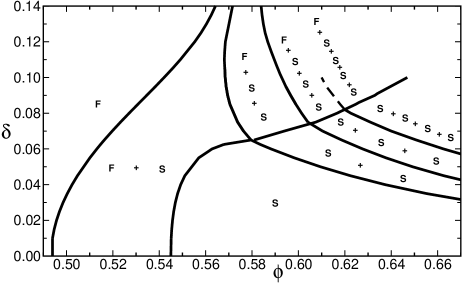
Figure 9: Full phase diagram for polydisperse hard spheres with a triangular size distribution. In each region the nature of the phase(s) coexisting at equilibrium is indicated (F: fluid, S: solid). Dashed line: best guess for the phase boundary in the region where our numerical data become unreliable. From FasSol03 .

Fig. 9 shows the full phase diagram for the triangular parent distribution. In each region the nature of the phase(s) coexisting at equilibrium is indicated. The cloud curves of Fig. 4 (a) reappear as the boundaries between single-phase regions and areas of phase coexistence. Starting from the onset of solid-solid separation and increasing density or $\delta$, fractionation into multiple solids occurs. The overall shape of the phase boundaries in this region is in good qualitative agreement with the approximate calculations of Bartlett98 , see Fig. 3, though as discussed below the details of the fractionation behaviour are rather different. We find up to 4 coexisting solids. At larger $\delta$ than we can tackle numerically, phase splits into 5 or more solids would be expected since each individual solid can only tolerate a finite amount of polydispersity. However, from Fig. 9 such phase splits would occur at increasing densities and eventually be limited by the physical maximum volume fraction $\phi_{c}\approx 74\%$. Also, at higher $\delta$ more complicated single-phase crystal structures, with different lattice sites occupied preferentially by (say) smaller and larger spheres, could appear and compete with the substitutionally disordered solids we consider.

A feature of the phase diagram in Fig. 9 not predicted in previous work is the coexistence of a fluid with multiple solids. However, that a three-phase F-S-S region must occur was already indicated by the triple point which we found earlier on the solid cloud curves. As in the case of solid-solid phase splits, coexistences involving more than two solids – and a fluid – then appear with increasing $\delta$.

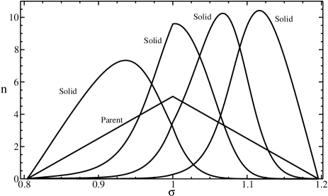
Figure 10: Normalised size distribution of four coexisting solid phases obtained from a parent distribution with $(\phi,\delta)=(0.63,0.08)$. From left to right, the solids have volume fractions and polydispersities $(0.601,0.054)$, $(0.629,0.046)$, $(0.646,0.040)$, $(0.663,0.036)$. From FasSol03 .

We consider the fractionation behaviour in the multiphase regions more systematically in the next section. Before doing so, a few qualitative statements are in order. In Fig. 10 we show a sample plot of the normalised diameter distributions $n(\sigma)=\rho(\sigma)/\rho_{0}$ of four coexisting solids. This shows that fractionated solids do not, as one might naively assume Bartlett98 , split the diameter range of the parent evenly among themselves. The polydispersities of the coexisting phases are in fact rather different; in Fig. 10 they range from $\delta=0.036$ to $0.054$ for a parent with $\delta=0.08$. There is in fact a strong correlation between the polydispersity of a fractionated solid and its volume fraction: solids with lower volume fraction $\phi$ tend to have higher polydispersity $\delta$. This conclusion is intuitively appealing since higher compression should disfavour a polydisperse crystalline packing.

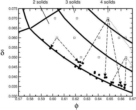
Figure 11: The properties of the daughter solids (circles) arising by phase separation from some chosen parents (squares) across the phase diagram. Plotted are polydispersity $\delta$ versus volume fraction $\phi$. The arrows show the daughter phases for three parents explicitly; as indicated by the dotted lines, not all daughter phases are within the range of the plot. Note the clustering of all daughter phases near the solid cloud curve.

We have studied the relation between polydispersity and volume fraction more quantitatively, by plotting $\delta$ vs $\phi$ for all the “daughter” solids that arise by phase separation from a number of different parents across the phase diagram. We find a set of points (Fig. 11) that cluster very closely around the high-density branch of the solid cloud curve, emphasising the tight correlation between $\delta$ and $\phi$. Note that some of the points fall above the solid cloud curve. This is not a contradiction because the latter marks the onset of instability against phase separation only for solids with a triangular size distribution, whereas the daughter phases plotted here can have rather different size distributions (compare Fig. 10).

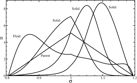
Figure 12: Normalised diameter distributions for F-S-S-S phase coexistence obtained from a parent distribution with $(\phi,\delta)=(0.603,0.08)$. From FasSol03 .

As part of our qualitative overview of fractionation behaviour, we show next in Fig. 12 the size distributions for a situation where a fluid coexists with three solids. The general trend which we observed from the cloud and shadow curves, namely for the solid(s) to contain the larger particles, is found confirmed here. However, the details of the fractionation are again nontrivial: while the coexisting fluid is enriched in the smaller particles as expected, it also contains “left over” large spheres that did not fit comfortably into the solid phases. It thus in fact ends up having a larger polydispersity (0.104) than the parent (0.08) in this example.

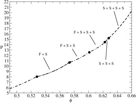
Figure 13: The osmotic pressure plotted as a function of the parent volume fraction along a dilution line, for a triangular parent with polydispersity $\delta=0.08$. Phase boundaries are marked by full circles; line segments are annotated with the nature of the phases (fluid/solid) in the different coexistence regions.

Finally, an indirect manifestation of fractionation is provided by the variation of the osmotic pressure along a dilution line. In a monodisperse system, the pressure remains constant throughout any phase coexistence region because the properties of the coexisting phases do not change; only the fractions of system volume vary which these phases occupy. In a polydisperse system, on the other hand, the composition of the coexisting phases varies as the coexistence region is traversed. We illustrate this in Fig. 13 for a triangular parent size distribution with $\delta=0.08$. It is striking that the variation of the pressure with volume fraction is almost smooth, even though a number of phase boundaries are crossed.

V Fractionation behaviour

We proceed in this section to a systematic study of the fractionation behaviour of polydisperse hard spheres, having discussed its qualitative features above. To this end we extend the classical visual representations in terms of cloud and shadow curves and overall phase diagrams to include more detailed information about the properties of the coexisting daughter phases. To obtain insights into the effects of varying both the parent’s volume fraction and its polydispersity, 3-D plots will be particularly useful here. In a second part we ask whether there is an optimal way of making the separation between fractionated phases visible, and suggest principal component analysis (PCA) as a method for achieving this. We focus throughout on the range of parent polydispersities $0.04<\delta<0.08$, which covers all the various coexistence regions in the phase diagram of Fig. 9. Where it is necessary to distinguish the volume fraction and polydispersity of the parent from those of the daughter phases, we will add the superscript $(0)$, writing $\phi^{(0)}$ and $\delta^{(0)}$.

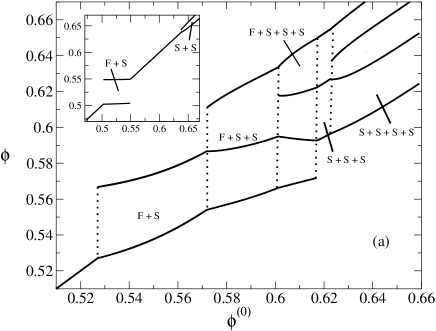
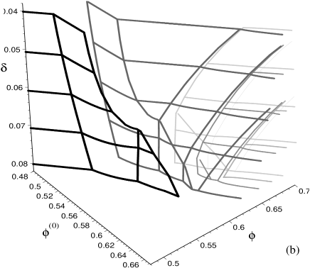
Figure 14: (a) Volume fraction $\phi$ of the various coexisting daughter phases versus the volume fraction $\phi^{(0)}$ of the parent phase, for $\delta=0.08$ (main graph) and $\delta=0.04$ (inset). (b) 3-D plot showing the dependence of the $\phi$ on $\phi^{(0)}$ and the parent’s polydispersity $\delta$. Different phases are represented by different grey levels. Note that the $\delta$-axis is plotted upside down for better visibility. The top and bottom slices correspond to the 2-D plots in (a).

We start with a 2-D plot showing the volume fraction of the coexisting phases versus the volume fraction of the parent phase, Fig. 14 (a), for two parent polydispersities $\delta$. For a narrow parent size distribution ($\delta=0.04$, inset), we see that the behaviour in the F-S coexistence region is similar to what would be expected for a monodisperse system, with the volume fractions of the daughter phases remaining essentially constant. Only at large $\phi^{(0)}$ does the polydisperse nature of the system become fully apparent, through the occurrence of S-S phase separation. For a parent with $\delta=0.08$, on the other hand, the properties of the daughter phases vary strongly with $\phi^{(0)}$. In the S+S+S and S+S+S+S regions in particular, the volume fractions of the daughter solids increase systematically with $\phi^{(0)}$: fractionation from a denser parent here produces denser daughter phases, rather than varying proportions of daughters with fixed densities.

To demonstrate more explicitly the change in behaviour as the parent polydispersity $\delta$ increases, we show in Fig. 14 (b) a 3-D plot of the daughter volume fractions $\phi$ versus $\phi^{(0)}$ and $\delta$. The orientation of the axes has been chosen such that horizontal cuts through the plot represent fixed $\delta$, with the top and bottom planes corresponding to the data shown in the 2-D plots of Fig. 14 (a). A benefit of the 3-D representation is that each daughter phase now corresponds simply to a separate surface. Each surface ends at the phase boundary where the relevant phase disappears from the phase split. The disappearance or appearance of any phase then causes kinks in the other surfaces. As expected, only the fluid surface extends to the lowest $\phi^{(0)}$. As $\phi^{(0)}$ is increased, the “conventional” solid which also exists in the monodisperse limit makes its first appearance. A further three fractionated solids then eventually appear one after the other. These are polydispersity-induced, i.e. have no analogue in the monodisperse system, and the surfaces representing them do not extend to $\delta\to 0$.

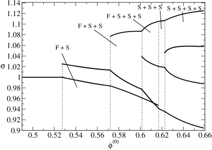
Figure 15: Mean diameter of coexisting phases plotted against parent volume fraction $\phi^{(0)}$, for parent polydispersity $\delta=0.08$. The dashed lines delineate the various phase coexistence regions.

Having clarified the variation of the volume fractions of the daughter phases across the phase diagram, we show their mean diameters in Fig. 15, plotted against parent volume fraction at fixed (parent) polydispersity $\delta=0.08$. One observes clearly the general trend for the solid phases to contain larger particles than the fluid. An exception to this occurs in the F+S+S+S coexistence region, where the fluid has a slightly larger mean diameter than one of the solids. The explanation for this can be found in our earlier discussion of Fig. 12: in addition to the smallest spheres, the fluid can also contain some of the larger spheres that are not accommodated in any of the solids, and this pushes up its mean diameter. The second qualitative trend demonstrated by Fig. 15 is that the coexisting solids tend to split the range of particle diameters in the parent distribution amongst themselves, with almost equidistant mean diameters. As the parent volume fraction increases, the strength of this fractionation effect is seen to grow, and the mean diameters become increasingly separated from each other.

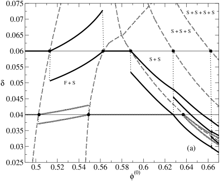
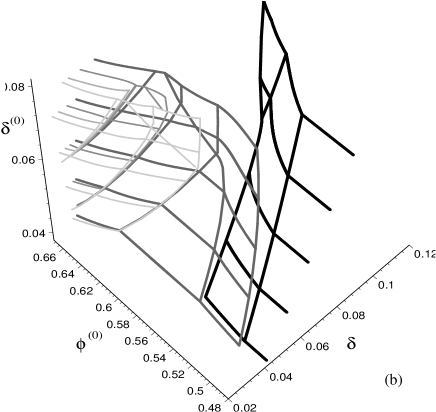
Figure 16: (a) Plot of the polydispersities of coexisting phases along two dilution lines (thin horizontal lines), i.e. as a function of the parent volume fraction for fixed parent polydispersity $\delta^{(0)}=0.04$ and $0.06$. The dashed lines indicate the phase boundaries in the $(\phi^{(0)},\delta^{(0)})$-plane; phases appear or disappear at the points where the horizontal line corresponding to the fixed parent polydispersity intersects these phase boundaries (full circles). (b) Corresponding 3-D plot, showing the daughter polydispersities $\delta$ against the parent volume fraction $\phi^{(0)}$ and parent polydispersity $\delta^{(0)}$.

Finally, we examine the relationship between the polydispersities $\delta$ of the different daughter phases and the volume fraction $\phi^{(0)}$ and polydispersity $\delta^{(0)}$ of the parent. Fig. 16 (a) shows 2-D plots of the daughter polydispersities versus $\phi^{(0)}$, at $\delta^{(0)}=0.04$ and $0.06$. As expected, for the more polydisperse parent there are significant variations of the daughter polydispersities across the coexistence regions. Where multiple solids coexist, their polydispersities decrease with increasing parent volume fraction. This is consistent with the general trend that denser solids tend to be less polydisperse. In the 3-D plot of Fig. 16 (right), this same trend also causes the surfaces corresponding to the various solids to have rather similar shapes in the region of solid-solid coexistence. For the fluid, on the other hand, the graph demonstrates that it always has a larger polydispersity than the parent, arising from the presence of large particles “left over” from the solid phases (see Fig. 12).

V.1 Principal components analysis

The above plots of aspects of fractionation behaviour lead naturally to the question of whether there is a “maximally fractionating” property, i.e. one which most strongly reveals the differences between the various coexisting phases across the phase diagram. We focus on properties which are generalised moments of the density distribution, of the form $r=\int\!d\sigma\,f(\sigma)\rho(\sigma)$ with some weight function $f(\sigma)$. While not all properties can be expressed in this way – the polydispersity $\delta$, for example, involves squares and ratios of such moments – this is still a fairly large class of measurable properties; e.g. setting $f(\sigma)=1$ would give us the number density, $f(\sigma)=\sigma^{3}$ the volume fraction, $f(\sigma)=\sigma$ the mean diameter times the number density etc.

Suppose now that we have a number of measurements of $\rho(\sigma)$, specifically the daughter density distributions that arise within some region of the phase diagram. We can think of the $\rho(\sigma)$ as points in a high-dimensional (in fact infinite-dimensional) space, and of our desired moment $r$ as a projection along the direction defined by $f(\sigma)$ SolWarCat01 . A good choice for a maximally fractionating property would then be to maximise the variance of our moment among the various measured $\rho(\sigma)$. This can be done by Principal Component Analysis (PCA), a method designed to select directions of large variance Bishop95 . Mathematically, the requirement of maximum variance can be written as

$${\rm max}_{f(\sigma)}\int\!d\sigma\,d\sigma^{\prime}\,f(\sigma)A(\sigma,\sigma^{\prime})f(\sigma^{\prime})$$ (18)

subject to $\int\!d\sigma\,f^{2}(\sigma)=1;$ here $A(\sigma,\sigma^{\prime})$ is the (infinite-dimensional) covariance matrix of our measurements. We define this as $A(\sigma,\sigma^{\prime})=\langle[\rho(\sigma)-\rho^{(0)}(\sigma)][\rho(\sigma^{\prime})-\rho^{(0)}(\sigma^{\prime})]\rangle$. The average here is over all our measurements of $\rho(\sigma)$, and we subtract off for each $\rho(\sigma)$ the corresponding parent distribution $\rho^{(0)}(\sigma)$. This effectively removes the average of the various measured $\rho(\sigma)$ because, from particle conservation (8), the parent is a weighted average over the various daughter phases. An alternative definition of $A$ would be to remove the actual measurement average, $A(\sigma,\sigma^{\prime})=\langle[\rho(\sigma)-\langle\rho(\sigma)\rangle][\rho(\sigma^{\prime})-\langle\rho(\sigma^{\prime})\rangle]\rangle$. In our numerical experiments described below, this lead to almost indistinguishable results.

The maximisation problem (18) is in principle over an infinite-dimensional function space. To arrive at a more practical task, we restrict the search to a subspace by requiring the weight function to be of the form $f(\sigma)=\sum_{i=0}^{3}\alpha_{i}\sigma^{i}$. This corresponds to searching for a maximally fractionating property among those expressible as linear combinations of the moments $\rho_{0},\ldots,\rho_{3}$, i.e. $r=\sum_{i=0}^{3}\alpha_{i}\rho_{i}$ With this simplification, the problem (18) reduces to

$${\rm max}_{\alpha}\ \alpha^{T}C\alpha\quad\mbox{subject to}\quad\alpha^{T}D\alpha=1$$ (19)

Here $\alpha$ denotes the vector with elements $\alpha_{0},\ldots,\alpha_{3}$ and the $4\times 4$ matrix $C$ is defined as

$$C_{ij}=\int\!d\sigma\,d\sigma^{\prime}\,\sigma^{i}A(\sigma,\sigma^{\prime})(\sigma^{\prime})^{j}=\langle(\rho_{i}-\rho^{(0)}_{i})(\rho_{j}-\rho^{(0)}_{j})\rangle$$

which is just the covariance matrix of the moments, with the parent moments again subtracted off. The matrix $D$, on the other hand, is given by $D_{ij}=\int\!d\sigma\,\sigma^{i+j}$. The $\sigma$-integration range has to be bounded to make this well-defined. In our case of a triangular parent distribution the obvious choice, adopted here, is to make this range equal to the range of particle sizes occurring in the parent.

Imposing the constraint in (19) via a Lagrange multiplier shows that solution vectors $\alpha$ must obey $C\alpha=\lambda D\alpha$, or equivalently $D^{-1/2}CD^{-1/2}(D^{1/2}\alpha)=\lambda D^{1/2}\alpha$. The solutions can thus be obtained by an eigenvalue decomposition of the matrix $D^{-1/2}CD^{-1/2}$, with $\lambda$ the eigenvalue and $D^{1/2}\alpha$ the corresponding eigenvector. (Numerically, it is more convenient to solve the equivalent problem of finding the eigenvalues and right eigenvectors of the matrix $D^{-1}C$.) The eigenvectors are termed principal components, and the $\lambda$’s give the variance captured by each principal component. The most important principal component, and the one of interest to us, is then the one with the largest $\lambda$.

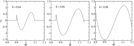
Figure 17: Principal component weight function, $f(\sigma)$, obtained from data along dilution lines for three different values of parent polydispersity 0.04, 0.06 and 0.08. The range of $\sigma$-values where $f(\sigma)\neq 0$ is in each case that over which the parent density distribution is nonzero, i.e. the range of particle sizes actually occurring in the system.

We have implemented this PCA search for maximally fractionating properties by considering as our measured $\rho(\sigma)$ the daughter phases as they occur along a dilution line. We do this separately for triangular parent distributions of polydispersity 0.04, 0.06 and 0.08, respectively, because different ranges of particle size $\sigma$ are relevant in the three cases. The resulting weight functions $f(\sigma)$ are plotted in Fig. 17. One sees that in all cases, $f(\sigma)$ is to a good approximation a combination of the odd weight functions $\sigma$ and $\sigma^{3}$, with the coefficients such that $f(\sigma)$ crosses zero near the edge of the $\sigma$-range. Loosely speaking, the function $f(\sigma)$ can be interpreted as an approximation to ${\rm sgn}(\sigma-1)$ within the space spanned by $\sigma^{0},\ldots,\sigma^{3}$, i.e. by a third-order polynomial in $\sigma$. It thus effectively measures the difference in number density between particles above and below the mean parental diameter. This is an intuitively appealing measure of fractionation behaviour.

Finally, Fig. 18 shows the properties of the daughter phases as measured by the maximally fractionating observable selected by PCA. The overall features of the plot on the right, for parent polydispersity $\delta=0.08$, are not dissimilar to the mean diameter representation in Fig. 15, so that the benefit of PCA in this problem is relatively modest. Some interesting features are accentuated by PCA, however; e.g. the crossover between the fluid and solid lines is more pronounced in Fig. 18, demonstrating clearly how the fluid size distribution acquires a significant fraction of the larger particles. We expect that the benefits the PCA method of selecting maximally fractionating properties should become more pronounced in systems with several polydisperse attributes $\sigma$, e.g. particle size and charge. Suitable properties for revealing fractionation behaviour could then depend on combinations of these attributes, which can be systematically found using PCA.

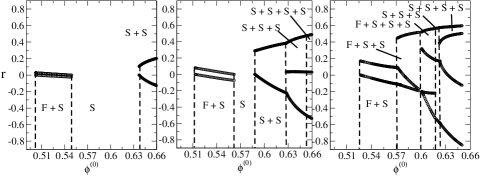
Figure 18: Maximally fractionating moment (as selected by PCA) for coexisting daughter phases, plotted against parent volume fraction $\phi^{(0)}$ at parent polydispersity $\delta=0.04$, 0.06 and 0.08 (from left to right).

VI Comparison with perturbative theories and Monte Carlo simulations

In this section we validate our theoretical predictions in two ways. First, we compare to perturbative theories for near-monodisperse parents, which predict qualitatively how the properties of coexisting phases should vary as the parent is made increasingly polydisperse. Second, we compare quantitatively to Monte Carlo simulations of polydisperse hard spheres with an imposed chemical potential distribution.

VI.1 Near-monodisperse systems

For systems that are nearly monodisperse, one can make general statements about the fractionation behaviour by considering deviations of particle diameters from the mean as small and performing a perturbation expansion EvaFaiPoo98 ; Evans01 . This approach presupposes, of course, that the phase separation of interest occurs already in the monodisperse reference system. In our hard sphere case it is therefore applicable only to fluid-solid coexistence. Phase separation involving several solid phases is induced by polydispersity itself and cannot be treated perturbatively.

A strong prediction of the perturbative approach is that the difference in mean particle diameters of two coexisting phases, $\Delta\bar{\sigma}=\bar{\sigma}^{(1)}-\bar{\sigma}^{(2)}$ is universally related to the parental polydispersity $\delta$ via

$$\Delta\bar{\sigma}\propto\delta^{2}.$$ (20)

An increase in the width of the parent size distribution thus contributes only at second order to the mean diameter difference. The proportionality coefficient in this relation is non-universal and depends on the properties of the phase separation in the corresponding monodisperse reference system. Equation (20) is the leading term in a perturbation expansion in $\delta$ at fixed density of the parent. The volume fraction $\phi$ then varies with $\delta$; for symmetric size distributions it increases. If instead $\phi$ is held constant as $\delta$ is varied, the perturbation expansion is modified, though the leading term (20) remains unaffected.

A relation analogous to equation (20) applies to the difference in polydispersities $\Delta\delta=\delta^{(1)}-\delta^{(2)}$ of the daughter phases. For symmetric parent size distributions, one finds

$$\Delta{\delta}\propto\delta^{3}\;.$$ (21)

so that an increase in the parent polydispersity $\delta$ only affects $\Delta\delta$ at third order.

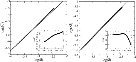
Figure 19: Log-log plots of the difference in mean diameters (left) and in polydispersity (right) for coexisting fluid-solid phases at parent density $\rho=0.52$, plotted against parent polydispersity $\delta$. The solid lines show the theoretically expected power laws, Eqs. (20) and (21), with the proportionality constants fitted by eye to the numerical data. The insets show the ratios $\Delta\bar{\sigma}/\delta^{2}$, $\Delta{\delta}/\delta^{3}$, which from the theory are expected to approach constants for $\delta\to 0$. The data are consistent with this (note the narrow ranges displayed on the $y$-axes).

To verify the above perturbative predictions, we determined the mean diameters and polydispersities of the daughter phases for fluid-solid separation at parent density $\rho=0.52$ and parent polydispersity $\delta$ ranging from $0.02$ to $0.086$. Fig. 19 shows log-log plots of $\Delta\bar{\sigma}$ and $\Delta\delta$ against $\delta$, confirming the predicted power laws. The insets show the ratios $\Delta\bar{\sigma}/\delta^{2}$ and $\Delta\delta/\delta^{3}$. Our data are again consistent with the theoretical expectation that these ratios should approach constants in the limit of small $\delta$. Overall, the scaling predictions of perturbative theories for near-monodisperse systems are fully obeyed by our data.

Finally, to emphasise the point that perturbative approaches do not apply to phase separations that are caused by polydispersity, we show in Fig. 20 the evolution of the polydispersity of coexisting solids as the parent polydispersity is increased, at fixed parent density $\rho=0.62$. As the inset shows, there is now no simple relationship akin to (21) which relates the difference in the polydispersities of the daughter solids to the $\delta$ of the parent. In fact, the perturbative limit of small $\delta$ is not even defined here, since the solid-solid phase separation only occurs above a nonzero (density-dependent) threshold value of $\delta$.

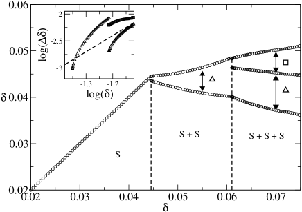
Figure 20: Plot of the polydispersity of coexisting solids versus the polydispersity $\delta$ of the parent phase. The parent number density is kept constant at $\rho=0.62$ while the latter is varied. The inset shows the log-log plot of the difference of the polydispersities $\Delta\delta$ in the S+S and S+S+S region versus $\delta$ and the slope of the theoretically expected power law (21) (dashed line). This demonstrates that the perturbative prediction for the scaling of $\Delta\delta$ with $\delta$ does not apply here.

VI.2 Comparison with Monte Carlo simulations

As discussed in the preceding sections, our theoretical results for fluid-solid coexistence in polydisperse hard sphere systems are in qualitative agreement with numerical simulations BolKof96 ; BolKof96b ; KofBol99 , in particular concerning the coexistence of rather polydisperse fluids with solids that have a much narrower size distributions. There is, however, an important difference: our calculations apply to the experimentally realistic case where an overall parent density distribution is fixed. The simulations, on the other hand, are performed at imposed chemical potential differences, with the actual size distributions in the coexisting phases varying strongly across the phase diagram. In order to obtain a quantitative comparison between theory and simulations, we calculate explicitly in this section the theoretical predictions for the – somewhat unrealistic – scenario addressed in the simulations. We will find good quantitative agreement, thus validating our approach and, in particular, our choice of free energy expressions for the fluid and solid phases.

The simulations of BolKof96 ; BolKof96b ; KofBol99 were carried out in an isobaric semi-grandcanonical ensemble, which corresponds to fixed particle number $N$, pressure $P$ and chemical potential differences $\mu(\sigma)-\mu(\sigma_{b})$. Here $\sigma_{b}$ is the diameter of a reference particle. The advantage of the semi-grandcanonical ensemble is that it allows many different realizations of the particle size distribution to be sampled, thus minimising finite-size effects. The fixed particle number $N$, on the other hand, avoids simulation moves where particles need to be inserted into dense fluids or solids.

Bolhuis and Kofke BolKof96 ; BolKof96b considered specifically a quadratic form for the chemical potential differences,

$$\mu(\sigma)-\mu(\sigma_{b})=-\frac{(\sigma-\sigma_{b})^{2}}{2\nu}.$$ (22)

The activity $\exp[\mu(\sigma)]$ thus has a Gaussian shape of variance $\nu$. For small $\nu$, one expects the activity distribution to set the size distributions in the coexisting phases, which should therefore have polydispersity $\delta=\nu^{1/2}$; $\nu\to 0$ recovers the monodisperse case. The reference diameter $\sigma_{b}=1$ is held fixed as $\nu$ is increased from zero. The pressure $P$ is then adapted by Gibbs-Duhem integration Kofke93 to follow the line of fluid-solid phase coexistence in the $(\nu,P)$-plane.

In order to reproduce the situation considered in the simulations using our theoretical approach, we will study a system with prior $R(\sigma)=\exp[-(\sigma-1)^{2}/(2\nu)]$. The moment free energy then gives the free energy of phases with density distributions of the form (cf. (12))

$$\rho(\sigma)=\exp\left[-\frac{(\sigma-1)^{2}}{2\nu}+\sum_{i=0}^{3}\lambda_{i}\sigma^{i}\right]$$

From (6), the corresponding chemical potentials have the form

$$\mu(\sigma)=\ln\rho(\sigma)+\sum_{i=0}^{3}\mu^{\rm ex}_{i}\sigma^{i}=-\frac{(\sigma-1)^{2}}{2\nu}+\sum_{i=0}^{3}(\lambda_{i}+\mu^{\rm ex}_{i})\sigma^{i}$$ (23)

Now the $\lambda_{i}+\mu^{\rm ex}_{i}$ are just the moment chemical potentials $\mu_{i}=\partial f_{\rm mom}/\partial\rho_{i}$. So if we apply the moment free energy but treat the moment densities $\rho_{1}$, $\rho_{2}$, $\rho_{3}$ as non-conserved, the associated $\mu_{i}$ are forced to vanish automatically at equilibrium. The sum over $i$ in (23) then reduces to a constant, $\mu_{0}=\lambda_{0}+\mu^{\rm ex}_{0}$, and we have precisely the chemical potential differences (22) used in the simulations. In summary, applying the MFE method with a Gaussian prior and $\rho_{0}$ the only conserved moment, we increase $\rho_{0}$ from zero until coexistence with a solid phase is first found. This is then the desired fluid-solid coexistence for quadratic chemical potential differences, and we can determine in particular the pressure $P$ at coexistence. Repeating this process for a range of values of $\nu$ gives the coexistence curve in the $(\nu,P)$-plane.

Our actual implementation of this approach has one minor difference. In the simulations it is observed that the mean diameters in the coexisting phases decrease significantly as $\nu$ is increased, eventually becoming much smaller than $\sigma_{b}$. For our numerical work, however, it is desirable to keep the size distributions within a fixed range, e.g. in order to ensure that our chemical potentials for the solid phase remain reliable. To achieve this, we treat not just $\rho_{0}$ but also $\rho_{1}$ as conserved. Keeping $\rho_{1}/\rho_{0}=1$ as $\rho_{0}$ is varied then ensures that the fluid phase always has unit mean diameter, and the particle sizes in the coexisting solid are expected to be comparable. This ensures that we can use a fixed $\sigma$-range for all calculations, for which we choose $\sigma\in[0.7,1.3]$.

With $\rho_{0}$ and $\rho_{1}$ both conserved, the chemical potentials (23) become

$$\mu(\sigma) = -\frac{(\sigma-1)^{2}}{2\nu}+\mu_{0}+\mu_{1}\sigma$$ (24)

$$= -\frac{(\sigma-1-\nu\mu_{1})^{2}}{2\nu}+\frac{1}{2}\nu\mu_{1}^{2}+\mu_{1}+\mu_{0}$$ (25)

which is again of the form (22) but now with a varying reference diameter $\sigma_{b}=1+\nu\mu_{1}$. The corresponding scaled quantities that are to be compared to $\nu$ and $P$ from the simulations are then $\nu/\sigma_{b}^{2}$ and $P\sigma_{b}^{3}$ . Note finally that our numerical implementation again uses centred moments, with weight functions $[(\sigma-1)/\delta_{0}]^{i}$ rather than $\sigma^{i}$, but this causes no conceptual differences. In particular, keeping the standard moments $\rho_{0}$ and $\rho_{1}$ conserved is equivalent to conservation of the centred moments with $i=0$ and $i=1$, because of the linear relations between the two sets of moments.

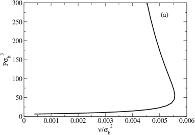
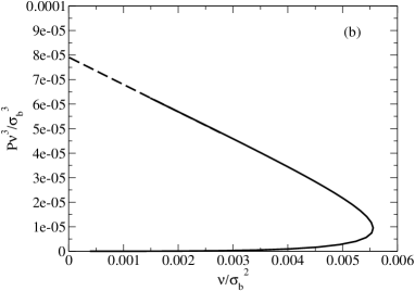
Figure 21: (a) Solid-fluid coexistence pressure $P\sigma_{b}^{3}$ as a function of the imposed width $\nu/\sigma_{b}^{2}$ of the activity distribution. Both are scaled appropriately with $\sigma_{b}$ to account for the fact that $\sigma_{b}$ varies in our calculation but is held constant in the simulations. (b) The pressure is rescaled to $P\sigma_{b}^{3}(\nu/\sigma_{b}^{2})^{3}=P\nu^{3}/\sigma_{b}^{3}$ to show the limiting behaviour for $\nu/\sigma_{b}^{2}\to 0$.

Fig. 21 (a) shows our results for the coexistence curve in the $(\nu/\sigma_{b}^{2},P\sigma_{b}^{3})$-plane. As $\nu$ increases (starting from the bottom left corner), both $P\sigma_{b}^{2}$ and $\nu/\sigma_{b}^{2}$ initially increase. However, eventually $\nu/\sigma_{b}^{2}$ reaches a maximum value $\nu_{\rm max}=\nu/\sigma_{b}^{2}=0.0056$. At this point, the slope $d(P\sigma_{b}^{3})/d(\nu/\sigma_{b}^{2})$ becomes infinite. On further increasing $\nu$, the coexistence curve then bends back, with $\nu/\sigma_{b}^{2}$ decreasing towards zero while the pressure diverges. Bolhuis and Kofke BolKof96 argued that this divergence arises because the pressure is measured on the scale of the mean $\sigma_{b}$ of the activity distribution, while the typical particle diameters in the coexisting phases become much smaller than $\sigma_{b}$, by a factor scaling as $\nu/\sigma_{b}^{2}$. The rescaled pressure $P\sigma_{b}^{3}(\nu/\sigma_{b}^{2})^{3}=P\nu^{3}/\sigma_{b}^{3}$ should therefore approach a constant value in the limit $\nu/\sigma_{b}^{2}\to 0$. The simulations were consistent with this expectation, and our theoretical results in Fig. 21 (b) are in full agreement. By extrapolation, we estimate the limiting or ‘terminal’ value of the rescaled pressure, i.e. the point where the rescaled coexistence curve intersects the vertical axis, as $P_{\rm t}=7.9\times 10^{-5}$.

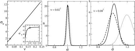
Figure 22: Left: Plot of $\sigma_{b}$ as a function on $\nu$. The inset shows the derivative $d\sigma_{b}/d\nu$. As expected, $\sigma_{b}$ grows linearly as $\nu$ becomes large. The star indicates the value of $\nu$ at which $\nu/\sigma_{b}^{2}$ reaches its maximum and the slope of the pressure plots in Fig. 21 becomes infinite. Middle and right: Normalised size distributions $n(\sigma)$ of the coexisting fluid (dashed line) and solid (solid line) phases. The dotted curve gives the shape of the activity distribution $\exp(\mu(\sigma))$. Middle: For $\nu=0.02^{2}$, fluid and solid have essentially identical size distributions of polydispersity $\delta\approx\nu^{1/2}=0.02$; the corresponding value of $\sigma_{b}$ is 1.02. Right: For $\nu=0.08^{2}$, the size distributions are significantly different from each other and from the activity distribution, which is now centred around $\sigma_{b}=1.19$.

The scaling mentioned above implies that, as $\nu$ becomes large, the mean particle diameter in the coexisting phases will be of order $\sigma_{b}(\nu/\sigma_{b}^{2})=\nu/\sigma_{b}$, rather than $\sigma_{b}$. In our scheme, where the mean diameter in the fluid is fixed at unity, $\sigma_{b}$ should thus become linear in $\nu$. As shown in Fig. 22 (left), this is indeed what we find. A plot of the numerical derivative of this dependence, in the inset of Fig. 22 (left), also reveals that at small $\nu$-values – below those where $\nu/\sigma_{b}^{2}$ reaches its maximum – the behaviour is no longer exactly linear. This is to be expected considering that $\sigma_{b}=1+\nu\mu_{1}$ depends on both $\nu$ and $\mu_{1}$.

The plots in the middle and on the right of Fig. 22 show particle size distributions in the coexisting fluid and solid phases at two different values of $\nu$. For small $\nu=0.02^{2}$, the distributions are essentially identical and have width $\delta\approx\nu^{1/2}=0.02$ as expected; they are also close to the activity distribution, which has its peak at $\sigma_{b}=1.02$ for this $\nu$. For larger $\nu=0.08^{2}$, on the other hand, there is significant fractionation between the fluid and the solid. One can now also clearly see how the mean particle diameters – which are exactly unity in the fluid, by construction, and around 1.02 in the solid – become smaller than the mean of the activity distribution, which is $\sigma_{b}=1.19$ for this value of $\nu$.

To summarise the properties of the coexisting fluid and solid phases, we plot them in a volume fraction–polydispersity phase diagram, shown in Fig. 23.

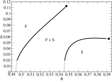
Figure 23: Phase diagram for fluid-solid coexistence with imposed quadratic chemical potential differences. Plotted is the polydispersity $\delta$ versus the volume fraction $\phi$ of the coexisting fluid and solid phases; $\nu$ increases from bottom left to top right along the curves. The circles indicate the terminal points reached by extrapolating to $\nu\to\infty$. The dotted lines sketch the approach to the known monodisperse limit $\nu\to 0$.

As discussed in detail in BolKof96 , a feature which is at first surprising is that the curves terminate, with the properties of the coexisting phases approaching finite limits for $\nu\to\infty$. One has to bear in mind, however, that the occurrence of such terminal points is directly linked to the shape of the imposed chemical potential distribution and so not physically very meaningful. Indeed, other shapes can and do give fluids and solids with larger $\phi$ and/or $\delta$ KofBol99 .

We obtain the location of the terminal points by plotting our numerical predictions against $1/\nu$ and extrapolating to $1/\nu=0$.

Quantity	Bolhuis and Kofke BolKof96	Present work
$\nu_{\rm max}$	0.0056	0.0056
$P_{\rm t}$	7.9 $\times 10^{-5}$	7.9 $\times 10^{-5}$
$(\phi_{\rm t,f},\delta_{\rm t,f})$	(0.545, 0.12)	(0.548, 0.113)
$(\phi_{\rm t,s},\delta_{\rm t,s})$	(0.575, 0.057)	(0.592, 0.057)

Table 2: Comparison between some characteristic quantities of fluid-solid coexistence at imposed chemical potential distribution, as determined in simulations BolKof96 and in the present theoretical study. Here $\nu_{\rm max}$ is the maximum value of $\nu/\sigma_{b}^{2}$, $P_{\rm t}$ the terminal value of the rescaled pressure $P\nu^{3}/\sigma^{3}_{b}$ in the limit $\nu/\sigma_{b}^{2}\to 0$, $\phi_{\rm t,f/s}$ the terminal volume fraction for the fluid/solid phases and $\delta_{\rm t,f/s}$ the corresponding terminal polydispersity.

The resulting values are compared in Table 2 with those obtained in the simulations of BolKof96 . We find excellent quantitative agreement for $\nu_{\rm max}$, defined as the maximum value of $\nu/\sigma_{b}^{2}$, and $P_{\rm t}$, the terminal value of the rescaled pressure $P\nu^{3}/\sigma^{3}_{b}$. Similar comments apply to the volume fractions and polydispersities at the terminal points of the fluid and solid coexistence curves in Fig. 23. Only the terminal volume fraction of the solid is over-estimated somewhat, but even here the deviation is less than $3\%$.

In conclusion, our theoretical predictions for fluid-solid coexistence at imposed chemical potential differences are not just in qualitative but in fact quantitative agreement with the outcomes of Monte Carlo simulations. This provides strong validation for our approach. It demonstrates in particular that our chosen model free energies for the hard sphere fluid and solid are accurate, at least in the range of relatively small polydispersities studied here.

VII Conclusion and outlook

We have studied the equilibrium behaviour of size-polydisperse hard spheres, starting from accurate free energy expressions for the hard sphere solid and fluid. Cloud and shadow curves, which locate the onset of phase coexistence, were found exactly by using the moment free energy (MFE) method. We were also able to calculate the full phase diagram, however, by using the MFE results as starting points for a solution of the full phase equilibrium equations.

In contrast to earlier simplified theoretical treatments, we found no point of equal concentration between fluid and solid. Rather, the fluid cloud curve continues to larger polydispersities while the coexisting solid shadow always has a polydispersity $\delta$ below a “terminal” value of around $\delta_{\rm t}\approx 0.06$. In this sense the concept of terminal polydispersity only applies to the solid phase, while any experimentally observed terminal polydispersity from the fluid side must be attributed to non-equilibrium effects such as an intervening kinetic glass transition PusVan87 , large nucleation barriers AueFre01 or the unusual growth kinetics of polydisperse crystals EvaHol01 .

Concomitant with the absence of the point of equal concentration, we also found no re-entrant melting. Instead, a sufficiently compressed polydisperse solid fractionates into two or more solid phases; our results in this region of the phase diagram are consistent with previous approximate calculations. In addition, we found that coexistence of several solids with a fluid phase is also possible. That such phase splits must exist is clear from the fact that the solid cloud curve has two branches, describing onset of fluid-solid and solid-solid phase separation at low and high densities respectively; a fluid-solid-solid coexistence region begins where these meet.

We then analysed the fractionation behaviour in detail. As a general rule, the fluid phases contain the smaller particles in the system, while the larger ones are found predominantly in the solid phases. The solid phases have smaller polydispersities $\delta$ than the parent phase; this is as expected since narrower particle size distributions are more easily accommodated on a regular lattice. Consistent with this physical intuition, we also found that there is a strong correlation between the polydispersity $\delta$ and the volume fraction $\phi$ of coexisting solids, with the denser phases (larger $\phi$) having smaller $\delta$. For the fluid phases, on the other hand, we found larger polydispersities than in the parent. This is because the fluid contains, together with a relatively narrow distribution of smaller particles, also residual larger particles that were not incorporated into any of the solid phases.

Three-dimensional fractionation plots transparently showed the continuity of the properties of the various phases across the phase diagram, with each corresponding to a distinct surface. The individual phases change significantly as coexistence regions are traversed; this is in contrast to monodisperse systems, where only the amounts of coexisting phases vary. Correspondingly, the pressure in the polydisperse case was seen to vary almost smoothly on traversing several coexistence regions, whereas it would be constant within each for a monodisperse system. We finally proposed a method for constructing maximally fractionating observables, i.e. measurable properties which reveal most clearly the differences between the various coexisting phases. This was based on Principal Components Analysis in the space of the relevant density distributions. The benefits of this method were modest in our case, but it could be of significant interest for analysing systematically the phase behaviour of systems with more than one polydisperse attribute, e.g. particle size and charge.

In the final section we compared our predictions to perturbative theories for near-monodisperse systems, finding full agreement. We also performed a detailed comparison with Monte Carlo simulation carried out at imposed chemical potential distribution, where particle size distributions vary across the phase diagram. The excellent agreement obtained provided strong validation of our approach and in particular of our choice of model free energies for polydisperse hard sphere fluids and solids.

There are a number of possibilities for extending and complementing the present work. Our study was limited to systems with relatively narrow size distributions, with polydispersities $\delta$ up to $\approx 0.14$. At higher $\delta$, fluid-fluid demixing would eventually be expected to occur Warren99 ; Cuesta99 . So far only the spinodals for this have been calculated, however, and it would be interesting to understand the topology of the full phase diagram in this large-$\delta$ region. One might, for example, expect to find coexistence of multiple fluids, but the conditions required for this are at present unclear.

Quantitative studies of the phase behaviour of hard spheres at large $\delta$ would require accurate model free energies for wide particle size distributions. For the fluid, the BMCSL approximation may continue to be sufficient, although a recent comparison with simulations has revealed some shortcomings WilSol02 . Much more pressing is the need for an accurate free energy for strongly polydisperse hard sphere solids. This would allow one to investigate, for example, whether the dominance of the largest particles at the onset of solid-solid coexistence which we found for Schultz size distributions is a genuine physical effect. A quantitative verification of the prediction that polydisperse hard spheres with sufficiently fat-tailed size distributions split off multiple fractionated solids even at low density Sear99c would also be of interest. A significant challenge in the construction of approximate free energies for hard sphere solids is that the simplifying assumption of a substitutionally disordered structure – which was implicit in our study – may break down at large polydispersities. Competing substitutionally ordered structures would then also have to be considered.

Finally, it will be exciting to generalise our approach to more complex colloidal systems, by for example including attractive interactions or extending the scope to polydisperse colloid-polymer mixtures. Work on these scenarios is currently under way.

We are grateful to Paul Bartlett for making his numerical code for the solid free energy available to us, and to EPSRC for financial support (GR/R52121/01).

References

- (1) J. P. Hansen and I. R. McDonald, Theory of Simple Liquids (Academic Press, New York, 1986).
- (2) W. B. Russel, D. A. Saville, and W. R. Schowalter, Colloidal dispersions (Cambridge University Press, Cambridge, 1989).
- (3) P. N. Pusey and W. Van Megen, Nature 320, 340 (1986).
- (4) S. E. Paulin and B. J. Ackerson, Phys. Rev. Lett. 64, 663 (1990).
- (5) W. Götze, in Liquids, freezing and glass transition, edited by J. P. Hansen, D. Levesque, and J. Zinn-Justin (North-Holland, Amsterdam, 1991), pp. 287–503.
- (6) P. N. Pusey, in Liquids, freezing and glass transition, edited by J. P. Hansen, D. Levesque, and J. Zinn-Justin (North-Holland, Amsterdam, 1991).
- (7) E. Dickinson and R. Parker, J. Phys. Lett. 46, L229 (1985).
- (8) P. G. Bolhuis and D. A. Kofke, Phys. Rev. E 54, 634 (1996).
- (9) P. G. Bolhuis and D. A. Kofke, J. Phys. Cond. Matt. 8, 9627 (1996).
- (10) S. E. Phan, W. B. Russel, J. X. Zhu, and P. M. Chaikin, J. Chem. Phys. 108, 9789 (1998).
- (11) D. A. Kofke and P. G. Bolhuis, Phys. Rev. E 59, 618 (1999).
- (12) J. L. Barrat and J. P. Hansen, J. Phys. (Paris) 47, 1547 (1986).
- (13) R. McRae and A. D. J. Haymet, J. Chem. Phys. 88, 1114 (1988).
- (14) P. N. Pusey, J. Phys. (Paris) 48, 709 (1987).
- (15) P. Bartlett, J. Chem. Phys. 107, 188 (1997).
- (16) P. Bartlett, J. Chem. Phys. 109, 10970 (1998).
- (17) R. P. Sear, Europhys. Lett. 44, 531 (1998).
- (18) P. Bartlett and P. B. Warren, Phys. Rev. Lett. 82, 1979 (1999).
- (19) H. Xu and M. Baus, J. Chem. Phys. 118, 5045 (2003).
- (20) P. Sollich, J. Phys. Cond. Matt. 14, R79 (2002).
- (21) P. Bartlett, J. Phys. Cond. Matt. 12, A275 (2000).
- (22) P. N. Pusey and W. van Megen, Phys. Rev. Lett. 59, 2083 (1987).
- (23) S. Auer and D. Frenkel, Nature 413, 711 (2001).
- (24) R. M. L. Evans and C. B. Holmes, Phys. Rev. E 64, 011404 (2001).
- (25) J. X. Zhu et al., Nature 387, 883 (1997).
- (26) M. Fasolo and P. Sollich, Phys. Rev. Lett. 91, 068301 (2003).
- (27) P. Sollich, P. B. Warren, and M. E. Cates, Adv. Chem. Phys. 116, 265 (2001).
- (28) J. J. Salacuse and G. Stell, J. Chem. Phys. 77, 3714 (1982).
- (29) T. Boublik, J. Chem. Phys. 53, 471 (1970).
- (30) G. A. Mansoori, N. F. Carnahan, K. E. Starling, and T. W. Leland, Jr., J. Chem. Phys. 54, 1523 (1971).
- (31) N. F. Carnahan and K. F. Starling, J. Chem. Phys. 51, 2305 (1969).
- (32) P. Bartlett, Mol. Phys. 97, 685 (1999).
- (33) X. Cottin, E. P. A. Paras, C. Vega, and P. A. Monson, Fluid Phase Equilib. 117, 114 (1996).
- (34) X. Cottin and P. A. Monson, J. Chem. Phys. 102, 3354 (1995).
- (35) J. L. Barrat, M. Baus, and J. P. Hansen, Phys. Rev. Lett. 56, 1063 (1986).
- (36) W. G. T. Kranendonk and D. Frenkel, Mol. Phys. 72, 679 (1991).
- (37) J. G. Kirkwood, J. Chem. Phys. 18, 380 (1950).
- (38) H. Reiss, H. L. Frish, and J. L. Lebowitz, J. Chem. Phys. 31, 369 (1959).
- (39) J. L. Lebowitz, E. Helfand, and E. Paraestagaard, J. Chem. Phys. 43, 774 (1965).
- (40) B. Widom, J. Chem. Phys. 39, 2808 (1963).
- (41) P. B. Warren, Phys. Rev. Lett. 80, 1369 (1998).
- (42) P. Sollich and M. E. Cates, Phys. Rev. Lett. 80, 1365 (1998).
- (43) N. Clarke et al., J. Chem. Phys. 113, 5817 (2000).
- (44) A. Speranza and P. Sollich, J. Chem. Phys. 117, 5421 (2002).
- (45) A. Speranza and P. Sollich, J. Chem. Phys. 118, 5213 (2003).
- (46) A. Speranza and P. Sollich, Phys. Rev. E 67, 061702 (2003).
- (47) P. B. Warren, Europhys. Lett. 46, 295 (1999).
- (48) J. A. Cuesta, Europhys. Lett. 46, 197 (1999).
- (49) C. M. Bishop, Neural Networks for Pattern Recognition (Oxford University Press, Oxford, 1995).
- (50) R. M. L. Evans, D. J. Fairhurst, and W. C. K. Poon, Phys. Rev. Lett. 81, 1326 (1998).
- (51) R. M. L. Evans, J. Chem. Phys. 114, 1915 (2001).
- (52) D. A. Kofke, J. Chem. Phys. 98, 4149 (1993).
- (53) N. B. Wilding and P. Sollich, J. Chem. Phys. 116, 7116 (2002).
- (54) R. P. Sear, Phys. Rev. Lett. 82, 4244 (1999).