Magnetic droplets in a metal close to a ferromagnetic quantum critical point

Abstract

Using analytical and path integral Monte Carlo methods, we study the susceptibility $\chi_{dc}(T)$ of a spin-$S$ impurity with $XY$ rotational symmetry embedded in a metal. Close to a ferromagnetic quantum critical point, the impurity polarizes conduction electrons in its vicinity and forms a large magnetic droplet with moment $M\gg S.$ At not too low temperatures, the strongly damping paramagnon modes of the conduction electrons suppress large quantum fluctuations (or spin flips) of this droplet. We show that the susceptibility follows the law $\chi_{dc}(T)=(M^{2}/T)[1-(\pi g)^{-1}\ln(gE_{0}/T)]$, where the parameter $g\gg 1$ describes the strong damping by conduction electrons, and $E_{0}$ is the bandwidth of paramagnon modes. At exponentially low temperatures $T\ll T_{*}\sim E_{0}\exp(-\pi g/2)$ we show that spin flips cannot be ignored. In this regime we find that $\chi_{dc}(T)\approx\chi_{dc}(0)[1-(2/3)(T/T_{*})^{2}]$, where $\chi_{dc}(0)\sim M^{2}/T_{*}$ is finite and exponentially large in $g$. We also discuss these effects in the context of the multi-channel Kondo impurity model.

I Introduction

Magnetic impurities in a nearly ferromagnetic Landau Fermi-liquid can induce large magnetic droplets by polarizing conduction electrons in their vicinity.larkin The large magnetic polarizability of the conduction electrons can be described in terms of low-energy collective excitations, paramagnons.doniach An impurity spin dressed by these soft paramagnon excitations forms a magnetic droplet, and the size of such droplets, determined by the spatial dispersion of the paramagnons, can greatly exceed typical interatomic distances in the proximity of the quantum critical point. The dynamics of such a droplet are essentially determined by the paramagnon modes which damp the orientational motion of the droplet. At not too low temperatures, the fluctuations of the droplet’s moment are small if the damping of the angular motion is strong. As the temperature is lowered, due to these small fluctuations the effective damping decreases slowly, usually as a power law or logarithmically (see below). This decrease of the effective damping is reflected in the temperature dependence of the impurity’s magnetic susceptibility which increases at a rate slower than the Curie-Weiss law, $\chi_{dc}(T)\sim T^{-1},$ as the temperature is decreased.

The relevance of large quantum fluctuations (or spin flips) of these overdamped magnetic droplets, the main interest of this paper, has been a topic of active investigation recently. Consensus in this matter has proved elusive. The various existing points of view seem to agree that the susceptibility of large overdamped droplets at not very low temperatures should obey $\chi_{dc}(T)\sim T^{-1+\alpha},$ where $\alpha<1$ is non-universal. Millis, Morr and Schmalianmillis1 found that in the case of a magnetic defect with Ising symmetry, quantum tunneling is suppressed altogether, and that the power-law temperature dependence of $\chi_{dc}(T)$ extends down to $T=0\leavevmode\nobreak\ K$. Furthermore, they indicated that their conclusion was relevant even for defects with a continuous symmetry.comment1 Castro-Neto and Jonescastro-neto1 , in an earlier work, analysed the same problem with both ferromagnetic and antiferromagnetic clusters. In a broader context, our analysis forms a part of the general problem of disorder in nearly quantum critical metals. Three decades ago, Griffiths,griffiths1 and McCoy,mccoy1 predicted a non-analytic temperature dependence of magnetization in nearly-ordered ferromagnetic Ising models with bond disorder. Throughout the years after that, the research on quantum Griffiths, Kondo disorder and local criticalitycoleman ; si problems remains of wide interest.

We study the magnetic susceptibility, $\chi_{dc}(T),$ of a spin-$S$ impurity with $XY$ rotational symmetry coupled to the conduction electrons through an exchange interaction,

$$H_{\mbox{ex}} =J\,\mathbf{S}\cdot c^{\dagger}(0){\boldsymbol{\sigma}}c(0),$$ (1)

in a metal close to a ferromagnetic quantum critical point. We employ both analytical and path integral Monte Carlo (PIMC) techniques. The two main results of our analysis are as follows. First, we show that at not very low temperatures, due to small quantum fluctuations of the $XY$ droplet the susceptibility evolves as

$$\chi_{dc}(T) =\frac{M^{2}}{T}\left[1-\frac{1}{\pi g}\ln\left(\frac{gE_{0}}{T}\right)\right].$$

We shall show that the result is valid over an exponentially large range of temperature, $gE_{0}\gg T\gg E_{0}\exp(-\pi g/2).$ Here the parameter $g\approx(Jn(\epsilon_{F}))^{2}/(1+F_{a})\gg 1$ represents the damping of the droplet’s fluctuations, and $|M|\approx|J|n(\epsilon_{F})S/(1+F_{a})\gg S$ is the magnetic moment of the droplet. $F_{a}\rightarrow-1$ is the Landau Fermi-liquid parameter denoting distance from the quantum critical point. To leading order in $g^{-1},$ the logarithmic form and the power law, $\chi_{dc}(T)=(T/T_{0})^{-1+1/(\pi g)},$ are the same. However at lower temperatures, the two expressions can differ significantly. Second, and more significantly, we show that at exponentially low temperatures $T\ll T_{*}=E_{0}\exp(-\pi g/2),$ full $2\pi$ spin rotations cannot be ignored. The susceptibility at $T=0$ saturates in this model, and at finite temperatures $T\ll T_{*}$,

$$\chi_{dc}(T) \approx\chi_{dc}(0)[1-(2/3)(T/T_{*})^{2}],$$

where $\chi_{dc}(0)\sim M^{2}/T_{*}$ is of the order of the susceptibility at $T\sim T_{*}$. The zero-temperature susceptibility $\chi_{dc}(0)$ is exponentially large in $g.$ The conclusion is that for the $XY$ magnetic defect, spin flips are important at low temperatures, and their effect is to remove the divergence of susceptibility at $T=0\leavevmode\nobreak\ K$. The low-temperature behavior we obtain for the impurity susceptibility is similar to that seen in the usual Kondo problemanderson1 ; hewson for $J>0$. The regime of proliferation of spin flips below $T<T_{*}$ is analogous to the strong-coupling regime of the Kondo problem below the Kondo temperature. In contrast to the usual Kondo effect where the sign of the exchange coupling between the impurity spin and conduction electrons, $J$, is important, our results are independent of the sign of $J$. We consider here only the effects dependent on the damping $g$ and therefore on even powers of $J$. In the closing section we discuss further the experimental realizations and differences of magnetic droplet phenomena from the standard Kondo effecthewson ; moriya .

We assume that the coupling between a spin and electrons in a single channel is small, $Jn(\epsilon_{F})\ll 1$. Therefore the terms beyond the Born approximation can be neglected.larkin Importantly, the overall coupling constant $g\approx(Jn(\epsilon_{F}))^{2}/(1+F_{a})$ is large in the proximity of the quantum critical point $F_{a}\rightarrow-1$. The magnetic moment of the droplet, $M=(1-Jn(\epsilon_{F})/(1+F_{a}))S$, is large, because the droplet is dressed by (or coupled to) a large number of electron channels, $N_{ch}=1/(1+F_{a})$. Close to the critical point, the contribution of such magnetic droplets to the susceptibility and resistivity can overshadow other impurity effects.larkin

The weak damping $(g\ll 1)$ limit of the same problem was first studied by Larkin and Melnikov (LM)larkin . Both resistivity and susceptibility were found to decrease logarithmically with temperature irrespective of the sign of exchange coupling $J$ as opposed to the usual Kondo effect where resistivity increases logarithmically with temperature if $J>0.$

The rest of this paper is organized as follows. In Sec.II we derive our model for dissipative dynamics of the magnetic droplet beginning with the exchange Hamiltonian, Eq.(1). The correlation function and susceptibility of the droplet are studied analytically in Sec.III. We study both not-too-low temperatures where tunneling effects are negligible, and very low temperatures where tunneling makes important contributions. Sec.IV provides details of the numerical path integral Monte Carlo (PIMC) method we employ. In Sec.V we present the results of our analytic and numerical study. Sec.VI contains a discussion.

II Model and Formalism

The magnetic properties of the metal are determined by the spin susceptibility of the conduction electrons,

$$D(\mathbf{k},\omega_{n})\delta^{ij} =\int d\mathbf{r}\,e^{i\mathbf{k\cdot\mathbf{r}}}\int_{0}^{\beta}d\tau\,e^{i\omega_{n}\tau}\langle\sigma^{i}(0,0)\sigma^{j}(\mathbf{r},\tau)\rangle,$$

where $\sigma^{i}(\mathbf{r},\tau)$ is the conduction electron spin density,

$$\sigma^{i}(\mathbf{r},\tau) =c_{\mu}^{\dagger}(\mathbf{r},\tau)\sigma_{\mu\nu}^{i}c_{\nu}(\mathbf{r},\tau),$$

and $\omega_{n}=2\pi Tn.$ The static part of the susceptibility is $D(0,0)=2n(\epsilon_{F})/(1+F_{a})$ in terms of the standard Landau Fermi-liquid parameter $F_{a}.$ Close to a ferromagnetic instability, $F_{a}\approx-1,$ due to the large static magnetic susceptibility the impurity induces a large magnetic droplet with effective moment $M=S[1-Jn(\epsilon_{F})/(1+F_{a})].$ In the case of an antiferromagnetic exchange coupling ($J>0$), the droplet’s magnetic moment is polarized in the opposite direction to the impurity spin, while in the case of ferromagnetic coupling ($J<0$) the droplet’s magnetic moment and the impurity spin are locked parallel to each other. The low-lying magnetic excitations of the conduction electrons (which also constitute the major part of the droplet) are strongly damped, as can be seen in the expression for spin susceptibility at small $\mathbf{k}$ and $\omega_{n}$,

$$D(\mathbf{k},\omega_{n}) \approx\frac{2n(\epsilon_{F})}{1+F_{a}+(\xi_{0}\mathbf{k})^{2}+\frac{\pi}{2}\frac{|\omega_{n}|}{\mathbf{k\cdot v}_{F}}};$$ (2)

$\xi_{0}$ is a length scale of the order of interatomic distances. The dynamics of the impurity are determined by the local susceptibility $D(\omega_{n})$,larkin ; moriya

$$D(\omega_{n})-D(0) =\int(d^{3}\mathbf{k})\leavevmode\nobreak\ \big{[}D(\mathbf{k},\omega_{n})-D(\mathbf{k},0)\big{]}$$

$$\approx-\frac{\pi n(\epsilon_{F})^{2}|\omega_{n}|}{2(\xi_{0}k_{F})^{2}(1+F_{a})}.$$ (3)

Eq.(3) is valid at low enough frequencies,

$$|\omega_{n}| \ll E_{0}\equiv\epsilon_{F}(1+F_{a})^{3/2}.$$

At higher frequencies, $E_{0}\ll|\omega_{n}|\ll\epsilon_{F},$ Eq.(3) should be replaced with

$$D(\omega_{n})-D(0) \approx-\frac{2^{7/3}\pi^{4/3}\epsilon_{F}n(\epsilon_{F})^{2}}{3^{3/2}(\xi_{0}k_{F})^{8/3}}\left(\frac{|\omega_{n}|}{\epsilon_{F}}\right)^{1/3}.$$ (4)

Integrating out the conduction electrons (in the perturbation series of $(Jn(\epsilon_{F}))^{2}\ll 1)$ in Eq.(1) results in a dissipative action for the impurity,larkin

$$S_{imp}[\mathbf{S}] =\frac{J^{2}}{2}\int_{0}^{\beta}d\tau\,d\tau^{\prime}\mathbf{S}(\tau)\cdot\mathbf{S}(\tau^{\prime})D(\tau-\tau^{\prime}).$$

We are interested in the impurity dynamics at low temperature, so using Eq.(3) for the interaction,

$$S_{imp}[\mathbf{n}] =\frac{\pi gT^{2}}{2}\int_{0}^{\beta}d\tau\,d\tau^{\prime}\frac{1-\mathbf{n}(\tau)\cdot\mathbf{n}(\tau^{\prime})}{\sin^{2}(\pi T(\tau-\tau^{\prime}))}.$$ (5)

In Eq.(5), $\mathbf{S}(\tau)=S\mathbf{n}(\tau),\,\mathbf{n}(\tau)^{2}=1,$ and we assume that the damping $g$ given by

$$g =\frac{\pi}{2(1+F_{a})}[JSn(\epsilon_{F})]^{2},$$ (6)

is large $(g>1).$ This is always possible sufficiently close to the transition. The form of the interaction we chose in Eq.(5) is valid only up to an energy $E_{0}.$ We may impose this cutoff through an additional regularizing term in the action,

$$S_{reg}[\mathbf{n}] =\frac{1}{4E_{0}}\int_{0}^{\beta}d\tau\,(\partial_{\tau}\mathbf{n})^{2}.$$ (7)

This method of imposing the cutoff is not unique. For instance, an equally valid option would have been to introduce a short time cutoff, $\tau_{c}$ in the interaction, $gT^{2}/\sin^{2}(\pi T\tau)\rightarrow gT^{2}/\sin^{2}(\pi T{\sqrt{\tau^{2}+\tau_{c}^{2}}})$. The cutoff appears in the correlation functions only a function of $E_{0}\tau$ or $\tau/\tau_{c}$, and as long as $gE_{0}\tau\gg 1$, the results are independent of the manner in which the cutoff is imposed. Parametrizing $\mathbf{n}(\tau)=(\cos\varphi(\tau),\sin\varphi(\tau)),$ our dissipative model for the $XY$ impurity takes the final form,

$$S[\varphi] =\frac{1}{4E_{0}}\int_{0}^{\beta}d\tau\,(\partial_{\tau}\varphi)^{2}+M\int_{0}^{\beta}d\tau\,\mathbf{h}_{\perp}(\tau)\cdot\mathbf{n}(\tau)+$$

$$+\frac{\pi gT^{2}}{2}\int_{0}^{\beta}d\tau\,d\tau^{\prime}\frac{1-\cos(\varphi(\tau)-\varphi(\tau^{\prime}))}{\sin^{2}(\pi T(\tau-\tau^{\prime}))},$$ (8)

where $M=S[1-Jn(\epsilon_{F})/(1+F_{a})]$ is the bare droplet moment, and $\mathbf{h}_{\perp}$ is an in-plane magnetic field. The Matsubara fields $\varphi(\tau)$ satisfy periodic boundary conditions up to multiples of $2\pi$: $\varphi(\tau+\beta)=\varphi(\tau)+2\pi k$, where $k$ is an integer called the winding number. The full phase $\varphi(\tau)$ can always be written in the form $\varphi(\tau)=2\pi Tk\tau+\phi(\tau)$, where the residual phase obeys periodic boundary conditions $\phi(\tau+\beta)=\phi(\tau)$.

We are mostly concerned here with the rotational (or orientational) motion of the droplet’s moment. We assume throughout the main text (but see the concluding section) that the exchange coupling is sufficiently strong to suppress the fluctuations of the amplitude of the bare magnetic moment $M$, namely, in the quantum limit or at low temperatures, $JS\gg kT$ as well as $E_{0}\gg kT$. It also suits us to regularize the tunneling action through the introduction of a kinetic term because the model in Eq.(8) appears in numerous contexts. We have already mentioned the recent work by Millis and co-workersmillis1 in which the authors studied the dynamics of magnetic defects in nearly quantum-critical metals, where the defects are regions of ordered phase formed due to a local enhancement of the transition temperature. For defects with $XY$ symmetry, they arrived at essentially the same strongly-damped model as Eq.(8), although in their model the kinetic term did not appear simply as a means for imposing a cutoff but had a definite physical meaning as the contribution to the droplet action from the magnon part of the dispersion curve. Our analysis should be valid for such systems as well. The action in Eq.(8) also arises from an Ambegaokar-Eckern-Schönambegaokar treatment of tunneling through a quantum dot. There, the physical meaning of $E_{0}$ is the charging energy for the quantum dot.

In this paper we study the impurity spin correlator $C(\tau),$

$$C(\tau) =\langle\cos(\varphi(\tau)-\varphi(0))\rangle,$$ (9)

and the zero-frequency impurity susceptibility $\chi_{dc}(T),$

$$\chi_{dc}(T) =M^{2}\int_{0}^{\beta}d\tau\leavevmode\nobreak\ \langle\mathbf{n}(\tau)\cdot\mathbf{n}(0)\rangle$$

$$=M^{2}\int_{0}^{\beta}d\tau\leavevmode\nobreak\ \langle\cos(\varphi(\tau)-\varphi(0))\rangle.$$ (10)

Calculation of the imaginary part of the susceptibility as well as transport properties like resistivity involve subtleties associated with analytic continuation to real frequencies. These will be studied in a later work. In this paper we calculate only the real part of the susceptibility as shown in Eq.(10).

III Analysis of Impurity spin correlation function and susceptibility, $g\gg 1$

A large value of $g$ tends to suppress large fluctuations (tunneling) of the droplet moment. Physically, the droplet couples to a large number of channels $(g\propto N_{ch})$ of the conduction-electron continuum, which makes spin flips difficult. We show below that this is not the case at very low temperatures, where spin flips (we use the terminology of spin flips and tunneling interchangeably in order to discuss $XY$ and Ising symmetry simultaneously) can occur even for large $g$. In the first part of this section, we consider not-too-low temperatures where tunneling may be disregarded. In the latter half of this section, we discuss the limits beyond which tunneling may not be ignored, and analyze the effect of tunneling on the correlation function and susceptibility.

III.1 Ignoring winding numbers

Let us begin by studying the action, Eq. (8) (with $\mathbf{h}_{\perp}=0$), by ignoring winding numbers $(k=0)$ and expanding $\cos(\varphi(\tau)-\varphi(\tau^{\prime}))$ to quartic order in the phase difference. We then gather the Gaussian terms in the resulting action as the bare term and treat the quartic term as an “interaction” $(S=S^{\text{gauss}}+S^{\text{int}}):$

$$S^{\text{gauss}}[\phi] =\frac{1}{4E_{0}}\int_{0}^{\beta}d\tau(\partial_{\tau}\phi)^{2}+$$

$$+\frac{\pi gT^{2}}{4}\int_{0}^{\beta}d\tau\,d\tau^{\prime}\frac{(\phi(\tau)-\phi(\tau^{\prime}))^{2}}{\sin^{2}(\pi T(\tau-\tau^{\prime}))},$$ (11)

$$S^{\text{int}}[\phi] =-\frac{\pi gT^{2}}{48}\int_{0}^{\beta}d\tau\,d\tau^{\prime}\frac{(\phi(\tau)-\phi(\tau^{\prime}))^{4}}{\sin^{2}(\pi T(\tau-\tau^{\prime}))}.$$ (12)

The bare term may be diagonalized by going over to the frequency representation,

$$\phi(\tau) =\sum_{n=1}^{\infty}(a_{n}\cos\omega_{n}\tau+b_{n}\sin\omega_{n}\tau),\,\mbox{thus,}$$

$$S^{\text{gauss}}[\phi] =\frac{1}{2}\sum_{n=1}^{\infty}(a_{n}^{2}+b_{n}^{2})\left[\frac{T\pi^{2}}{E_{0}}n^{2}+\pi gn\right].$$

In the following discussion, we will need the bare Green function, which is given exactly by the following sum:

$$F_{\text{bare}}(\tau) =\langle(\phi(\tau)-\phi(0))^{2}\rangle_{\text{bare}}$$

$$=2\sum_{n=1}^{\infty}\frac{1-\cos\omega_{n}\tau}{\frac{T\pi^{2}}{E_{0}}n^{2}+\pi gn}.$$ (13)

Essentially, $F_{\text{bare}}(\tau)$ is logarithmic in $\tau$, with a lower cutoff $\frac{1}{gE_{0}}$ and an upper cutoff $\frac{1}{2T}$:

$$F_{\text{bare}}(\tau) \approx \begin{cases}2E_{0}|\tau|,&\tau\ll\frac{1}{gE_{0}}\\ \frac{2}{\pi g}\ln(2e^{\gamma}gE_{0}\tau),&\frac{1}{gE_{0}}\ll\tau\ll\frac{1}{2T}\\ \frac{2}{\pi g}\ln\frac{2e^{\gamma}gE_{0}\sin\pi T\tau}{\pi T},&\tau\gg\frac{1}{gE_{0}}\end{cases}$$ (14)

Consider now the renormalization of $S^{\text{gauss}}$ by $S^{\text{int}}$. By contracting two of the four fields appearing in $S^{\text{gauss}}$ using the bare Green function, we obtain a one-loop renormalization of the bare action by the interaction:

$$\delta S^{\text{gauss}}_{\text{1 loop}}[\phi] =-\frac{\pi gT^{2}}{8}\int_{0}^{\beta}d\tau\,d\tau^{\prime}\frac{(\phi(\tau)-\phi(\tau^{\prime}))^{2}}{\sin^{2}(\pi T(\tau-\tau^{\prime}))}\langle(\phi(\tau)-\phi(\tau^{\prime}))^{2}\rangle_{\text{bare}}$$

$$=-\frac{\pi gT^{2}}{4}\sum_{n=1}^{\infty}\int_{0}^{\beta}d\tau\,d\tau^{\prime}\frac{1-\cos(\omega_{n}(\tau-\tau^{\prime}))}{\frac{T\pi^{2}}{E_{0}}n^{2}+\pi gn}\times\frac{(\phi(\tau)-\phi(\tau^{\prime}))^{2}}{\sin^{2}(\pi T(\tau-\tau^{\prime}))}$$

$$\approx-\frac{1}{2}\sum_{p=1}^{\infty}\left(a_{p}^{2}+b_{p}^{2}\right)p\,\ln\frac{gE_{0}}{Tp}.$$

The effective Gaussian action, $S^{\text{gauss}}_{\text{eff}}[\phi]=S^{\text{gauss}}[\phi]+\delta S^{\text{gauss}}[\phi]$, with fluctuations considered up to one loop is therefore

$$S^{\text{gauss}}_{\text{eff}}[\phi] =\frac{1}{2}\sum_{n=1}^{\infty}\left(a_{n}^{2}+b_{n}^{2}\right)\left[\frac{\pi^{2}T}{E_{0}}n^{2}+\pi ng_{\text{ren}}\right],$$ (15)

where the effective coupling to one loop,

$$g_{\text{ren}}(n)=g\left(1-\frac{1}{\pi g}\ln\frac{gE_{0}}{nT}\right),$$ (16)

is smaller than the bare coupling $g,$ and the reduction is strongest at low $n.$ Since $g\propto M$, this means that low-energy paramagnon fluctuations of the conduction electrons that constitute a large fraction of the droplet cause a logarithmic reduction of its moment.

The phase correlation function with the dressed coupling $g_{\text{ren}}(n),$

$$C(\tau) =\langle\cos(\phi(\tau)-\phi(0))\rangle=\exp(-\langle(\phi(\tau)-\phi(0))^{2}\rangle/2)$$

$$=\exp\left[-\sum_{n=1}^{\infty}\frac{1-\cos(\omega_{n}\tau)}{\frac{\pi T}{E}n^{2}+\pi gn\left(1-\frac{1}{\pi g}\ln\frac{gE_{0}}{nT}\right)}\right]$$

$$=1-\frac{1}{\pi g}\ln(gE_{0}|\tau|)+O(g^{-3}\ln^{3}(gE_{0}|\tau|)),$$ (17)

differs at $O(g^{-2})$ from the bare correlator

$$C_{\text{bare}}(\tau) =\exp(-F_{\text{bare}}(\tau)/2)\sim(gE_{0}|\tau|)^{-\frac{1}{\pi g}}.$$ (18)

At large $|\tau|,$ the difference between the bare correlator and dressed correlator can be substantial. Eq.(17) is a one-loop calculation for $C(\tau)$. Notice that if the effective $g_{ren}$ has only a logarithmic correction as in Eq.(16), the correlator $C(\tau)$ has the same logarithmic correction as in Eq.(17). To obtain the next $O(g^{-1})$ contribution to the coupling $g_{ren}$ in the Gaussian approximation, we need to calculate the two-loop diagrams. These include only the second-order diagrams from the quartic interaction in Eq.(12), but also one diagram from the sixth-order fluctuation expansion of the tunneling term in Eq.(8). One may check that the most singular contribution in both classes of diagrams is $O(g^{-1}\ln^{2}(gE/T))$. What is also clear that all other diagrams are of the order $O(g^{2-m-l}\ln^{m}(gE/T))$, where $m,l$ are natural numbers. Therefore if $\ln(gE/T)\ll g$, Eqs.(16,17) are good approximations. Since the logarithm is a slow function of $\tau$ or $T$, there is a large range of $\tau$ or $T$ where $C(\tau)$ can be approximated by Eq.(17). Such a perturbative analysis does not preclude a qualitatively different behavior of $C(\tau)$ at long $\tau$’s, which indeed occurs as we discuss in the next section. Eq.(17) leads to a magnetic susceptibility,

$$\chi_{dc}(T) \approx\frac{M^{2}}{T}\left[1-\frac{1}{\pi g}\ln\frac{gE_{0}}{T}\right].$$ (19)

In deriving Eq.(19), we assumed that $C(\tau)$ is effectively constant over the whole of the interval $[0,\beta]$, and that the errors in this assumption simply modify the cutoff of the logarithm.

At very large $|\tau|\gg 1/T_{gauss}\sim(gE_{0})^{-1}e^{\pi g},$ $C(\tau)$ in Eq.(17) becomes unphysically negative, which sets a low-temperature limit of validity of our perturbative analysis. Similarly, Eq.(19) is unable to resolve the question as to how the susceptibility behaves as $T\rightarrow 0$ since our present perturbation theory, which ignores winding numbers and higher-order residual fluctuations, breaks down at temperatures $T\lesssim T_{gauss}=gE_{0}e^{-\pi g}.$ Near $T=T_{gauss}$, Eq.(19) gives an exponentially large susceptibility,

$$\chi_{dc}(T_{gauss}) =\frac{M^{2}(e^{\pi g}-1-\pi g)}{\pi g^{2}E_{0}}.$$

At lower temperatures $T<T_{gauss}$ one must consider winding numbers, higher-order residual fluctuations, and non-perturbative (in $1/g$) contributions to $\chi_{dc}$. Our numerical calculations show that for $g\gtrsim 1,$ $C(\tau)$ visibly falls below Eq.(17) around $C(\tau)\approx 1/2,$ so Eq.(17) becomes inaccurate even before $|\tau|\approx 1/T_{gauss}$ is reached.

We emphasize that the logarithmic temperature dependence in Eq.(19) is not an approximate expansion of $\frac{M^{2}}{T}(T/gE_{0})^{1/(\pi g)}$ to order $1/g$, but is in fact more accurate than this, in the range $gE_{0}\gg T\gg T_{gauss}$.

III.2 Taking winding numbers into account

We now turn our attention to paths $\varphi(\tau)=\omega_{k}\tau+\phi(\tau)$ with a finite winding number $k$. We have chosen to expand the full phase $\varphi$ in terms of residual-phase fluctuations, $\phi$, about the ‘classical’ paths $\varphi^{\text{cl}}(\tau)=\omega_{k}\tau$. There are reasons for doing so. Firstly, these classical paths are solutions of the Euler-Lagrange equations, so they are stationary points of the action $S_{k}[\phi]$. Secondly, expanding the action Eq.(8) to second order in the fluctuations shows that all the ‘spring constants’ (the coefficients of ${a_{n}}^{2}$ and ${b_{n}}^{2}$) are positive, so the classical paths are local minima of the action:

$$S^{\text{gauss}}_{k}[\phi] =\frac{\pi^{2}T}{E_{0}}k^{2}+\pi g|k|+\frac{1}{4E_{0}}\int_{0}^{\beta}d\tau\,(\partial_{\tau}\phi)^{2}+\frac{\pi g}{4}\int_{0}^{\beta}d\tau\,d\tau^{\prime}\frac{\cos(2\pi kT(\tau-\tau^{\prime}))}{\sin^{2}(\pi T(\tau-\tau^{\prime}))}(\phi(\tau)-\phi(\tau^{\prime}))^{2}$$

$$=\frac{\pi^{2}T}{E_{0}}k^{2}+\pi g|k|+\sum_{n=1}^{\infty}\frac{1}{2}\left[\frac{\pi^{2}T}{E_{0}}n^{2}+\frac{\pi g}{2}\left(|n+k|+|n-k|-2|k|\right)\right](a_{n}^{2}+b_{n}^{2}).$$ (20)

Thirdly, we believe (although we have not proved) that for each value of $k$, the classical paths $\varphi^{\text{cl}}_{k}(\tau)$ is the unique global minimum of $S_{k}[\phi]$.

The Fourier modes form a complete basis, so our parametrization automatically encompasses the Korshunov instanton trajectories used by other authors.korshunov Indeed, it has been found that instanton techniques, while useful in Josephson-junction problems, have limited applicability in the current situation because of the failure of the ‘non-interacting instanton gas approximation’.falci95

At first sight the presence of $\pi g|k|$ in Eq.(20) seems to suggest that a large value of $g$ rules out significant finite-winding-number effects. Observe however that the fluctuation term also depends on $k,$ so we should integrate out the residual-phase fluctuations and find whether the resulting $k$-dependent contribution to the action encourages or further discourages finite winding numbers. In Eq.(20), the contribution to residual fluctuations arising from the tunneling term vanishes for Matsubara frequencies $n\leq|k|$. As a result, cubic and higher order residual phase fluctuations begin playing a role. However despite our considering residual fluctuations only to Gaussian order, we find that at not too low temperatures, exact numerical calculations (discussed in Sec.IV) are in good agreement with our result in Eq.(23) and Eq.(24) below. For very low temperatures, the Gaussian expansion is not accurate.

Let us now integrate out the residual phases, $a_{n}$ and $b_{n}$, from Eq.(20), to obtain the ‘effective winding-number action’ $S^{\text{gauss}}_{k}$ in the Gaussian approximation. The functional integration produces a determinant

$$D_{k}=\prod_{n=1}^{\infty}\left[\frac{T\pi^{2}}{E_{0}}n^{2}+\frac{\pi g}{2}(|n+k|+|n-k|-2|k|)\right]^{-1}.$$

To eliminate the divergences that are inherent in the definition of the path integral, we normalize this against the determinant $D_{0}$ corresponding to zero winding number. The fluctuation contribution to the effective winding-number action is thus

$$\Delta S^{\text{gauss}}_{k} =S^{\text{gauss}}_{k}-S^{\text{gauss}}_{0}=\ln D_{k}/D_{0}$$ (21)

$$=\frac{\pi^{2}T}{E_{0}}k^{2}+\pi g|k|+\sum_{n=1}^{\infty}\frac{1}{2}\ln\frac{\frac{\pi^{2}T}{E_{0}}n^{2}+\frac{\pi g}{2}\left(|n+k|+|n-k|-2|k|\right)}{\frac{\pi^{2}T}{E_{0}}n^{2}+\pi g|n|}$$ (22)

$$=\frac{\pi^{2}T}{E_{0}}k^{2}+\pi g|k|-\ln\frac{\Gamma\left(1+|k|+\frac{x-\sqrt{x}\sqrt{x+4|k|}}{2}\right)\leavevmode\nobreak\ \Gamma\left(1+|k|+\frac{x+\sqrt{x}\sqrt{x+4|k|}}{2}\right)}{\Gamma(1+|k|)^{2}\leavevmode\nobreak\ \Gamma(1+x)}$$ (23)

where $x=\frac{g}{2\pi mT}$. If $g$ is large, Stirling’s approximation leads to

$$\Delta S^{\text{gauss}}_{k} \approx\frac{\pi^{2}T}{E_{0}}k^{2}+\pi\gamma^{\text{gauss}}_{k}|k|$$

where $\gamma^{\text{gauss}}$ is a temperature- and winding-number-dependent effective coupling parameter given by

$$\gamma^{\text{gauss}}_{k} =g\left(1-\frac{2}{\pi g}\ln\frac{gE_{0}}{T|k|}\right)+\text{const},$$ (24)

where the ‘constant’ is in $O(g^{0})$, but may depend on $k$. Observe that $\gamma^{\text{gauss}}$ has a form very similar to the fluctuation-dressed coupling constant $g_{\text{ren}}(n),$

$$g_{\text{ren}}(n)=g\left(1-\frac{1}{\pi g}\ln\frac{gE_{0}}{nT}\right),$$

obtained by disregarding winding numbers, and also that to leading order, $\gamma^{\text{gauss}}<g_{\text{ren}}.$ We note in Eq.(23) that when $\pi\gamma=1,$ the phase correlation function evaluated ignoring winding numbers, $C(\tau)\approx g_{\text{ren}}/g=\frac{1}{2}-\frac{1}{2\pi g}$ is approximately $1/2.$ Therefore once $|\tau|$ is large enough such that $C(\tau)\lesssim 1/2,$ Eq.(17) is no longer accurate, and the effect of winding numbers must be considered even if $g\gg 1.$ The criterion $\pi\gamma=1$ sets a crossover temperature $T_{*}\sim gE_{0}e^{-\pi g/2}$ marking the onset of tunneling effects. This is consistent with numerical calculations that indicate

$$T_{*} =E_{0}/\sqrt{2(e^{\pi g}-1)}.$$ (25)

For calculating correlation functions at low temperature, winding numbers as well as higher order residual fluctuations need to be considered. In the regime $\pi\gamma^{\text{gauss}}>1$, the contributions from winding number trajectories to the correlation function are exponentially small, and the correlation function behaves according to Eq.(17). In the regime $\pi\gamma^{\text{gauss}}<1$ or below and close to $T_{*}$, both even and odd residual fluctuations are important in the action when the winding number is non-zero. Due to these nonlinearities, we have not been able to calculate the correlation function directly beyond quadratic order. However we have numerical results (see below) for contributions from residual fluctuations around the winding number trajectories.

Finally, we note here that we have studied the model in Eq.(8) from another direction, namely, by doing perturbation theory in powers of $g$, as opposed to powers of $1/g$ as in this paper. The effective action and correlation functions thus obtained will be plotted in the results section of this paper for comparison, but the details will be described in another paper, since they pertain mainly to the small-$g$ limit which is not the focus of this paper.

IV Numerics

We now describe our numerical methods. Since the phase $\varphi(\tau)$ is a real scalar field and the action $S[\varphi]$ is a real functional, the system can be studied using path integral Monte Carlo simulation (see, for instance, Refs. bascones, ; herrero, ).

We first discuss the discretization, which is an inevitable part of Monte Carlo simulation. The path is sampled at $N$ values of imaginary time, $\tau_{j}=j\varepsilon$, where $j=0,1,2,\dotsc,N-1$. The kinetic term is discretized using the ‘primitive approximation’, ceperley95 that is, by assuming that the path interpolates linearly between adjacent sample points. This is not as crude as it sounds: for the free quantum rotor, the primitive action coincides with the exact renormalized action obtained by integrating out all intermediate phases $\varphi_{\tau}$ for $\tau\neq j\varepsilon$. The dissipative term is likewise approximated by a quadrature formula based on bilinear interpolation. The double pole in the dissipation kernel, $\alpha(\tau)=\frac{T^{2}}{\sin^{2}\pi T\tau}$, causes the integrand at ‘diagonal’ grid points $i=j$ to be indeterminate. To deal with this, we transfer the quadrature weight symmetrically off the point $i=j$ onto the points $i=j\pm 1$. This is equivalent to the scheme of Ref. bascones, :

$$S(\{\varphi\}) =\tfrac{1}{4E_{0}\varepsilon}\sum_{i}\left(\varphi_{i}-\varphi_{i+1}\right)^{2}$$

$${}+\pi g\varepsilon^{2}\sum_{i\neq j}\alpha_{i-j}\sin^{2}\tfrac{\varphi_{i}-\varphi_{j}}{2},$$ (26)

where

$$\alpha_{j} =\begin{cases}j=1\text{\leavevmode\nobreak\ or\leavevmode\nobreak\ }N-1:\quad&\tfrac{3}{2}\alpha(j\varepsilon)\\ j=2,\dotsc,N-2:\quad&\alpha(j\varepsilon).\end{cases}$$ (27)

Actually the criterion for a good discretization of the action is not how well it approximates the action, but how well it reproduces the correlation functions. It is possible to derive a discrete action that, when used in PIMC, will produce a correlation function $C_{j}$ which is exactly equal to $C(\tau_{j})$ in the Gaussian approximation. However, away from the Gaussian limit, this approach did not give a significant improvement over the others.

The time-step, $\varepsilon=\beta/N$, is restricted by the smallest time scale in the problem, which is the lower cutoff of the logarithm in $F_{\mbox{bare}}(\tau)$, that is, $1/gE_{0}$. Ideally $\varepsilon$ should be chosen to be a constant multiple of $1/gE_{0}$, but the thermodynamic integration method described later requires the same $\varepsilon$ to be used for all values of $g$. Hence, we have used a time-step $\varepsilon\leq 1/8E_{0}$. The discretization error in $C(\beta/2)$ can be estimated by comparing runs with different values of $\varepsilon$, and can be 1% or more at the largest values of $g$. This error, however, is simply a tendency to globally overestimate or underestimate $C(\tau)$, corresponding to a small renormalization of the parameters $E_{0}$ and $g$, and does not affect the conclusions of this work regarding the asymptotic behavior of $C(\tau)$.

To generate the Markov chain, we use the Hamiltonian Monte Carlo (HMC) method.neal93 ; mackaybook This is a version of the Metropolis algorithm in which new configurations are proposed by evolving old configurations in phase space according to Hamiltonian dynamics, with the aid of fictitious momenta. The bias introduced during inexact Verlet time evolution is compensated exactly by the Metropolis rejection step; the scheme can be shown to satisfy detailed balance. During each Verlet trajectory, the configuration evolves ballistically rather than diffusively as in the standard Metropolis method, which allows a much faster exploration of configuration space.ceperley95 The HMC method is particularly suitable for smooth actions such as Eq. (26), where there are no constraints or collisions to complicate the time evolution. Although the long-ranged term in the action contains a double sum, this can be treated using FFT methods, so that the computational cost of each HMC step is $O(N\log N)$ rather than $O(N^{2})$.

The HMC method in its basic form still suffers from the problem that the Verlet time-step must not exceed the period of oscillation of the short-wavelength Fourier components of the path, and thus the long-wavelength components take many time-steps to go through one oscillation. The solution to this is, preconditioning. One can exploit the freedom in the definition of the fictitious momenta: instead of giving all beads the same fictitious mass, the Fourier modes are given wavelength-dependent masses so that all wavelengths oscillate at the same rate. If the action had been quadratic in $\phi$, then the Fourier components would represent independent normal modes, and one could achieve complete randomization in a single trajectory.

The multilevel Metropolis algorithmceperley95 is a strong contender, and has the advantage that winding-number changes can be included naturally in the proposal distribution. However, at the time of writing we do not know an accurate ‘level action’, so to achieve acceptable acceptance ratios, the multilevel method would have to be applied to short sections of path, sacrificing the efficiency of the FFT method.

The algorithm automatically makes jumps between different subspaces. However, in order to do so it must pass over an energy barrier between the $k=0$ and $k=1$ subspaces proportional to $1/\varepsilon$, corresponding to a phase difference of $\pi$ between adjacent time-slices. This is $N$ times higher than the typical energy difference between a $k=1$ path and a $k=0$ path. Hence, winding-number changes can be thermodynamically possible but kinetically hindered, which is an obstacle to achieving ergodicity. One approach we tried is the ‘clipped-barrier’ scheme, which operates as follows. During the calculation of the MD trajectory, use a modified fictitious force, corresponding to an action in which the barriers have been clipped. This makes it easier for the time evolution to climb over the barriers. Then, use the true action in the Metropolis accept/reject step, which restores detailed balance. We found that this method produced shorter autocorrelation times.

Nevertheless, a more attractive approach, which eliminates the above problem entirely, is to perform simulations at fixed winding number, in separate $k$-subspaces. We compute the correlation functions at fixed winding number, $C_{k}(\tau)$, for each $k$:

$$C_{k}(\tau) =\frac{1}{Z_{k}}\int[d\phi]\leavevmode\nobreak\ e^{-S_{k}[\phi]}\cos(\varphi_{\tau}-\varphi_{\tau^{\prime}}),$$

where the partition function within each subspace is

$$Z_{k}=e^{-S_{k}} =\int[d\varphi]\leavevmode\nobreak\ e^{-S_{k}[\phi]}.$$

The full correlator is given by a weighted average

$$C(\tau) =\frac{\displaystyle\sum_{k}e^{-S_{k}}C_{k}(\tau)}{\displaystyle\sum_{k}e^{-S_{k}}}=\frac{\displaystyle\sum_{k}e^{-\Delta S_{k}}C_{k}(\tau)}{\displaystyle\sum_{k}e^{-\Delta S_{k}}}$$ (28)

where $\Delta S_{k}=S_{k}-S_{0}$ is the relative effective winding-number action or ‘free energy difference’. This can be computed by simple importance sampling,neal93 ; herrero or by thermodynamic integration.neal93 We use the latter method, as it is more reliable when $\Delta S_{k}$ is large. Define the thermodynamic function $\Psi_{k}=-\frac{\partial S_{k}}{\partial g}$, which can be obtained from $C_{k}(\tau)$:

$$\Psi_{k} =\frac{\pi\beta}{2}\int_{0}^{\beta}d\tau\leavevmode\nobreak\ \alpha(\tau)\left(1-C_{k}(\tau)\right).$$

$\Psi_{k}$ actually diverges as $\ln N$, where $N$ is the Trotter number (number of time-slices), but $\Delta\Psi_{k}=\Psi_{k}-\Psi_{0}$ is finite for large $N$. The error caused by subtracting two large numbers is not too serious in practice. We can now obtain $\Delta S_{k}$ by integration:

$$\Delta S_{k}(g) =\Delta S_{k}(0)-\int_{0}^{g}dg^{\prime}\leavevmode\nobreak\ \Delta\Psi_{k}(g^{\prime}).$$

The effort of computing $C_{k}(\tau)$ for many intermediate values of $g$ is well rewarded, because one can then compute $\Psi_{k}$, $\Delta S_{k}$ and $C(\tau)$ for each of these $g$’s with no extra work. Besides, $\Delta S_{k}(g)$ is the true effective winding-number action, which can be compared directly with the analytic estimate $\Delta S^{\text{gauss}}_{k}(g)$, thus providing a valuable check of the numerics, and an indication of the range of validity of the analytics.

All the data presented in the next section were computed using the fixed-winding-number method. The computation took the equivalent of 38 Pentium4 2.0GHz CPU-days. 1200 runs were performed for 12 values of $\beta$ from 2 to 768, 10 values of $g$ from $0.125$ to $8$, and 10 values of $k$ from 0 to 9. During each run, the system was equilibrated for 100 HMC steps and the correlation functions were subsequently averaged over 250,000 to 1,000,000 steps. The Verlet time-step was taken to be $0.1$–$0.2$ of the maximum allowable time-step, and the average length of each HMC trajectory was $10$–$15$ time-steps. The Metropolis acceptance ratios were typically 65%–95%. The autocorrelation time was estimated by calculating the autocorrelation of the deviation of $C(\beta/2)$ from its mean value, and was of the order of $2$–$10$ HMC steps.

The Monte Carlo error can be accounted for as follows. When $\beta$ is large (768, say) and $g$ is not too large ($0.5$, say), the phases $\varphi(0)$ and $\varphi(\beta/2)$ are practically uncorrelated, so $\cos(\varphi(0)-\varphi(\beta/2))$ is almost symmetrically distributed on $[-1,1]$, with a variance of the order of 1. Assume that $C(\tau)$ falls to a negligible value at $\tau\sim 4$, so that the interval $[0,768]$ consists of about 200 independent blocks. Then, translational averaging reduces the variance of the $C(\beta/2)$ estimator for a single configuration to about $1/\sqrt{200}\approx 0.07$. A run of 1,000,000 HMC steps with an autocorrelation time of 8 steps is equivalent to 125,000 independent samples. Averaging over these reduces the variance to $0.07/\sqrt{125000}\approx 0.0002$. Indeed, the data in Figs. 2 and 3 exhibit MC noise of amplitude $e^{-8.5}\approx 0.0002$.

V Results

Figure 1 shows the relative effective winding-number action, $\Delta S_{k}(g)$. The numerical results are plotted together with the Gaussian approximation, Eq.(23), and the result from small-$g$ perturbation theory. There is evidently a crossover from one regime to the other. It is seen that the error in Eq.(23) is indeed of the form $O(g^{0})\times\text{function of $k$}$.

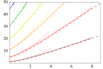
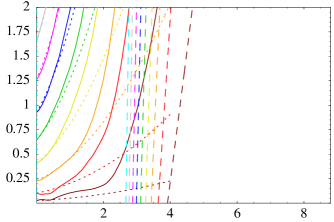
Figure 1: $\Delta S$ vs $g$ for $\beta=16,64,768$ (top to bottom). Resistor color codes indicate $k=1,2,\dotsc,9$. Solid curves: $\Delta S$ obtained by integration of $\Psi_{k}$ calculated from PIMC. Dashed curves: $\Delta S$ evaluated considering only Gaussian fluctuations about winding number trajectories. Dotted curves: $\Delta S$ from perturbation theory about small-$g$ limit, up to $O(g^{2})$. At high temperatures (top), PIMC results agree with the Gaussian approximation in Eq.(23). As temperature is lowered (middle), non-Gaussian fluctuations become important, and significant deviations from the Gaussian approximation are observed. At very low temperatures (bottom), Eq.(23) fails completely.

Figure 2 shows the correlator $C(\tau)$ vs $\tau$. It is possible to identify at least three distinct regimes in the behavior of $C(\tau)$:

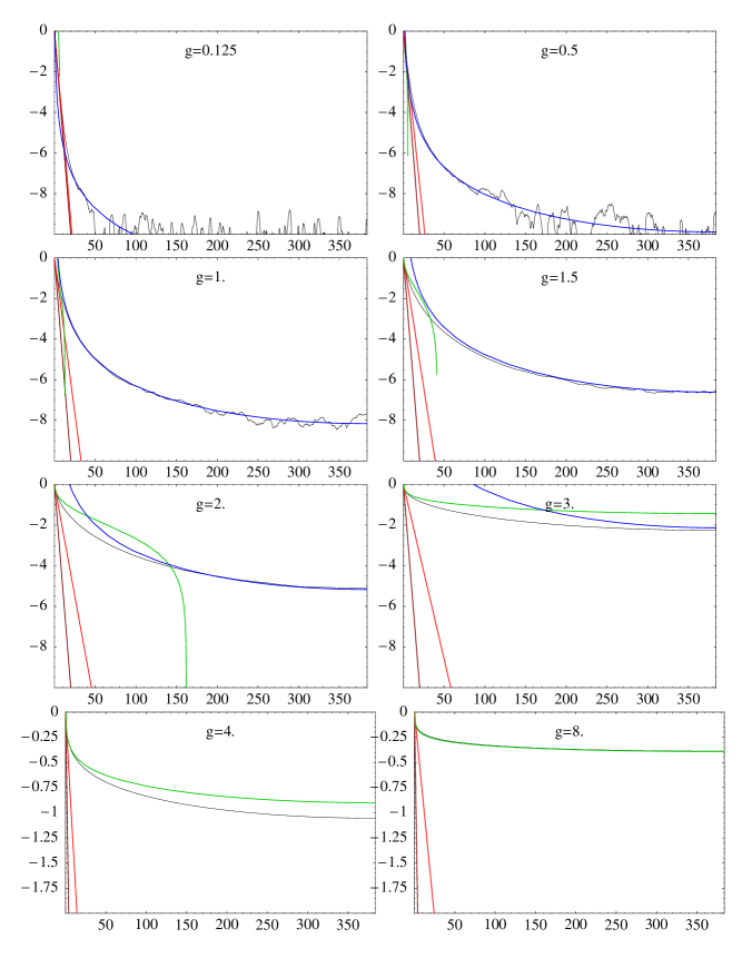
Figure 2: $\ln[C(\tau)]$ vs $\tau$ for $\beta=768$ for various values of $g$. The curves are symmetrical about $\beta/2$. Black curves: PIMC data. Brown: $C^{\text{exp}}$. Red: $C^{\text{renexp}}$. Green: $C^{\text{log}}$. Blue: $C^{\text{alg}}$. Below $e^{-8}$ the data is swamped by Monte Carlo error. For $g\geq 1$, $C(\beta/2)$ evolves logarithmically (green curve) while $\tau T_{*}<1,\,T_{*}=E_{0}/\sqrt{2(e^{\pi g}-1)}$. For $\tau T_{*}\gg 1$, $C(\tau)$ obeys a power-law (blue curve), $C(\tau)=(T/T_{*})^{2}/\sin^{2}(\pi T\tau)$, for any finite value of $g$.

Exponential regime:

For small $g$ and small $\tau$, the ‘kinetic’ term, Eq.(7), dominates, and the system behaves like a free quantum rotor. The correlation function decays exponentially (brown lines in Fig. 2):

$$C^{\text{exp}}(\tau)\approx\exp\left(-E_{0}\tau\right).$$ (29)

For slightly larger $\tau$, theory and numerics suggest exponential decay with a reduced effective $E_{0}$ (red lines):

$$C^{\text{renexp}}(\tau)\approx\exp\left(-\frac{E_{0}\tau}{1+2g/\pi}\right).$$ (30)

The exponential regime is not very relevant in the context of this paper, which is concerned with large $g$.

Logarithmic regime:

As explained in Eq.(17), $C(\tau)$ is logarithmic in the exponentially wide range $\frac{1}{gE_{0}}\ll\tau\ll\frac{1}{gE_{0}}e^{\pi g/2}$. Restoring the correct cutoff in the logarithm,

$$C^{\text{log}}(\tau) =1-\frac{1}{\pi g}\ln\frac{2e^{\gamma}gE_{0}\sin\pi T\tau}{\pi T},$$ (31)

Algebraic regime:

For $\tau\gtrsim\frac{e^{\pi g}}{2e^{\gamma}gE_{0}}$, Eq.(31) becomes negative, indicating complete failure of the approximation. In fact, the numerically-obtained $C(\tau)$ begins falling below $C^{\text{log}}(\tau)$ once $C(\tau)\lesssim 1/2$, as nonzero winding-number trajectories start becoming important. However, this downward trend does not continue indefinitely, but is arrested by an algebraic decay. It turns out that for large $\tau$, the PIMC calculations agree very well with the following prediction of small-$g$ perturbation theory:

$$C^{\text{alg}}(\tau) =\rho(g)\frac{(T/2E_{0})^{2}}{\sin^{2}\pi T\tau},$$ (32)

where the function $\rho(g)$ is equal to

$$\rho(g) =8(e^{\pi g}-1)=8\pi g+4\pi^{2}g^{2}+O(g^{3}).$$ (33)

In fact, in this regime, the individual $C_{k}(\tau)$ themselves are also given by Eq.(32). Thus, although nonzero winding-number trajectories occur in thermodynamic averages with a significant probability, a calculation which ignores them will fortuitously give the right answer.

The $g=2$ and $g=3$ graphs in Fig. 2 clearly show the crossover from the logarithmic regime to the algebraic regime.

Our result in Eq.(32) supports previous findingschakravarty that the long time dynamics $(C(\tau)=(T/T_{*})^{2}/\sin^{2}(\pi T\tau))$ of the Coulomb gas model, such as Eq.(8), is determined by the critical nature of the Ohmic dissipation. This is also confirmed in conformal field theory calculations of the spin correlation function in the Kondo problem.ludwig Further insight comes from Griffiths’ theoremgriffiths2 that at large $\tau$, the correlation function $C(\tau)$ cannot decay faster than the interaction.

Considering a logarithmic law,

$$C(\tau)=1-(1/\pi g)\ln(gE_{0}\tau),$$

for $\tau T_{*}<1$, and a power-law behavior,

$$C(\tau)=(T/T_{*})^{2}/\sin^{2}(\pi T\tau),$$

for $\tau T_{*}>1$, we obtain the impurity susceptibility,

$$\chi_{dc}(T)\approx\chi_{dc}(0)-(2M^{2}/3T_{*})(T/T_{*})^{2},\qquad T\ll T_{*}.$$ (34)

Here $\chi_{dc}(0)$ is exponentially large in $g$, of the order of $\chi_{dc}(T_{*})$ evaluated using Eq.(19).

We also present a few more figures. Figure 3 is a log-log plot of $C(\beta/2)$ vs $\beta$ for various $g$, clearly showing the crossover from the logarithmic regime to the algebraic regime.

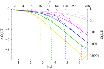
Figure 3: $C(\beta/2)$ vs $\beta$ for $g=0.5,1,1.5,2,3$ (bottom to top). Colors indicate values of $g$. Solid lines are PIMC results. Dotted lines are $C^{\text{log}}(\beta/2)$. Dashed lines are $C^{\text{alg}}(\beta/2)$. A clear crossover from a logarithmic law to a power law can be seen as the temperature is decreased.

Figure 4 is a log-log plot of $\chi(T)$ vs $\beta$ for various $g$, confirming that at exponentially low temperatures the susceptibility saturates at exponentially large values according to Eq. (34). Note that for the larger values of $g$, simulations have not been performed at low enough $T$ to observe saturation. The errors in $\chi(T)$ are smaller than the errors in $C(\beta/2)$ because $\chi$, being an integral, is dominated by the behavior of $C(\tau)$ at small $\tau$, which is less susceptible to MC error.

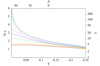
Figure 4: $\chi_{dc}$ vs $T$ for $g=0.125,0.25,0.3,0.5,1,1.5,2,3,4,8$ (bottom to top). The saturation of impurity susceptibility below $T^{*}$ and a $T^{2}$ deviation from saturation can be seen in all but the top three curves, for which $T^{*}$ is extremely small.

Figure 5 is a phase diagram based on the behavior of $C(\beta/2)$ as a function of $g$ and $T$. The dashed and dotted lines represent smooth crossovers rather than phase transitions. Only the $g>1$ part of the phase diagram is relevant to the current paper. The crossover between logarithmic and algebraic behavior occurs at $T^{*}=E_{0}/\sqrt{2(e^{\pi g}-1)}$.

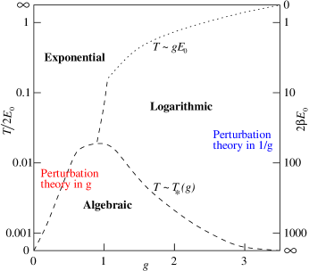
Figure 5: Phase diagram for behavior of $C(\beta/2),\,\beta=1/T$. The algebraic region, $C(\beta/2)=(T/T_{*})^{2}$, occurs at a low enough temperature for any nonzero value of $g$. This phase is dominated by spin-flip processes. Droplet fluctuations are frozen in the logarithmic phase; $C(\beta/2)$ decreases slowly as $1-(1/\pi g)\ln(gE_{0}/T)$. As one approaches criticality (i.e. $g$ increases), spin-flip processes occur below exponentially low temperatures $T<T_{*}=E_{0}/\sqrt{2(e^{\pi g}-1)}$.

VI Discussion

We have studied the paramagnon contribution to the spin correlation function $C(\tau)$ and the static impurity susceptibility $\chi_{dc}(T)$ of a strongly damped $(g>1)$ magnetic defect with $XY$ rotational symmetry in a metal close to a ferromagnetic quantum critical point. Our analysis shows that quantum tunneling (droplet’s spin flip) effects are negligible above an exponentially small temperature, $T_{*}=E_{0}/\sqrt{2(e^{\pi g}-1)}.$ In this regime, $C(\tau)$ and $T\chi_{dc}(T)$ both decrease logarithmically as $T$ decreases. At very low temperatures $T\ll T_{*},$ $C(\tau)$ is very well described by a power law, $C(\tau)=(T/T_{*})^{2}/\sin^{2}(\pi T\tau)$, somewhat analogous to earlier workschakravarty ; ludwig on the Coulomb gas model and equivalent Kondo formulations. The impurity susceptibility $\chi_{dc}(T)$ saturates to an exponentially large but finite value at $T=0$ and does not show any anomalous divergence. Near $T=0$, $\chi_{dc}(T)=\chi_{dc}(0)[1-(2/3)(T/T_{*})^{2}],$ demonstrating the critical nature of the Ohmic dissipation. While our results were obtained for an $XY$ defect, we believe they should be relevant to defects with full spherical symmetry (possibly with additional modifications due to the Berry phase). We stress that there is a qualitative difference between the cases of Isingyuval and $XY$ symmetry due to the critical nature of the long-ranged $1/\tau^{2}$ interaction for one-dimensional (meaning one-time dimension) ferromagnetic chains.kosterlitz

We considered in this paper the action of Eq.(8) and associated non-perturbative effects associated with spin flips. These effects are dominant if, due to the large ferromagnetic polarizability of the host metal, the corrections proportional to $g$ (corresponding to the even powers of exchange coupling $J$) are larger than other Kondo corrections proportional to odd powers of $Jn(\epsilon_{F})$. As analyzed by Larkin and Melnikovlarkin the condition to neglect odd-power Kondo corrections is $g>Jn(\epsilon_{F})$. Since we consider $g>1$, it is sufficient to require just $Jn(\epsilon_{F})>(1+F_{a})^{1/2}$, while the above condition $g>Jn(\epsilon_{F})$ is satisfied trivially for $Jn(\epsilon_{F})\ll 1$.

The weak coupling case $(g\ll 1)$ is analogous to the overcompensated Kondo problem studied by Nozieres and Blandin,nozieres and Abrikosov and Migdalabrikosov where the number of conduction electron channels $N_{ch}$ coupling to the defect is much larger than $2S$. Each conduction electron channel corresponds to a different orbital quantum number. The coupling constant $(Jn_{F})$ obeys the scaling equation

$$\frac{d(Jn_{F})}{d\ln D}=-(Jn_{F})^{2}+N_{ch}(Jn_{F})^{3}+c(Jn_{F})^{4}\cdots,$$ (35)

where $D$ is the bandwidth, and $c$ depends on $S$ but not on $N_{ch}$. The first term in Eq.(35) depends on the sign of the exchange interaction $J$, and for $J>0$ gives rise to the conventional antiferromagnetic Kondo effect with a Kondo temperature $T_{K}=D\exp(-1/Jn_{F})$. The second term describes the scattering of a conduction electron from the impurity dressed by a number $N_{ch}$ of closed electron loops. If the second term is much larger than the first, the coupling constant renormalizes towards zero as follows:

$$J(D)=\frac{J_{0}}{\sqrt{1+\frac{N_{ch}(J_{0}n_{F})^{2}}{2}\ln(D_{0}/D)}}.$$ (36)

The above scaling is the same as the renormalization of $g=(\pi/2)(SJn_{F})^{2}/(1+F_{a})$ obtained by Larkin and Melnikovlarkin for $g\ll 1$ by summing over parquet diagrams:

$$g(T)=\frac{g}{1+\frac{2g}{\pi S^{2}}\ln(E_{0}/T)}.$$ (37)

A comparison of Eq.(35) and Eq.(37) shows that the number of channels is $N_{ch}=2/(1+F_{a})$. As the running coupling constant decreases, the usual first Kondo term in Eq.(35) may no longer be disregarded. If $J>0$ (antiferromagnetic), $J(D)$ flows towards a stable multi-channel Kondo fixed point given by

$$J_{*}n_{F}=1/N_{ch}=(1+F_{a})/2,$$ (38)

which corresponds to a Kondo temperature

$$T_{K}=E_{0}e^{-1/J_{*}n_{F}}=E_{0}e^{-2/(1+F_{a})}.$$ (39)

If $J<0$ (ferromagnetic), the coupling constant scales to zero. In that case, as in the ferromagnetic Kondo problem, the impurity’s susceptibility is expected to obey a Curie-Weiss law as $T\rightarrow 0$.

In this paper we have considered $g>1$, and perturbation theory in $1/g$ also shows that $g$ flows towards zero,others as is evident from Eq.(16). Thus, in both the weak-coupling ($g<1$) and the strong-coupling ($g>1$) cases, $g$ is renormalized towards zero until very low temperatures below $T_{K}=E_{0}\exp[-2/(1+F_{a})]$, when odd-power terms of the coupling $J$ become relevant.

The overall picture emerging from our analysis is that the compensation of the droplet’s moment takes place in two basic stages. In the first stage, on which we focus in the main text, the paramagnon fluctuations, which originally enhance a spin $S$ to the large magnetic moment $M$, are gradually stripped off. This quenching of the droplet moment takes place below the temperature $T_{*}$, which in our case is given by $T_{*}\approx E_{0}\exp[-\pi g/2]=E_{0}\exp[-(\pi SJn_{F}/2)^{2}/(1+F_{a})].$ At the second stage, and an even lower temperature $T_{K}$, for $J>0$ the usual Kondo effect compensates the remaining moment leading to a multi-channel Kondo fixed point, while for $J<0$, the impurity spin becomes free. The multi-channel Kondo fixed point could be an artifact of our assuming equal coupling of the droplet to all the $N_{ch}$ angular momentum channels of the conduction electrons. In reality, the coupling for each channel may be different, and it is possible that the impurity spin will get compensated successively in different channels. Maebashi, Miyake, and Varmavarma recently analyzed the problem in the Kondo regime and concluded from the scaling equations that the coupling constants approach a multi-channel Kondo fixed point. They also suggested that at unattainably low temperatures a crossover happens when a single channel wins out. In the last stages of preparation and submission of our manuscript we became aware of another workvojta which arrived to some conclusions similar to ours in the case of $O(N)$ spin symmetry in the large-$N$ limit.

In this paper we considered a dilute system of impurities, so that mutual interaction among impurities can be neglected. The size of a magnetic droplet, $L$, is determined by the dispersion relation of the paramagnon modes and the proximity to the critical point, as $L\sim\xi_{0}/\sqrt{1+F_{a}}$. As the quantum critical point is approached, the size of the droplets grows, and the system can be considered dilute only if the density of impurities is $n_{imp}\ll\xi_{0}^{-3}(1+F_{a})^{3/2}$. We also ignore various anomalous effects which possibly arise in very close proximity to the critical point,belitz and explore only the nearly ferromagnetic Fermi-liquid regime.

There are several experimental systems, involving impurities with giant magnetic moments in a nearly ferromagnetic host metal, in which it may be possible to study magnetic droplet phenomena systematically.korenblit Among these are iron ($Fe$) dissolved in various transition metal alloys,clogston nickel ($Ni$) impurities in palladiumshaltiel ; loram1 ($Pd$), and cobalt ($Co$) impurities in a platinum ($Pt$) host.shen

There are some close connections between the dynamics of a magnetic moment with $XY$ symmetry and the dynamics of the electromagnetic phase in quantum dots and granular metals. The power law behavior of $C(\tau)$ at long-$\tau$ (or small temperatures) can be associated with inelastic cotunneling in the literature of mesoscopic physics.averin Inelastic cotunneling was long understood to be important at low temperature $(T<E_{0}\ln(g^{-1}))$ for weak inter-grain coupling $(g<1)$. Our present work shows that this is so even when inter-grain coupling is large, the difference being that when $g>1$, inelastic cotunneling becomes important only at exponentially low temperatures $T<T_{*}$. The competition of inelastic cotunneling and the Coulomb blockade can lead to interesting consequences for the transport properties of a granular metal.loh

- (1) A.I.Larkin and V.I.Melnikov, Sov. Phys. JETP 34, 656 (1972).
- (2) S.Doniach and S.Engelsberg, Phys. Rev. Lett. 17, 750 (1966).
- (3) A.J.Millis, D.K.Morr, and J.Schmalian, Phys. Rev. Lett. 87, 167202 (2001).
- (4) In ignoring spin flips for the case, Millis et al.millis1 relied on the conclusions of W.Zwerger, A.T.Dorsey, and M.P.A.Fisher, Phys. Rev. B 34, 6518 (1986). There the authors studied the quantum dynamics of a resistively shunted Josephson junction and found that dissipation completely suppresses winding numbers (spin-flips in our paper). The model we consider in Eq.(8) differs from Zwerger et al., for the dissipation naturally couples to the magnetization, , and not to the angular velocity . For the action in Eq.(8) we find non-zero winding numbers are not suppressed.
- (5) A.H.Castro-Neto, G.Castilla, and B.A.Jones, Phys. Rev. Lett. 81, 3531 (1998); A.H.Castro-Neto and B.A.Jones, Phys. Rev. B 62, 14975 (2000).
- (6) R.B.Griffiths, Phys. Rev. Lett. 23, 17 (1969).
- (7) B.M.McCoy and T.T.Wu, Phys. Rev. 176, 631 (1968); B.M.McCoy, Phys. Rev. B 2, 2795 (1970).
- (8) A.Schröder et al., Nature 407, 351 (2000).
- (9) Q. Si et al., Nature 413, 804 (2001).
- (10) P.W.Anderson, Phys. Rev. 124, 41 (1961).
- (11) For a review of the Anderson model and the Kondo problem, see A.C.Hewson, The Kondo Problem to Heavy Fermions (Cambridge University Press) (1993).
- (12) T.Moriya, Spin Fluctuations in Itinerant Electron Magnetism (Springer series in solid-state sciences; 56), Springer-Verlag Berlin Heidelberg (1985).
- (13) V. Ambegaokar et al., Phys. Rev. Lett. 48, 1745 (1982).
- (14) S.E. Korshunov, JETP Lett 45, 434 (1987).
- (15) G.Falci, G.Schön, and G.T.Zimanyi, Phys. Rev. Lett. 74, 3257-3260 (1995).
- (16) E.Bascones, C.P.Herrero, F.Guinea, and G.Schön, Phys. Rev. B 61, 16778 (2000).
- (17) C.P. Herrero, G.Schön, and A.D. Zaikin, Phys. Rev. B 59, 5728 (1999).
- (18) R.M. Neal, Probabilistic Inference Using Markov Chain Monte Carlo Methods, Technical Report CRG-TR-93-1, Dept. of Computer Science, University of Toronto (1993).
- (19) D.J.C. MacKay, Information Theory, Inference, and Learning Algorithms (Cambridge University Press) (2003).
- (20) D.M.Ceperley, Rev. Mod. Phys. 67, 279-355 (1995).
- (21) W. Zwerger, M. Scharpf, Zeitschrift Phys. B 85, 421 (1991), S.Chakravarty and J.Rudnick, Phys. Rev. Lett. 75, 501 (1995).
- (22) A.W.W.Ludwig and I.Affleck, Nucl. Phys. B428[FS], 545 (1994).
- (23) R.B.Griffiths, J. Math. Phys. (N.Y.) 8, 478 (1967); 8, 484 (1967); for the discussion of the symmetry see J. Ginibre, Commun.Math.Phys. 16, 310 (1970).
- (24) P.W. Anderson, G. Yuval, and D.R. Hamann, Phys. Rev. B 1, 4464 (1970); P.W. Anderson and G. Yuval, J. Phys. C 4, 607 (1971).
- (25) J.M. Kosterlitz, Phys.Rev.Lett. 37, 1577 (1976).
- (26) P. Nozieres, A. Blandin, J. de Physique 41, 193 (1980).
- (27) A.A. Abrikosov, A.A. Migdal, J.Low Temp.Phys. 3, 519 (1970).
- (28) The renormalization in Eq.(16) has been obtained in different context in numerous earlier works. See for instance, G.Falci et al.,falci95 and references therein.
- (29) H.Maebashi, K.Miyake, and C.M.Varma, Phys. Rev. Lett. 88, 226403 (2002).
- (30) T.Vojta and J.Schmalian, cond-mat/0405609.
- (31) S. Misawa, Journal of Phys. Soc. of Japan 68, 32 (1999), D. Belitz, T.R. Kirkpatrick, and T.Vojta, Phys.Rev.Lett. 82, 4707 (1999).
- (32) For a review, see I.Ya Korenblit and E.F.Shender, Uspekhi Fiz. Nauk 126, 233 (1978).
- (33) A.M.Clogston, B.T.Matthias, M.Peter, H.J.Williams, E.Corenswit, and R.C.Sherwood, Phys. Rev. 125, 541 (1962).
- (34) D. Shaltiel, J.H. Wrenick, H.J. Williams, Phys. Rev. 135, 1346 (1965).
- (35) J.W.Loram and K.A.Mirza, J. Phys. F 15, 2213 (1985); J.W.Loram, K.A.Mirza, and Z.Chen, J. Phys. F 16, 233 (1986).
- (36) L.Shen, D.S.Schreiber, A.J.Arko, Phys. Rev. 179, 512 (1969).
- (37) M.Jutzler, Z. Phys. B - Cond. Matt. 64, 115 (1986).
- (38) D.V. Averin, Yu.V. Nazarov, Phys.Rev.Lett. 65, 2446 (1990).
- (39) V.Tripathi, M.Turlakov, Y.L. Loh, J. Phys.: Condens. Matter 16, 1 (2004).