Self-consistent local GW method: Application to $3d$ and $4d$ metals

Abstract

Using the recently developed version of the GW method employing the one-site approximation and self-consistent quasiparticle basis set we calculated the electronic structure of $3d$ and $4d$ transition metals at experimental atomic volumes. The results are compared with traditional local density approach and with experimental XPS and BIS spectra. Our results indicate that this technique can be used as a practical starting point for more sophisticated many-body studies of realistic electronic structures.

I Introduction

The electronic properties of many solids are described reasonably well in the local density approximation (LDA) of the density functional theory (DFT),DFT which is essentially a single-particle theory representing a cardinal simplification of the original many-body problem. However, the LDA becomes inadequate in materials exhibiting strong spatial correlations between different electrons in atoms with localized orbitals, temporal correlations (retardation) associated with Coulomb screening, etc. The corresponding difficulties are extremely hard to overcome within the DFT without sacrificing the first-principles approach.

One of the methods used to correct the deficiencies of LDA in the description of excited states in metals and semiconductors is the GW approximation (GWA).Hedin ; AG-rev The GWA usually improves the band gaps in semiconductors and insulators;AG-rev in metals it may provide information on the quasiparticle lifetimes and renormalization which is absent in the DFT.AG-rev ; Echenique However, in all treatments used until recently, the GWA was employed in a non-self-consistent fashion, by using unrenormalized Green’s functions based on the Kohn-Sham wave functions obtained in LDA. Such an approach is easier to implement, but it is internally inconsistent, does not correspond to any Luttinger-Ward functionalLW and hence violates basic conservation laws,Baym and produces different results depending on the approximation used to solve the Kohn-Sham equations. On the other hand, studies of the homogeneous electron gas have shown that GW self-consistency worsens the agreement with experiment at typical metallic densities,Holm highlighting the limitations of GWA which is strictly correct only in the high-density limit.

Recently, two self-consistent realizations of the Green’s function method were demonstrated. One of themZA was tailored for transition metals and employed the one-site approximation for the self-energy which is based on the assumption that dynamical screening in $d$-metals is well described at the intraatomic level. Some spin-selective diagrams beyond the GW set were also included. The results for Fe and Ni were quite reasonable, although no improvement was obtained compared to LDA. While the choice of GW diagrams is unjustified for the homogeneous electron gas at typical metallic densities and likewise for semiconductors (the diagrams that are left out do not contain any small parameter), it was noted that the situation may be better in transition metals, because high orbital degeneracy provides an additional enhancement to the diagrams with the largest number of closed electron loops favoring the GW set.ZA In addition, for transition metals the “local” (one-site) approximation for the self-energy is quite reasonable due to the short screening length and greatly facilitates self-consistent calculations.

Another realizationKE using GW set with the full $\mathbf{k}$-dependence of the self-energy was applied to elemental semiconductors. It was found that self-consistency and accurate treatment of core electrons improve the agreement with experiment for the band gaps in Si and Ge.

While the adequacy of GWA for the studies of metals and semiconductors has not been firmly established from the point of view of the many-body theory, this method may be regarded as one of the possible steps toward a consistent Green’s function-based scheme. Therefore, it is important to establish the accuracy of this approximation for different materials, and in particular for transition metals where, as noted above, there are reasons for it to work better than in the homogeneous electron gas. To this end, in this paper we calculate the conduction-band spectra for all elemental $3d$ and $4d$ metals using the self-consistent GW approach of Ref. ZA, and compare them with the observed ones and with those given by the LDA.

II Self-consistent GW method

The technique used in this paper was introduced in Ref. ZA, . Here we describe some points in more detail.

The self-energy $\Sigma=\delta\Phi/\delta G$ is obtained from the Luttinger-Ward generating functional $\Phi$ defined by the set of skeleton graphs. LW The Hartree diagram gives the local contribution $V_{\mathrm{H}}(\mathbf{r})$, and the exchange diagram contributes $\Sigma_{x}=V(\mathbf{r}-\mathbf{r}^{\prime})\int\mathrm{Im}G(\mathbf{r},\mathbf{r}^{\prime},\epsilon)d\epsilon/\pi$ where $V$ is the Coulomb potential. The total contribution of the remaining GW sequence (the “correlation term”) is

$$\Sigma_{c}(\mathbf{r},\mathbf{r}^{\prime},\epsilon) = -\int G(\mathbf{r},\mathbf{r}^{\prime},\epsilon-\omega)V(\mathbf{r}-\mathbf{r}_{1})$$ (1)

$$\times \Pi(\mathbf{r}_{1},\mathbf{r}_{2},\omega)W(\mathbf{r}_{2},\mathbf{r}^{\prime},\omega)\,d\mathbf{r}_{1}\,d\mathbf{r}_{2}\,\frac{d\omega}{2\pi i}$$

Here $W$ is the effective (screened Coulomb) interaction defined by the integral Dyson equation

$$W=V-\int V(\mathbf{r}-\mathbf{r}_{1})\Pi(\mathbf{r}_{1},\mathbf{r}_{2},\epsilon)W(\mathbf{r}_{2},\mathbf{r}^{\prime},\epsilon)d\mathbf{r}_{1}d\mathbf{r}_{2}$$ (2)

and the polarization operator

$$\Pi(\mathbf{r},\mathbf{r}^{\prime},\omega)=\int G(\mathbf{r},\mathbf{r}^{\prime},\epsilon)G(\mathbf{r}^{\prime},\mathbf{r},\epsilon+\omega)d\epsilon.$$ (3)

Contour of integration in Eqs. (1),(3) is directed along the imaginary axis and embraces the cut on the real axis from the Fermi energy $E_{F}$ to the external energy. The GW approximation may be modified by the inclusion of vertex corrections in the polarization operator (3) which may improve the results in some cases.

The calculations are drastically simplified by the use of the one-site approximation ZA (OSA), in which the self-energy is calculated only on one lattice site neglecting all non-diagonal maxrix elements connecting different lattice sites. Thus, in OSA the self-energy depends on energy and on the coordinates $\mathbf{r}$, $\mathbf{r}^{\prime}$ belonging to the same unit cell. In order to implement OSA we first need to choose an appropriate on-site basis. Inspired by the good description of the band structure of densely packed solids achieved in the atomic sphere approximation within the linear muffin-tin orbital method (LMTO-ASA), we used a very similar, minimalistic approach. For the basis set we also use just one function per each angular momentum $l$ and its projection $m$ (below we denote $L\equiv lm$), along with its energy derivative. The radial basis functions $\phi_{l}(r)$ satisfy the “Schrödinger-type” equation

$$\left[\epsilon_{l}+\frac{\Delta_{l}}{2}-V_{\mathrm{H}}-\widehat{\Sigma}_{l}(\epsilon_{l})\right]\phi_{l}(r)=0$$ (4)

where $\Delta_{l}$ is the radial part of the Laplasian, and $\widehat{\Sigma}_{l}$ is an integral radial operator whose kernel is obtained from $\mathop{\mathrm{Re}}\widehat{\Sigma}$ by projecting onto the $l$ subspace:

$$\Sigma_{l}(r,r^{\prime},\epsilon)=\frac{1}{2l+1}\sum\limits_{m}\int Y_{L}(\hat{r})\mathop{\rm Re}\Sigma_{xc}(\mathbf{r},\mathbf{r}^{\prime},\epsilon)Y_{L}(\hat{r}^{\prime})dodo^{\prime}$$ (5)

where we denoted $\Sigma_{xc}\equiv\Sigma_{x}+\Sigma_{c}$, $Y_{L}$ are the spherical harmonics, and integration is over the directions of $\mathbf{r}$,$\mathbf{r}^{\prime}$. The operator $\widehat{\Sigma}_{l}$ may be represented as the sum of a local part $\Sigma_{l}^{(l)}(r)$ similar to an external potential and a nonlocal part $\widehat{\Sigma}_{l}^{(n)}$ which (after acting on $\phi_{l}$) gives a linear combination of $\phi_{l^{\prime}}$ with $l^{\prime}\neq l$.

Similarly to the LMTO-ASA method, the solutions of Eq. (4) are only found at one energy $\epsilon_{l}$ for each $l$ which is fixed at the center of gravity of the corresponding band. We may safely discard the imaginary part of the self-energy operator because it is small in the vicinity of $E_{F}$ where $\epsilon_{l}$ is usually chosen. Thus, our radial basis functions are real. The non-local equation (4) is solved by iterations. If $\phi_{l}^{n}$ is the solution after $n$ iterations, then the solution on iteration $n+1$ is obtained using auxiliary functions $f_{l}$ and $g_{l}$ defined as

$$\left[\epsilon_{l}+\frac{\Delta_{l}}{2}-V_{\mathrm{H}}-\Sigma_{l}^{(l)}(r)\right]f_{l}(r) = \widehat{\Sigma}_{l}^{(n)}(\epsilon_{l})\phi_{l}^{n},$$ (6)

$$\left[\epsilon_{l}+\frac{\Delta_{l}}{2}-V_{\mathrm{H}}\right]g_{l}(r) = 0$$ (7)

according to $\phi_{l}^{n+1}(r)=f_{l}(r)+A\,g_{l}(r)$, where the coefficient $A$ is found by normalizing $\phi_{l}^{n+1}$. Just as in the LMTO method, in addition to $\phi_{l}$ we compute its energy derivative $\dot{\phi}_{l}\equiv\partial\phi_{l}/\partial\epsilon$:

$$\left[\epsilon_{l}+\frac{\Delta_{l}}{2}-V_{\mathrm{H}}-\widehat{\Sigma}_{l}(\epsilon_{l})\right]\dot{\phi}_{l}=-\phi_{l}+\frac{\partial\widehat{\Sigma}_{l}(\epsilon_{l})}{\partial\epsilon_{l}}\phi_{l}$$ (8)

To stabilize the solution of the Schrödinger equation (4), we added the exchange with the nearest-neighbor cells to $\Sigma_{xc}$. The corresponding matrix element was subtracted from Green’s function (9) below.

With the on-site self-energy $\Sigma_{xc}(\mathbf{r},\mathbf{r}^{\prime},\epsilon)$ defined for $r,r^{\prime}$ within the single unit cell we can calculate its matrix elements between the muffin-tin “eigenfunctions” $\chi_{\mathbf{k}\nu}$, which in turn are the linear combinations of $\phi_{l}$ and $\dot{\phi}_{l}$. Due to the $\mathbf{k}$-dependence of $\chi_{\mathbf{k}\nu}$ the self-energy also acquires $\mathbf{k}$-dependence, just as the local potential in LDA. Finally, on-site Green’s function is found by integration using the tetrahedron method:

$$G({\bf r,r^{\prime}},\varepsilon)=\sum_{{\bf k}\nu}\frac{\chi_{\mathbf{k}\nu}^{R}({\bf r})\chi_{\mathbf{k}\nu}^{L*}({\bf r^{\prime}})}{\varepsilon-\lambda_{\mathbf{k}\nu}}$$ (9)

where $\chi_{\mathbf{k}\nu}^{R}$ and $\chi_{\mathbf{k}\nu}^{L}$ are right and left eigenvectors, and $\lambda_{\mathbf{k}\nu}$ the eigenvalues of the non-Hermitian operator $H_{0}+\Sigma_{xc}$ where $H_{0}$ is the Hartree Hamiltonian. Eq. (9) imposes the locality condition and is equivalent to the self-consistency condition of the dynamical mean-field theory.DMFT

III Conduction band spectra of transition metals

Using the technique described above (below referred to as “GW”) we calculated the spectral densities $N(\epsilon)=\mathop{\mathrm{Tr}}\mathop{\mathrm{Im}}G(\epsilon)$ for elemental $3d$ and $4d$ metals, where LDA has long been the only appropriate approximation. We used the fcc structure for hcp elements (Sc, Ti, Y, Zr, Tc, Ru, Co) and the bcc structure for Mn. All atomic volumes were taken from experiment. Cr was treated within the single bcc cell, and hence was non-magnetic.

The iterations were started from the LDA potential, and at each iteration the non-local self-energy was mixed to this potential with a gradually increasing weight, so that in the end only $\Sigma_{xc}$ was left. In the final state the magnitude of $\Sigma_{xc}$ differs by about 40% from its initial value based on the LDA wave functions. The iterational procedure is rather stable in all metals except Ni where the magnetic moment is very sensitive to the details of the calculation.

The results are shown in Figs. 1,2 along with the LDA densities of states (DOS) and the experimental XPS and BIS spectra taken from Refs. XPS, ; BIS, . Strictly speaking, comparison with experiment requires the calculation of the corresponding matrix elements, but we believe that in the present context some qualitative conclusions can be drawn based on the spectral densities.

The main differences between the LDA DOS and GW spectral density may be summarized as follows. The conduction band widens as all DOS features are pushed away from $E_{F}$; this outward shift is roughly proportional to the distance from $E_{F}$. Moreover, all DOS features are increasingly smeared out due to the decreasing quasiparticle lifetime as the distance from $E_{F}$ increases. Substantial spectral weight is transferred from the quasiparticle states to the incoherent “tail” extending far below $E_{F}$.

The LDA DOS for $d$-metals is typically too small to account for experimentally measured electronic specific heat $C=\gamma T$. As seen from Figs. 1,2, the GW spectral density at $E_{F}$ is generally smaller compared to LDA. Although to obtain $\gamma$ we have to remove the renormalization factor $Z$ from $\mathop{\mathrm{missing}}{Im}G$, the GW method does not improve the overall agreement with $\gamma$ measurements.

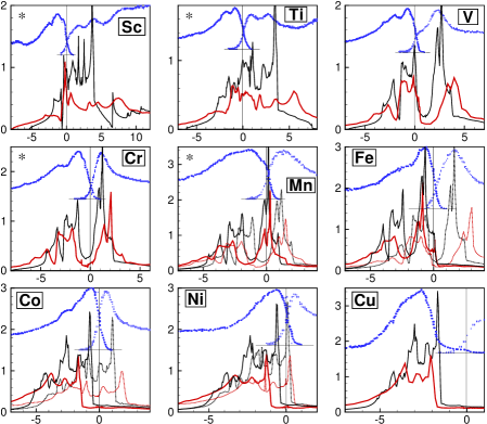
Figure 1: Spectral densities obtained in GW-OSA (red lines), LDA densities of states (black lines), and experimental XPS and BIS spectra (blue dotted lines shifted up) for $3d$ metals. For magnetic elements the calculated curves for majority-spin and minority-spin electrons are plotted in solid and dotted lines, respectively. Elements for which the crystal structure was not experimental (including Cr) are marked by a star in the upper left corner of the graph. In all graphs the $x$ axis shows energy referenced from $E_{F}$ in eV, and the $y$ axis denotes the spectral density in eV^-1 for the calculated curves.

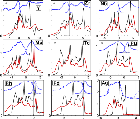
Figure 2: Same as Fig. 1 but for $4d$ metals.

The differences between the GW and LDA spectra are most notable for early transition metals (treated here in the fcc structure) where the strongest unoccupied peaks given by LDA are almost completely smeared out in GW. Notably, the worst agreement with experiment for the LDA spectra is observed for the same elements. In particular, the position of the Fermi level obtained in LDA for hcp Sc and Y appears to be off by nearly 1 eV.XPS

The agreement between LDA and GW improves as we progress to later transition metals and as the fcc structure is replaced by the bcc one. Already in V and Nb the GW and LDA curves are quite similar except for the shift of the unoccupied $d$-peak by 1.5–2 eV to higher energies.

As in LDA, the $3d$ metals from Mn to Ni were magnetic in our calculation. For simplicity, we used the bcc structure for Mn, and also the fcc structure for Co (this structure is often realized in thin films). As it is seen from Fig. 1, the general features of the GW spectral density described above are observed in these metals as well. In general, the GW description also gives a reasonable exchange splitting and magnetic moment. We obtained the moments of 0.9 $\mu_{B}$ for Mn compared to 1.03 $\mu_{B}$ in LDA, 2.3 $\mu_{B}$ for Fe compared to 2.25 $\mu_{B}$ in LDA, and 1.85 $\mu_{B}$ for fcc Co compared to 1.62 $\mu_{B}$ in LDA. From these results it is clear that there is no systematic trend for GW to give larger or smaller magnetic moments compared to LDA. The magnetic moment in Ni is rather sensitive to various details of the calculation, and proper convergence turned out to be problematic. We believe that the approach based on Matsubara Green’s functions is necessary to stabilize this problem. Apart from the exchange splitting, the shape of the spectrum is quite stable. We also note that the magnetic moment is expected to be sensitive to the choice of the skeleton graph set.

As an example of the general trend of band dilatation off the Fermi level, the distance from $E_{F}$ to the upper edge of the fully occupied $d$-band in Cu and Ag is notably larger in GW compared to LDA, which results in a better agreement with experimental XPS spectra. On the other hand, we also observe a rather strong upward shift of the unoccupied peak in V, Nb, Fe and Mo in obvious disagreement with the BIS spectra. This shift is more pronounced compared to the downward shift of the occupied states at a similar distance from $E_{F}$.

The results presented above demonstrate that self-consistent GF approach with one-site approximation can be used for ground state studies. For $3d$ and $4d$ systems we have shown that the GW spectral density is generally similar to the LDA density of states, while the GF approach includes typical Fermi-liquid effects such as finite quasiparticle lifetime and self-consistent renormalization. The preliminary comparison with experiment is rather satisfactory and clearly indicates the problems that need improvement beyond our simple GW-OSA technique are similar to those in LDA — the exchange splitting in ferromagnets, value of $N(E_{F})$, and the unoccupied peak position which is too high for some metals. In general, the presented technique based on the Luttinger-Ward functional is a practical alternative to other methods based on the density functional theory and can serve as a reliable starting point for more sophisticated methods..

This work was carried out at the Ames Laboratory, which is operated for the U.S. Department of Energy by Iowa State University under Contract No. W-7405-82. This work was supported by the Director for Energy Research, Office of Basic Energy Sciences of the U.S. Department of Energy. NEZ acknowledges support from the Council for the Support of Leading Scientific Schools of Russia under grant NS-1572.2003.2.

References

- (1) P. Hohenberg and W. Kohn, Phys. Rev. 136, B864 (1964); W. Kohn and L.J. Sham, Phys. Rev. 140, A1133 (1965).
- (2) L. Hedin, Phys. Rev. 139, A796 (1965)
- (3) F. Aryasetiawan and O. Gunnarsson, Rep. Prog. Phys. 61, 237 (1998).
- (4) V.M. Silkin, E.V. Chulkov, and P.M. Echenique, Phys. Rev. B 68, 205106 (2003); see also references in this paper.
- (5) J.M. Luttinger and J.C. Ward, Phys. Rev. 118, 1417 (1960).
- (6) G. Baym and L.P. Kadanoff, Phys. Rev. 124, 287 (1961); G. Baym, Phys. Rev. 127, 1391 (1962).
- (7) B. Holm and U. von Barth, Phys. Rev. B 57, 2108 (1998).
- (8) N.E. Zein and V.P. Antropov, Phys. Rev. Lett. 89, 126402 (2002).
- (9) W. Ku and A.G. Eguiluz, Phys. Rev Lett. 89, 126401 (2002).
- (10) A. Georges, G. Kotliar, W. Krauth and M. Rozenberg, Rev. Mod. Phys. 68, 13 (1996).
- (11) N.E. Bickers and D.J. Scalapino, Ann. Phys. (N.Y.) 193, 206 (1989).
- (12) F. Aryasetiawan, T. Miyake and K. Terakura, Phys. Rev. Lett. 88, 166401 (2002).
- (13) A.G. Narmonev and A.I. Zakharov, Phys. Met. Metall. 65, 315 (1988).
- (14) W. Speier et al., Phys. Rev. B 30, 6921 (1984).