The Effects of Phase Separation in the Cuprate Superconductors

Abstract

Phase separation has been observed by several different experiments and it is believed to be closely related with the physics of cuprates but its exactly role is not yet well known. We propose that the onset of pseudogap phenomenon or the upper pseudogap temperature $T^{*}$ has its origin in a spontaneous phase separation transition at the temperature $T_{ps}=T^{*}$. In order to perform quantitative calculations, we use a Cahn-Hilliard (CH) differential equation originally proposed to the studies of alloys and on a spinodal decomposition mechanism. Solving numerically the CH equation it is possible to follow the time evolution of a coarse-grained order parameter which satisfies a Ginzburg-Landau free-energy functional commonly used to model superconductors. In this approach, we follow the process of charge segregation into two main equilibrium hole density branches and the energy gap normally attributed to the upper pseudogap arises as the free-energy potential barrier between these two equilibrium densities below $T_{ps}$. This simulation provides quantitative results in agreement with the observed stripe and granular pattern of segregation. Furthermore, with a Bogoliubov-deGennes (BdG) local superconducting critical temperature calculation for the lower pseudogap or the onset of local superconductivity, it yields novel interpretation of several non-conventional measurements on cuprates.

I Introduction

The existence of the pseudogap in all family of high-temperature superconductors (HTSC) has been verified by several different experimental techniques as discussed by many reviewsTS ; Tallon . As a consequence of many years of scientific effort, there is a solid consensus of its existence at least in the underdoped regime. On the other hand, there is currently no agreement on such basic facts as to its nature and origin. After its discoveryAlloul ; Tallon , it was realized that some experiments detected the pseudogap temperature $T^{*}$ at very high values while others would place it just above the critical temperature $T_{c}$. This is probably because different probes are able to detect different properties but, the fact is that this large discrepancy triggered a variety of different proposals. Just to mention a few ideas and works; Emery et al.Emery called the high $T^{*}$ as $T_{1}^{*}$, the crossover temperature at which charge inhomogeneities become well defined and the low $T^{*}$ as $T_{2}^{*}$ and associated it with a spin gap and they both merged into $T_{c}$ at the slightly overdoped region of the phase diagram. In their review Timusk and StattTS also presented a similar phase diagram but they related the lower pseudogap temperature to $T^{*}$ and the upper one also to a crossover temperature $T_{1}^{*}$. The lower and the higher $T^{*}$ were also considered as the opening of a spin and a charge gap respectivelyMKZD . The lower $T^{*}$ was also attributed to superconducting phase fluctuationsEK and many different experiments claimed to have detected such fluctuationsCorson ; Bernhard ; Xu ; Wang ; Meingast . Thus the existence of the two pseudogaps in the cuprates has been compiled by several worksTS ; Tallon ; Markiewicz as the result of many different data. In fact, analyzing the data from angle-resolved photoemission (ARPES) and angle-integrated photoemission (AIPES), Ino et al.Ino could distinguish not two but three different energy scales.

Another controversial point is whether the pseudogap and the superconducting gap have the same origin or not. Tunneling spectroscopyRenner ; Miyakawa ; Suzuki seems to show that the gap evolves continuously from the superconducting into the normal phase without any anomaly, suggesting that the pseudogap and superconducting gaps have the same origin. The common origin was also supported by some ARPESHarris and scanning tunneling spectroscopy (STM)Kugler data. Muon spin rotating experimentsUemura characterized $T^{*}$ as the pair formation line in agreement with the fluctuation theories of pre-formed superconducting pairsEmery ; EK ; Pieri . These STM and ARPES experiments have also measured the pseudogap in the overdoped region in opposition to many othersTS ; Tallon ; Uemura which the pseudogap temperature line appears to fall a little beyond the optimum doping value. On the other hand, intrinsic (c-axis interplane) tunneling spectroscopyKrasnov00 ; Krasnov ; Yurgens led to results against a superconducting origin of the pseudogap what was also confirmed by the same type of experiment in high magnetic fieldKrasnov . This conclusion, against the common origin of the pseudogap and superconducting gap, is also shared by Tallon and Loram after the analysis of data from many different experimentsTallon .

The above resumed paragraphs intended to show that, despite the enormous experimental effort after all these years, there are still some basic open questions in this field. These open questions motivated us to make the present novel work which connects the large pseudogap $T^{*}$ to the onset of phase separation. There is now considerable evidence that the tendency toward phase separation or intrinsic hole clustering formation is an universal feature of doped cupratesMuller ; Castro ; Statt ; CEKO ; Wang2 . Phase separation in hole rich and hole poor regions was theoretically predictedZaanen and has been observed in the form of stripesTranquada ; Bianconi and in the form of microscopic grains or mesoscopic segregation by STM measurementsPan ; Davis . Although the STM results has been questioned as a surface phenomena which does not reflect the nature of the bulk electronic stateLoram , the inhomogeneities has also been seen by neutron diffractionTranquada ; Bianconi ; Buzin which is essentially a bulk type probe in underdoped and optimally doped region of the $La_{2-x}Sr_{x}CuO_{4}$ phase diagram. Another bulk-type measurement using nuclear quadrupole resonance (NQR)Singer has observed an increase in the hole density spatial variation of $La_{2-x}Sr_{x}CuO_{4}$ compounds (with $0.04\leq x\leq 0.15$) as function of the temperature. Despite these evidences, the majority of the theoretical approaches are based on the assumption that the holes are homogeneously doped into $CuO$ planes, probably due to the argument that, in principle, macroscopic phase separation is prevented by the large Coulomb energy cost of concentrating doped holes into small regions. On the other hand, the above cited references are just a few of the large number of works which have detected some type of inhomogeneities in cuprates which seems to be intrinsic since it is present even in the best single crystalsCEKO . There are also experimental evidences for an intrinsic phase separation and cluster formation in many other materials like, for instance, manganites which are believed to be another strong correlated electron materialsAMoreo ; Dagotto ; Dagotto1 and on rutheno-cuprates superconductorsChu . In fact, it has been argued that phase separation might be stronger in manganitesAMoreo than in cuprates.

In this article we develop a novel approach to this issue as we apply to the large pseudogap $T^{*}$ the theory of phase-ordering dynamics, that is, the growth of domain coarsening when a system is quenched from the homogeneous phase into an inhomogeneous phaseBray . This phenomenon is also known as spinodal decomposition. One of the leading models devised for the theoretical study of this phenomenon for a conservative order parameter is based on the Cahn-Hilliard formulationCH . The Cahn-Hilliard (CH) theory was originally proposed to model the quenching of binary alloys through the critical temperature but it has subsequently been adopted to model many other physical systems which go through a similar phase separationBray ; CH ; Eyre . We show how the CH equation is derived from a typical Ginzburg-Landau (GL) free energy for a typical (conserved) order parameter, which is easily related with the density of holes, using an equation for the conservation of the order parameter current. The CH equation is solved numerically by adopting a very efficient method (compared with usual first order Euler methods) semi-implicit (in time) finite difference scheme proposed by EyreEyre . The numerical details have been analyzed elsewhereOtton .

The main purpose to solve the CH equation for the hole density field and take the large pseudogap temperature $T^{*}$ as the phase separation temperature $T_{ps}$ is that we can make quantitative calculations and get some insights on various HTSC non-conventional features: as the temperature goes down below $T_{ps}$, the distribution of hole density for a given compound evolves smoothly from an initially random variation taken as a Gaussian distribution around an average density $p$, since a purely uniform distribution does not segregate, into a kind of bimodal distribution. These simulations are used to demonstrate the charge inhomogeneity and the stripe pattern formation in a square lattice as shown below. The pseudogap energy $E_{g}$ or the large pseudogap temperature $T^{*}$ arises naturally as the GL potential barrier between the two equilibrium density phases, changes smoothly as the temperature decreases and reaches the maximum phase separation near zero temperature. If $T_{ps}$ vanishes at a critical average hole density $p_{c}\approx 0.2$ as generally acceptedTS ; Uemura ; Tallon , that means that all the compounds with average $p\leq p_{c}$ may undergo a phase separation and evolves continuously into a complete separation characterized by a bimodal distribution with two major equilibrium densities ($p_{+}$ and $p_{-}$). For underdoped samples the phase separation is more pronounced, since $T_{ps}$ is very large for these compounds. The difference between $p_{+}$ and $p_{-}$ should decrease for compounds with increasing average hole density $p$ and the sharp peaks evolves into rounded peaks near $p_{c}$. This provides an explanation for the neutron diffraction data on the $Cu-O$ bond length distributionBuzin and the observation of charge and spin separation into stripe phases. On the other hand, the increase of the inhomogeneity (variation in $p$) as the temperature is decreased for a given sample was observed by the NQR experimentsSinger , in agreement with the CH theory of the spinodal decomposition. On the other hand, these local differences in the charge distribution generate local microscopic (or mesoscopic) regions with different superconducting transition temperatures. The onset of local superconductivity may be identified as the lower pseudogap temperature or the temperature where the superconducting pairs start to appears. This second pseudogap has also been interpreted as the mean field temperature $T^{MF}$ by Emery and KivelsonEmery ; EK . As the temperatures goes down between this lower $T^{*}$ and $T_{c}$ more superconducting regions or superconducting droplets appear, they grow in size and quantity and they percolate at $T_{c}$. The appearance of these superconducting droplets above $T_{c}$ is in agreement and it is the only possible explanation of various measurements made in the normal phase of different materials like the Nernst effectXu ; Wang and the precursor diamagnetismIguchi ; Attilio1 ; Attilio2 ; Jorge . In this scenario, superconducting phase coherence is achieved only at $T_{c}$ which is the temperature that $\approx 60\%$ ($\approx$ the percolating limit) of the sample volume is in the superconducting phase as has been proposed by several different worksOWK ; Mihailovic ; Mello03 . In the following sections we discuss the phase separation mechanism, we present the results of some simulation and the implications to HTSC properties in detail.

As mentioned above, the process of phase separation in HTSC is well documented but, concerning the mechanism of phase separation there are not many conclusive studies. One possibility for this mechanism arises from the measurements by nuclear magnetic resonance (NMR)Statt , which has determined the high mobility of the oxygen interstitial in $La_{2}CuO_{4-\delta}$ compounds. Therefore, it is possible that the dopant atoms cluster themselves to minimize the local energy an this would be a possible explanation for the whole process. This is just a general idea based on the NMR resultsStatt but the mechanism of clustering is an interesting subject that merits more attention in the future.

To avoid confusion in the notation, we will adopt $T_{ps}(p)$ for the large pseudogap temperature of a compound with average hole doping $p$ and $T^{*}(p)$ for the lower pseudogap temperature. When we refer to a given sample and not to a family of compounds, to simplify the notation, we may just use $T_{ps}$ and $T^{*}$.

II The CH Approach to Phase Separation

The CH theory was developed to the binary allows and one may question its application to a strongly correlated system as HTSC. However the clustering process in hole doped HTSC is very subtle. As we can draw from the stripe phases, the antiferromagnetic insulating phase has nearly zero holes per copper atom and the charged phase has less than 0.25 holes per copper atom, and in some cases 0.125. Thus, double hole occupancy does not occur in either phases, which is in agreement with a large on-site coulomb repulsion used in almost all Hamiltonian models for HTSC as in Eq.(4) below. Therefore, we believe that the use of the CH theory to hole doped HTSC is justified.

As an initial condition, let’s suppose that a typical HTSC has, above $T_{ps}$, a Gaussian distribution of local densities around an average hole density $p$ as can be direct inferred from the STM experimentsPan ; Davis . Pan et alPan have measured a spread of $\Delta p\approx 0.08$ holes/Cu for an optimally doped compound which will be adopted as an initial condition in our calculations. This Gaussian distribution around the average hole density $p$ is the starting point at temperatures above and near the phase separation temperature $T_{ps}$ and each local hole density $p(\vec{x})$ inside the sample oscillates around the compound average $p$. In this way, we can define the order parameter $u(\vec{x})\equiv p(\vec{x})-p$ and $u(\vec{x})=0$ above and at $T_{ps}$, as expected. Then the typical GL functional for the free energy density in terms of such order parameter is

$$f={{{1\over 2}\varepsilon^{2}|\nabla u|^{2}+V(u)}}$$ (1)

where the potential $V(u)=A^{2}(T)u^{2}/2+B^{2}u^{4}/4+...$, $A^{2}(T)=\alpha(T-T_{ps})$ and B is a constant. Notice that near and below $T_{ps}$ and/or for small values of $\varepsilon$, the gradient term can be neglected and we get the two minima of $f$ at the equilibrium values $u(\vec{x})=\pm A/B=\pm\sqrt{(}\alpha(T_{ps}-T))/B$. This can be easily seen if we write $V(u)=B^{2}(u^{2}-A^{2}/B^{2})^{2}$. On Fig.(1) we show the important characteristics of such potential: As the temperatures go down away from $T_{ps}$, the two equilibrium order parameter (or densities) go further apart from one another and the energy barrier between the two equilibrium phases $E_{g}$ also increases. $E_{g}=A^{4}(T)/B$ which is proportional to $(T_{ps}-T)^{2}$.

Figure 1: The typical potential used in the density of free energy which gives rise to phase separation as function of the order parameter $u$. Notice that the two minima at $u_{\pm}$ yield the two equilibrium densities $p_{\pm}=u_{\pm}+p$ and the energy barrier between them $E_{g}$ depend on the temperature difference $T_{ps}-T$.

BrayBray pointed out that one can explore the fact that the type of order parameter used above, as the two types of atoms of a given alloy, is conserved and the CH equation can be written in the form of a continuity equation, $\partial_{t}u=-{\bf\nabla.J}$, with the current ${\bf J}=M{\bf\nabla}(\delta f/\delta u)$, where $M$ is the mobility or the transport coefficient. It is probably the same for each family of HTSC compounds because of the universal character of their phase diagram. Therefore we may write the CH equation as following,

$$\frac{\partial u}{\partial t}=-M\nabla^{2}(\varepsilon^{2}\nabla^{2}u+A^{2}(T)u-B^{2}u^{3}).$$ (2)

This equation is solved with the so-called flux-conserving boundary conditions, ${\bf\nabla}u.\vec{n}|_{\vec{x}\in\partial\Omega}=(\nabla^{3}u).\vec{n}|_{\vec{x}\in\partial\Omega}=0$ where $\vec{n}$ is the outward normal vector on the boundary of the domain $\Omega$ which we represent by $\partial\Omega$, it is possible to show the time conservation of the total mass $M_{t}$ and that the total free energy can only decrease (dissipate) or being stableEyre ; Otton . Therefore a time stepping finite difference scheme is defined to be gradient stable only if the free energy is non-increasing and gradient stability is regarded as the best stability criterion for finite difference numerical solutions of such non-linear partial differential equation as the CH equationOtton .

As it has already been pointed outEyre ; Otton , both the $\nabla^{4}$ and the non-linear term make the CH equation very stiff and it is difficult to solve it numerically. The non-linear term in principle, forbids the use of common Fast Fourier Transform (FFT) methods and brings the additional problem that the usual stability analysis like von Neumann criteria cannot be used. These difficulties make most of the finite difference schemes to use time steps of many order of magnitude smaller than $\Delta x$ and consequently, it is numerical expensive to reach the time scales where the interesting dynamics occur. To solve these difficulties Eyre proposed a semi-implicit method in time that is unconditional gradient stable when the $V(u)$ can be divided in two parts: $V(u)=V_{c}(u)+V_{e}(u)$ where $V_{c}$ is called contractive and $V_{e}$ is called expansiveEyre . Thus, we adopt here his method taking $V_{e}$ as the quadratic term and $V_{c}$ as the forth order one. Then we finally obtain the proposed finite difference scheme for the CH equation which is linearized in time (we have absorbed $M$ into the time step), namelyOtton ,

$$U^{n+1}_{ijk}+\Delta t(\varepsilon^{2}\nabla^{4}U^{n+1}_{ijk}+B^{2}\nabla^{2}(U^{n}_{ijk})^{2}U^{n+1}_{ijk})$$

$$=U^{n}_{ijk}-\Delta tA^{2}(T)\nabla^{2}U^{n}_{ijk}.$$ (3)

We have studied the stability conditions of this equation in one, two and three dimensionsOtton . In the next section we present the results for two and three dimensions applied to the problem of phase separation in a HTSC plane of CuO. Although we calculate the local order parameter $u(\vec{x})$ of a sample with average hole density p, we are interested and will preferably refer to the local hole density $p(\vec{x})=u(\vec{x})+p$.

III The Results of the Simulations

As mentioned in the introduction, there is a consensus from several different experimentsTS ; Tallon that the pseudogap temperature $T^{*}(p)$ initiate at average hole doping $p\approx 0.05$ at $T\approx 800$K and falls to zero temperature at a critical doping $p_{c}\approx 0.2$. This is best illustrated by Fig.(11) from the review work of Tallon et alTallon with many different data, which we reproduce here for convenience.

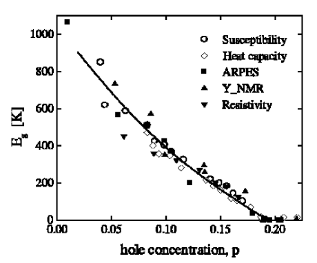
Figure 2: Fig.11 from Tallon et alTallon showing the p-dependence of the pseudogap energy $E_{g}$ or $T^{*}$ determined from susceptibility, heat capacity, ARPES, ⁸⁹Y$\_$NMR and resistivity as displayed in the legends.

Initially, that is above $T_{ps}(p)$, the system has a homogeneous distribution of charge with very small variations around $p$, which is described by a very narrow Gaussian-type distribution. When the temperature goes down through $T_{ps}$ the sample with average hole density $p$ starts to phase separate and the original Gaussian distribution of holes changes continuously into a bimodal type distribution. For underdoped samples with large $T_{ps}$, the mobility $M$ is high which favors a rapid phase separation into two main hole densities $p_{-}$ and $p_{+}$, while the compounds near the critical doping $p_{c}$ may not undergo a complete phase separation. Near the $T_{ps}$, the difference between $p_{-}$ and $p_{+}$ is very small and increases as the temperature goes away from $T_{ps}$. However if the system is quenched very rapidly the phase separation may even not occur, because it depends on the mobility which is essentially the phase separation time scaleBray ; Otton . For $p\geq p_{c}$ there is no phase separation and the charge distribution remains a Gaussian like. For $p\leq p_{c}$, the transformation from a homogeneous phase to one with different densities and with sites at different environment is seemed by many different measurements: by local measurements like, for instance, the Y$\_$NMR, by transport measurements like the resistivity since the charges must overcome the potential barrier $E_{g}$ between the two equilibrium regions (see Fig.(1)) and by susceptibility due to the appearance of antiferromagnetic regions with low hole density specially at the low average doping compounds. Notice that the coefficient $A(T)=\sqrt{(}\alpha(T_{ps}-T))$ changes smoothly as the temperature goes down away from $T_{ps}$ and therefore the charge distribution in a given compound depends strongly on the temperature $T$, on the details of sample synthesis and annealing procedures and, due to the mobility, on how the system is quenched through $T_{ps}$. This is probably the explanation to the different results reported in the literature on many HTSC compounds.

Assuming that the curve proposed by Tallon and LoramTallon reproduced here in the Fig.(2) is the $T_{ps}$ line, the regions below are characterized by their temperature distance from this temperature. The regions in the bottom like 5 to 7, as illustrated in Fig.(3), are region with very strong phase separation while regions near $T_{ps}$ like 1 to 3 the phase separation is weak. This is because $u_{\pm}=\pm(A/B)=\pm\sqrt{(}\alpha(T_{ps}-T)/B)$ and these regions are characterized by their values of $(T_{ps}-T)$. Thus, in region one, the difference between $p_{-}$ and $p_{+}$ is very small and increases as the temperature goes below the $T_{ps}$ line. Accordingly, the energy gap $E_{g}=E_{g}(T)$ is a varying function of $T$ and goes to zero near $T_{ps}$. At zero temperature, compounds with $p\leq 0.1$ may be strongly separated in a insulator phase ($p_{-}\approx 0$) and in a metallic phase with $p_{+}\geq 0.2$. Compounds with $0.1\leq p\leq 0.16$ the phase separation is partial and for $0.16\leq p\leq 0.2$ the original Gaussian is distorted with an increase in the hole density at the low and high tail.

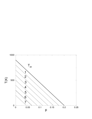
Figure 3: Illustration of the phase separation regions. The thick line represents $T_{ps}$ or $E_{g}$ from Fig.(2) approximated by a straight line. The numbered regions are equidistant from $T_{ps}$ and are characterized by their single values of $(T_{ps}-T)$ which is proportional to the equilibrium densities $p_{-}$ and $p_{+}$.

We have performed calculations in all regions below the phase separation line increasing the value of the $A$ coefficient simulating the the temperature difference $(T_{ps}-T)$. Different initial conditions were tested to check convergence after thousands of time steps. One of the trial starting initial condition was, for instance, $u(t=0)=\varepsilon\times sin(x)sin(y)$.

In Fig.(4) we show the results of the simulations on a $100\times 100$ square grid. In these simulations we used $A/B=0.125$ and $\varepsilon=0.05$ which represents a phase separation in region 4 of Fig.(3) because it is a region where phase separation is neither minimal as in region 1 nor maximal as region 7. The simulation describes the time evolution of a homogeneous initial condition given above and represented by a very sharp Gaussian around the average p value shown in Fig.(5(a)). Fig.(4) shows very clearly the phase separation process.

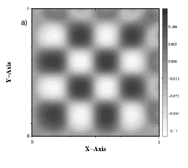
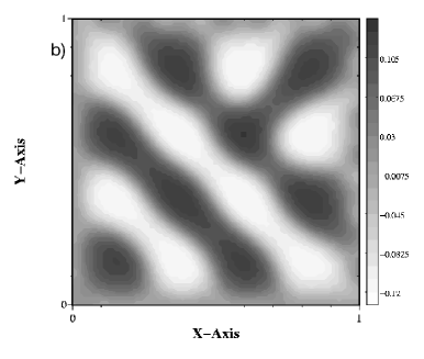
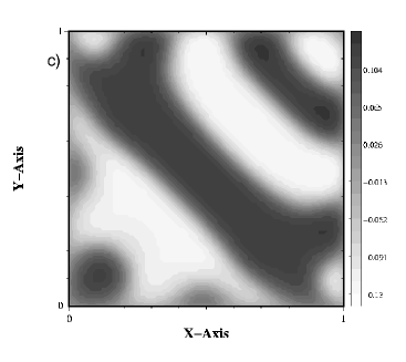
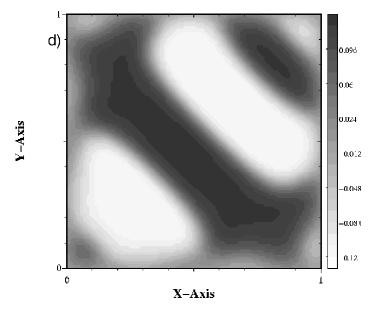
Figure 4: The process of phase separation with the time. On the top panel we plot the order parameter map at the times $t=2000$(a) which displays an (enhanced) reminiscent pattern from the initial conditions, At $t=5000$(b) the phase separation process has already started and on the c) panel at the $t=10000$ and $t=25000$(d).

The phase separation time evolution is also well illustrated by displaying the histogram of how the order parameter evolves in time. In the Fig.(5) we show the time evolution of a typical simulation with the same parameters of Fig.(5): $t=1$ represents the initial condition with the hole density $p(\vec{x})$ centered around an average value $p=0.125$, $t=5000$ represents 5000 time steps in our simulations and so on. It is very interesting the shape of these histogram and their evolution from a initial centered Gaussian to a bimodal distribution. It is very important to emphasize that the distribution after a certain time steps is independent of the initial condition. In practice, if the mobility would be very large and if $\varepsilon$ is very small, the system would evolve to two delta functions at $p_{\pm}$.

Figure 5: The evolution of the local densities of order parameter $u(\vec{x})$ with the time in our simulations. We can see the tendency toward sharps bimodal distributions at the density equilibrium values ($u_{-}$ and $u_{+}$).

To study the effect of the gradient term in the GL free energy of Eq.(1) we have also performed simulations with different values of $\varepsilon$. We have tested $\varepsilon=0.01,0.03$ and $0.05$. The results are shown in Fig.(6) and we can see that indeed the order parameter distribution approaches a delta function as $\varepsilon$ decreases.

Figure 6: The evolution of the local densities of order parameter probability with the gradient constant $\varepsilon$. We can see the tendency toward sharp bimodal formation at the values $p_{\pm}$ as $\varepsilon$ decreases.

Phase separation always occur when we start with a small variation around an average value but the final pattern is strongly dependent on the size of the system. In order to study such effect we have also done, together with the $100\times 100$ lattice, calculation with the $200\times 200$ and $500\times 500$ square grid. At the Fig.(7), we show the results of mapping the order parameter in a surface with the same values of parameter used above. It is very interesting, in the context of HTSC, to observe that smaller lattices display granular pattern and there is a clear increase in the formation of stripes pattern as the size of the lattice is enlarged. It is a matter of fact that the largest HTSC single crystals are those of the $La_{1-x}Sr_{x}Cu0_{2}$ family which are more suitable for neutron diffraction studies and it is exactly in this family which the stripe phases were measuredTranquada ; Bianconi . As conjectured by A.Moreo et alAMoreo , it is likely that the same conclusion may be applied to the manganites.

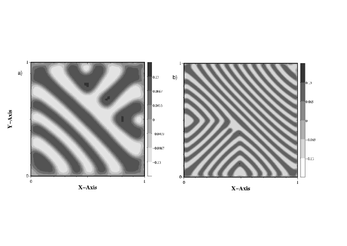
Figure 7: The mapping of the order parameter in the process of phase separation in lattices with different sizes. We display here the order parameter in the $200\times 200$ (a) and for 500$\times$500 (b) lattice. The parameter are the same and therefore it is to be compared with the results displayed in Fig.4d above for the $100\times 100$ lattice.

Notice how the stripe structure develops in the plane interior and as they end at the borders they display a granular type pattern similar to those found in STMXu ; Pan ; Davis . In order the check this we have also performed simulations in 3D. The results does not differ appreciably from the 2D case. At the Fig.(8) we show cuts in a three dimension $100\times 100\times 100$ lattice at the middle plane ($z=50$) and near the top surface ($z=100$).

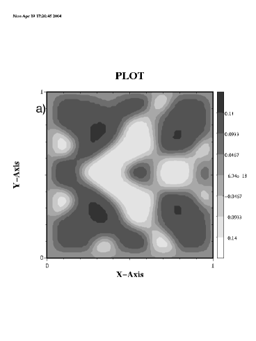
Figure 8: The 3D mapping process of phase separation at t=50000 steps .On the a) panel we plot the order parameter at the center $z=50$ of a $100\times 100\times 100$ lattice. At the b) panel we show the order parameter near the top surface ($z=100$)

IV The Local Gap

We have shown that that below the $T_{ps}$ a phase separation develops creating a variable density of holes at very small mesoscopic scale. Therefore, it is important to perform a local superconducting gap calculation, taking into account this charge inhomogeneity, in order to understand its effect on the the superconductivity phase and specifically, how such phase is built in this inhomogeneous environment. The appropriate way to do this calculation, in a system without spatial invariance, is through the Bogoliubov-deGennes (BdG) mean-field theorySoininen ; Berlinsky ; Franz ; Ghosal ; Ghosal2 . We start with the extended Hubbard Hamiltonian

$$H=-\sum_{\ll ij\gg\sigma}t_{ij}c_{i\sigma}^{\dagger}c_{j\sigma}+\sum_{i\sigma}(V_{i}^{imp}-\mu)n_{i\sigma}+U\sum_{i}n_{i\uparrow}n_{i\downarrow}+{V\over 2}\sum_{\langle ij\rangle\sigma\sigma^{\prime}}n_{i\sigma}n_{j\sigma^{\prime}}$$ (4)

where $c_{i\sigma}^{\dagger}(c_{i\sigma})$ is the usual fermionic creation (annihilation) operators at site ${\bf x}_{i}$, spin $\sigma\{\uparrow\downarrow\}$, and $n_{i\sigma}=c_{i\sigma}^{\dagger}c_{i\sigma}$. $t_{ij}$ is the hopping between site $i$ and $j$, $U$ is the on-site and $V$ is the nearest neighbor interaction. $\mu$ is the chemical potential and $V_{i}^{imp}$ is a random potential which controls the strength of the disorder and introduces the inhomogeneous Hartree shiftGhosal2 .

Using a mean-field decomposition approach, one can define the pairing amplitudesFranz ; Ghosal2 , $\Delta_{\bf\delta}({\bf x}_{i})=V\langle c_{i\downarrow}c_{i+\delta\uparrow}\rangle$ and $\Delta_{U}({\bf x}_{i})=U\langle c_{i\downarrow}c_{i\uparrow}\rangle$, which yields an effective Hamiltonian

$$H_{eff}=-\sum_{i\delta\sigma}t_{i,i+\delta}c_{i\sigma}^{\dagger}c_{i+\delta\sigma}+\sum_{i\sigma}(V_{i}^{imp}-\tilde{\mu}_{i})n_{i\sigma}$$

$$+\sum_{i\delta}[\Delta_{\bf\delta}^{*}({\bf x}_{i})c_{i\downarrow}c_{i+\delta\uparrow}+\Delta_{\bf\delta}({\bf x}_{i})c_{i+\delta\uparrow}^{\dagger}c_{i\downarrow}^{\dagger}]+\sum_{i}[\Delta_{U}({\bf x}_{i})c_{i\uparrow}^{\dagger}c_{i\downarrow}^{\dagger}+\Delta_{U}^{*}({\bf x}_{i})c_{i\downarrow}c_{i\uparrow}].$$ (5)

In this expression ${\bf\delta}$ represents the nearest neighbor vectors and $\tilde{\mu}_{i}=\mu-{U\over 2}\langle n_{i}\rangle$ is the Hartree shift with the local eletronic density $\langle n_{i}\rangle=\sum_{\sigma}\langle n_{i\sigma}\rangle.$ The hole density is $p({\bf x}_{i})=1-\langle n_{i}\rangle$. The $H_{eff}$ is diagonalized by the BdG transformation

$$c_{i\uparrow}= \sum_{n}[\gamma_{n\uparrow}u_{n}({\bf x}_{i})-\gamma_{n\downarrow}^{{\dagger}}v_{n}^{*}({\bf x}_{i})],$$

$$c_{i\downarrow}= \sum_{n}[\gamma_{n\downarrow}u_{n}({\bf x}_{i})+\gamma_{n\uparrow}^{{\dagger}}v_{n}^{*}({\bf x}_{i})]$$ (6)

where $\gamma_{n\sigma}$ and $\gamma_{n\sigma}^{{\dagger}}$ are quasiparticle operators associated with the excitation energies ($E_{n}\geq 0$). $u_{n}({\bf x}_{i})$ and $v_{n}({\bf x}_{i})$ are normalized amplitudes for each ${\bf x}_{i}$. Therefore the BdG equations are

$$\begin{pmatrix}K&\Delta\cr\cr\Delta^{*}&-K^{*}\end{pmatrix}\begin{pmatrix}u_{n}({\bf x_{i}})\cr\cr v_{n}({\bf x_{i}})\end{pmatrix}=E_{n}\begin{pmatrix}u_{n}({\bf x_{i}})\cr\cr v_{n}({\bf x_{i}})\end{pmatrix}$$ (7)

with

$$Ku_{n}({\bf x_{i}}) = -\sum_{\delta}t_{i,i+\delta}u_{n}({\bf x}_{i}+{\delta})+(V_{i}^{imp}-\tilde{\mu}_{i})u_{n}({\bf x}_{i})$$

$$\Delta u_{n}({\bf x_{i}}) = \sum_{\delta}\Delta_{\delta}({\bf x}_{i})u_{n}({\bf x}_{i}+{\delta})+\Delta_{U}({\bf x}_{i})u_{n}({\bf x}_{i}),$$ (8)

and similar equations for $v_{n}({\bf x_{i}})$. These equations give the amplitudes $(u_{n}({\bf x_{i}}),v_{n}({\bf x_{i}}))$, and the eigenergies $E_{n}$. The BdG equations are solved self-consistently together with the pairing amplitudeBerlinsky ; Franz

$$\Delta_{U}({\bf x}_{i}) = -U\sum_{n}u_{n}({\bf x}_{i})v_{n}^{*}({\bf x}_{i})\tanh{E_{n}\over 2k_{B}T},$$ (9)

$$\Delta_{\delta}({\bf x}_{i}) = -{V\over 2}\sum_{n}[u_{n}({\bf x}_{i})v_{n}^{*}({\bf x}_{i}+{\bf\delta})+v_{n}^{*}({\bf x}_{i})u_{n}({\bf x}_{i}+{\bf\delta})]\tanh{E_{n}\over 2k_{B}T},$$ (10)

and the hole density is given by

$$p({\bf x}_{i})=1-2\sum_{n}[|u_{n}({\bf x}_{i})|^{2}f_{n}+|v_{n}({\bf x}_{i})|^{2}(1-f_{n})],$$ (11)

where $f_{n}$ is the Fermi function. Depending on the values of the potentials $V$ and $U$, it is possible to have pairing amplitude with either $s$ or $d$ wave symmetryFranz ; Ghosal ; Ghosal2 .

It has been shownSoininen that a superconducting gap with $d$ wave symmetry calculated in a square lattice, can be written as

$$\Delta_{d}({\bf x}_{i}) = {1\over 4}[\Delta_{\bf\hat{x}}({\bf x}_{i})+\Delta_{-\bf\hat{x}}({\bf x}_{i})-\Delta_{\bf\hat{y}}({\bf x}_{i})-\Delta_{-\bf\hat{y}}({\bf x}_{i})].$$ (12)

Therefore we have used the above BdG theory to calculate the local superconducting zero temperature doping depended $s$ and $d$ wave gap. In Fig.(9), we show a typical set of results for $d$ wave as function of doping, with $V^{imp}=0$ and for a cluster of $14\times 14$ sites. We have used parameters which are appropriated to the HTSC, as we discussed in some of our previous worksEdson01 ; Edson02 : a hopping value of $t=0.35$eV, next neighbor hopping $t_{2}=0.55t$, an on-site repulsion $U=1.3t$ and a next neighbor attraction $V=-1.6$eV. Changing these parameters the gap curve also changes but its qualitative form is not affected. This calculation is to be used concomitantly with the phase separation results from previous sections, since below $T_{ps}$, the system has regions or islands of different doping levels. The consequences of the BdG calculations, like those presented in Fig.(9), will be discussed in the next section in order to support the interpretation of many physical properties associated with the HTSC.

V Discussion

As discussed in the introduction, it is very likely that phase separation is a fundamental process in the HTSC physics and therefore it must manifest itself through many experimental results. In order to explore this fact, we have developed a formalism based on the CH differential equation which allows one to quantitatively study the HTSC phase separation process. We take the upper pseudogap as the onset of phase separation because it starts in the underdoped region usually at very high temperatures ($\approx 800$K) where we expect neither Cooper pair formation nor fluctuation of these pairs and also because there are many arguments against its identification with the superconducting gapTallon . In fact, the difficult to associate the experimental data at such high temperatures with superconductivity led some authors to call it simply a crossover temperatureTS ; Emery . Thus, assuming that the upper pseudogap temperature line as that shown in Fig.(2) is the onset of phase separation, we have been able to provide a simple interpretation to the occurrence of a gap ($E_{g}$) at such high temperatures, to follow the hole density time evolution and how a small fluctuating (almost homogeneous) phase separates into two main local densities ($p_{-}$ and $p_{+}$). Now we want to discuss some more specific implications to the physics of HTSC if, in connection with the above, we take the lower pseudogap as the local onset of superconductivity.

The lower pseudogap has been attributed to the local mean field (MF) superconducting temperature or to the onset of pair formation or superconducting fluctuationEK ; Markiewicz ; Uemura ; Mihailovic . Starting in the underdoped region at temperatures usually near the room temperature, it has been identified with the onset of local superconductivity or with the appearance of small superconducting regionsMello03 . This interpretation is supported by many different experiments, the most directs being the Nernst effectXu ; Wang and muon spin rotationUemura . Following the theoretical predictionsEK and the Nernst effect resultsXu ; Wang , we assume that the lower pseudogap vanishes at the strong overdoped region. Thus, in order to match the lower pseudogap, we have calculated the zero temperature superconducting gap $\Delta(p(\vec{x}))$ with a $d$-wave symmetry as described in the previous section and displayed in Fig.(9). It is important to use small clusters like $8\times 8,12\times 12$ and $14\times 14$ in order to assure that we are indeed calculating the local properties but which are larger than the coherence length.

Figure 9: Results of the calculation for the zero temperature local superconducting gap using a $d$-wave BdG superconducting theory. Since these calculations used a small clusters, we can attribute the average density to a local density $p(\vec{x})$.

It is interesting that the results of the local BdG zero temperature gap function $\Delta(\vec{x})$ have the same qualitative form of the lower pseudogapTS ; EK ; Loram , and it yields large values at low doping with its maximum near $p(\vec{x})\approx 0.05$ and decreases continuously down to zero at the overdoped region. If the $\Delta(p)$ gap measured in a compound with average hole density $p$ is assumed to be the corresponding average value of all $\Delta(p(\vec{x}))$, we arrive that the $\Delta(p(\vec{x}))\times p(\vec{x})$ is very similar to the $\Delta(p)\times p$ curve. Indeed the heat capacity measurements (see Fig.(8) of Tallon and LoramTallon ) and the ARPES (see Fig.(4) of Harris et alHarris ) yield $\Delta(p)\times p$ curves with the same qualitative form of the $\Delta(p(\vec{x}))\times p(\vec{x})$ shown in Fig.(9).

Thus, the lower pseudogap temperature, which we denote $T^{*}(p)$, is the onset of superconductivity and the superconducting regions grow as the temperature is decreased below the $T^{*}(p)$, but long range order is only possible at the percolation limit among these regions, when phase coherence is establish at $T_{c}(p)$. This scenario, with these two (phase-separation and local superconducting) pseudogaps, is appropriate to interpret many non-convention HTSC features and their main phase diagram, that is, the curves $T_{ps}(p)$ (the upper pseudogap temperature), $T^{*}(p)$ (the (superconducting) lower pseudogap temperature) and $T_{c}(p)$, as we discuss below:

We start with the discussion of the many tunneling experiments resultsRenner ; Miyakawa ; Suzuki ; Krasnov00 ; Krasnov ; Yurgens : one of the most well known fact about these experiments is that they do not yield and special signal at $T_{c}(p)$ and form a kind of ”dip” that persists above $T_{c}(p)$ and dies off at $T^{*}(p)$. Our main point is that these experiments are made over a finite region and always measure the average of all $\Delta(p(\vec{x}))$ in this region. As the temperature is continuously raised from near zero, the regions with weaker $\Delta(p(\vec{x}))$ (and lower $T_{c}(p(\vec{x}))$) become initially normal and, increasing more the temperature, many regions gradually turn from superconducting to normal state but, all the local superconducting regions are extinguished only at $T^{*}(p)$, not at $T_{c}(p)$. From the BdG calculations displayed in Fig.(9), we see that the regions with $p$ near $p_{+}$ yield gaps near the minimum value $\Delta(p_{+})$ and we call it the lower or weaker branch. All the $\Delta(p(\vec{x}))$ in this branch which has their local densities $p\leq p(\vec{x})\leq p_{+}$, vanishes before the temperature reaches $T_{c}(p)$ while those in the strong branch $\Delta(p_{-})$ with $p_{-}\leq p(\vec{x})\leq p$ decreases also continuously as temperature is raised but they are more robust and totally vanishes only at $T^{*}$. These features are probed by tunelling experiments which, due to the very small mesoscopic $p(\vec{x})$ regions, usually measure the average of all these gaps. At low temperature, the average of many different gaps are measured and as the temperature is raised they all decrease and, firstly those in the weaker $\Delta(p_{+})$ branch and the ones in the second $\Delta(p_{-})$ afterwards, vanish at different temperatures from zero, passing by $T_{c}(p)$ up to $T^{*}(p)$. Since all different $\Delta(p(\vec{x}))$ vary continuously, there is not any special or different signal at $T_{c}(p)$. The measured $dI/dV$ ”dip” signal which came mostly from the robust gaps in the $\Delta(p_{-})$ branch remains at temperatures well above $T_{c}(p)$ in the underdoped region, decreases for compounds with increasing doping level $p$ since $p_{+}$ and $p_{-}$ approaches one another, and in the overdoped region remains just for a few degrees above $T_{c}(p)$. On the other hand, at the far overdoped region and above the critical doping $p_{c}\approx 0.2$, there is no phase separation and the distribution of $p(\vec{x})$ is just a Gaussian-like distribution around the average hole doping $p$, consequently, the ”dip” structure remains only for a few degrees, proportional to the distribution width. This is well illustrated by Fig.(3) of Suzuki et alSuzuki or in the figures of Renner et alRenner . As mentioned, these experiments see usually the average of many gaps in a given region, but, more recent refined experiments of Krasnov et alKrasnov and Yurgens et al Yurgens were able to distinguish between the gaps in the two average $\Delta(p_{+})$ and $\Delta(p_{-})$ branches. Fig.(1) of Krasnov et alKrasnov shows clearly the weaker $\Delta(p_{+})$ (or superconducting in their interpretation) peak fading away as the temperature approaches $T_{c}(p)$ while the larger average $\Delta(p_{-})$ (or their pseudogap) ”dip” is almost unchanged. They have also shown how applied magnetic fields up to 14T destroy the weaker $\Delta(p_{+})$ leaving again the stronger $\Delta(p_{-})$ branch untouched. Thus, the pseudogap signal remains after the pair coherence is lost because the isolated or local superconducting regions left above $T_{c}$ are those with very large $\Delta(p(\vec{x}))$ or $T_{c}(p(\vec{x}))\leq T^{*}(p)$ and the temperature and fields to destroy the superconductivity in these regions are much larger than $T_{c}(p)$ and the 14T used in the experimentKrasnov . A similar finding was provided by a STM experiment which measured a remaining pseudogap signal inside cores of Bi-2212 quantized vortices, where long range superconductivity is clearly destroyedRenner2 . Furthermore, we predict that the average $\Delta(p_{-})$ maximum peak decreases slowly as the temperature tends to $T_{ps}$ because $p_{+}$ and $p_{-}$ coalesce to $p$. This temperature decreasing was recently measured and can also be seen in Figs. (2 and 3) of Yurgens et al Yurgens .

These results and our interpretation also agrees with the high magnetic field experiments which have measured simultaneously the closing of the pseudogap field ($H_{pg}$) and $T^{*}(p)$ by interlayer tunneling and resistivityLia . Their reported results are for compounds in the overdoped regime with $p\geq p_{c}\approx 0.2$, that is, for compounds with doping level above the phase separation critical doping and $T^{*}(p)$ is just the maximum local $T_{c}(p(\vec{x}))$ or lower pseudogap. At these doping levels there is no phase separation and what Shibauchi et alLia measured as $H_{pg}$ is the field that closes the maximum local critical temperature which is $T^{*}(p)$ because it is the largest of all locals $T_{c}(p(\vec{x}))$. As they apply a magnetic field at low temperature, it destroys first the superconducting clusters with low local $T_{c}(p(\vec{x}))$ and, as the field increases, regions with larger values of the $T_{c}(p(\vec{x}))$ are destroyed. Increasing even more the external field, eventually it destroys the long range order or percolation among the superconducting regions at the superconducting close field $H_{sc}$, leaving still some isolated regions which have larger $T_{c}(p(\vec{x}))$ than the phase coherence temperature $T_{c}(p)$. Increasing more the field, one reaches the closing field $H_{pg}=60$T which destroys all the superconducting regions at $T^{*}(p=0.2)$. The closing field $H_{pg}$ must be very high for compounds with lower doping, probably much higher than the 60T used by Shibauchi et alLia for a $p=0.2$ compound and that is the reason why Krasnov et alKrasnov did not see any change in their optimally doped pseudogap dip at 14T. On the other hand, a d-wave BCS with a Zeeman coupling yields good agreement with the data, supporting the origin of the lower $T^{*}$ as the maximum local superconducting $T_{c}(p(\vec{x}))$Pieri . The fact that the local superconducting regions with large $T_{c}(p(\vec{x}))$ and low local doping (around $p_{-}$) are very robust to an external magnetic field is also consistent with the Knight shift measurements which have seen the reductions of $1/T_{1}T$ and $K$ above $T_{c}$ from the values expected from the normal state at high temperatures in the overdoped region without any field effect up to 23.2T in the underdoped regionZheng . Notice that, since the experiment of Shibauchi et alLia is performed with $p\geq 0.2$ samples, that is above the phase separation threshold $p_{c}$, therefore there is only one (Gaussian) dispersion of local superconducting gaps $\Delta(\vec{x})$ and there is no gap $E_{g}$ associated with any phase separation.

More recently, Hoffman et alHoffman1 ; Hoffman2 and McElroy et alMcElroy ; McElroy2 developed a refined STM analyses which let them to study the doping dependence and the electronic structure of some compounds of the Bi-2212 familyMcElroy2 . They find a distribution of low temperature local superconducting gap values $\Delta(\vec{x})$ whose average value $\Delta(p)$ and its width at half maximum increases for compounds with average hole doping varying between $p\approx 0.19$ and $p\approx 0.11$. The measured local values of $\Delta(\vec{x})$ varies from 20meV to 70meV at regions with linear sides of approximate 55nm in length. The low energy gaps exhibit periodic modulations consistent with charge modulations like of a granular charge phase separation. Their results, specially those shown in their Fig.(3A-3E), display a distribution of mesoscopic scale regions local gaps of two types:
a) One type derived from a $dI/dV$ curve with sharp edges with values $<65$meV which they called coherence peaks. They interpreted this type of peaks as due to superconducting pairing on the whole Fermi Surface arguing that this kind of spectrum is consistent with a d-wave superconducting gapHoffman2 .
b) Another type of $dI/dV$ spectra display an ill defined edges of a V-shape gap with larger values than +65meV what they called zero temperature pseudogap spectrum. Furthermore, they find that the a-type spectra are dominant for overdoped samples ($p=0.19$ and $0.18$) in which there is practically $0\%$ probability of occurring spectra of b-type. The b-type spectra start to have a nonzero probability for compounds with $p=0.14$ or below, and for underdoped compounds like $p=0.11$ they find more than $55\%$ of b-type spectra. It is not difficult to explain these observations in terms of the CH phase separation scenario: The $p=0.19$ and $0.18$ compounds are near the phase separation threshold and their $p(\vec{x})$ distribution is essentially a Gaussian type, $E_{g}$ is small and they measure a Gaussian distribution of local superconducting gap values $\Delta(\vec{x})$ or a-type spectra. On the other limit, for the $p=0.11$ compound, according to the phase separation histogram of Fig.(5), almost half of the system has very low doping ($0<p(\vec{x})<0.5$), the $p_{-}$ branch and almost half of the system is in the other $p_{+}$ branch ($0.17<p(\vec{x})<0.22$). The regions with $p(\vec{x})$ in the $p_{+}$ branch exhibit a superconducting gap distribution of a-type spectra, while regions in the $p_{-}$ branch are mainly in the insulating region which produces b-type spectra. These a- and b-type spectra are mixed in the intermediated $p=0.15$ and $p=0.13$ compounds and it is in this near optimal doping region that both superconducting and the b-type gap have equally probability. Consequently, the gap maps found by Hoffman et alHoffman1 ; Hoffman2 and McElroy et alMcElroy ; McElroy2 are a clear manifestation of the phase separation process in Bi2212.

There are many other experiments which we could discuss in the light of the present phase separation theory but we believe that the above discussion is sufficient to demonstrate that phase separation process is central to understand many non-conventional HTSC properties.

VI Conclusions

We have studied analytically the problem of phase separation in HTSC taking some current ideas on the possibility to identify the upper $T^{*}$ with the onset of phase separation and the lower pseudogap as the onset of d-wave superconductivity. Our approach allows us to make quantitative calculations of the phases separation process and to perform simulations which led to granular and stripe patterns depending on the parameter and size of the lattice, which are in agreement with current observations. Such calculations might be also be pertinent to the physics of manganites. It is also possible to get some insights on many general experimental results like:
i-The charge distribution becomes more inhomogeneous in the underdoped region of the phase diagram where the stripes has been observed because $T_{ps}$ is larger in this region.
ii-The spatial variation or width of the local hole concentration $p(\vec{x})$ increases as the temperature decreases.
iii-The fact that some materials exhibit granular while others exhibit stripe patterns may be related with the single crystal or palette size of ceramic or granular samples. Our simulations indicate that larger lattices favor stripe patterns while smaller ones favor granular patterns.
iv-The spinodal decomposition reveals the importance of the sample preparation process, that is, samples with the same doping level may have different degree of inhomogeneity depending on the way they have been quenched through $T_{ps}$. This would explain different results on the same kind of compounds which has been very frequent in the HTSC.
v-The two different signal detected by refined tunelling experiments.
vi-The density os state modulation measured by recent STM data.

In summary, the CH phase separation approach to HTSC in connection with local charge density dependent BdG superconducting critical temperature calculation is used to explain the existence and nature of the two different pseudogaps and it provides novel interpretations on many non-conventional features and inhomogeneous patterns. Therefore, our main point is that we should regard the phase separation process as one of the key ingredients of the HTSC physics.

VII Acknowledgment

We gratefully acknowledge partial financial aid from Brazilian agencies CNPq and FAPERJ.

References

- (1) T. Timusk and B. Statt, Rep. Prog. Phys., 62, 61 (1999).
- (2) J.L. Tallon and J.W. Loram, Physica C 349, 53 (2001).
- (3) H. Alloul, T. Ohno, P. Mendels, Phys. Rev. Lett.63, 1700 (1989).
- (4) V.J. Emery, S.A. Kivelson, and O. Zachar, Phys. Rev. B56 6120 (1997).
- (5) D. Mihailovic, V. V. Kabanov, K. Zagar, and J. Demsar, Phys. Rev. B60. R6995 (1999).
- (6) V.J. Emery, and S.A. Kivelson, Nature 374, 434 (1995).
- (7) J. Corson et al, Nature 398, 221 (1999).
- (8) C. Bernhard, D. Munzar, A. Golnik, C. T. Lin, A. Wittlin, J. Humlicek, and M. Cardona, Phys. Rev. B61, 618 (2000).
- (9) Z.A. Xu, N.P. Ong, Y. Wang, T. Kakeshita, and S. Uchida, Nature 406, 486 (2000) and cond-mat/0108242.
- (10) Yayu Wang, N. P. Ong, Z. A. Xu, T. Kakeshita, S. Uchida, D. A. Bonn, R. Liang, and W. N. Hardy Phys. Rev. Lett.88, 257003 (2002).
- (11) C. Meingast, V. Pasler, P. Nagel, A. Rykov, S. Tajima, and P. Olsson, Phys. Rev. Lett.86, 1606 (2001).
- (12) R.S. Markiewicz, Phys. Rev. Lett.89, 229703 (2002).
- (13) A. Ino, C. Kim, M. Nakamura, T. Yoshida, T. Mizokawa, A. Fujimori, Z.-X. Shen, T. Kakeshita, H. Eisaki, and S. Uchida, Phys. Rev. B 65, 094504 (2002).
- (14) Ch. Renner, B. Revaz, J.Y. Genoud, K. Kadowaki, O. Fischer, Phys. Rev. Lett.80, 149 (1998).
- (15) N. Miyakawa, P. Guptasarma, J. F. Zasadzinski, D. G. Hinks, and K. E. Gray , Phys. Rev. Lett.80, 157 (1998).
- (16) Minoru Suzuki, and Takao Watanabe, Phys. Rev. Lett.85 4787, (2000).
- (17) J.M. Harris, Z. -X. Shen, P. J. White, D. S. Marshall, and M. C. Schabel, J. N. Eckstein and I. Bozovic, Phys. Rev. B54, R15665 (1996).
- (18) M. Kugler, O. Fischer, Ch. Renner , S. Ono and Yoichi Ando, Phys. Rev. Lett.86, 4911 (2001).
- (19) Y.J. Uemura, Sol. St. Comm. 126, 23 (2003).
- (20) P. Pieri, G.C. Strinati, and D. Moroni, Phys. Rev. Lett 89, 127003 (2002).
- (21) V.M. Krasnov, A. Yurgens, D. Winkler, P. Delsing, and T. Claeson, Rev. Lett.84, 5860 (2000).
- (22) V.M. Krasnov, A. E. Kovalev, A. Yurgens, and D. Winkler Phys. Rev. Lett. 86 2657 (2001).
- (23) A. Yurgens, D. Winkler, T. Claeson, S. Ono, and Yoichi Ando, Phys. Rev. Lett. 90, 147005 (2003).
- (24) See Phase Separation in Cuprates Superconductors, edited by E. Sigmund and K.A. Müller (Spring-Verlag, Berlin, 1994).
- (25) A.H. Castro Neto, Phys. Rev. B51, 3254 (1995).
- (26) B.W. Statt, P. C. Hammel, Z. Fisk, S-W. Cheong, F. C. Chou, D. C. Johnston, and J. E. Schirber, Phys. Rev. B52, 15575 (1995).
- (27) E.W. Carlson et al, in ”The Physics of Conventional and Unconventional Superconductors” ed. by K. H. Bennemann and J. B. Ketterson (Springer-Verlag) (2003) and cond-mat/0206217.
- (28) J. Wang, D. Y. Xing, Jinming Dong, and P.H. Hor, Phys. Rev. B62, 9827 (2000).
- (29) J. Zaanen, and O. Gunnarsson, Phys. Rev. B40, 7391 (1989).
- (30) J.M.Tranquada, B.J. Sternlieb, J.D. Axe, Y. Nakamura, and S. Uchida, Nature (London),375, 561 (1995).
- (31) A. Bianconi, N.L. Saini, A. Lanzara, M. Missori, T. Rossetti, H. Oyanagi, H. Yamaguchi, K. Oka and T. Ito, Phys. Rev. Lett. 76, 3412 (1996).
- (32) S. H. Pan et al, Nature, 413, 282-285 (2001) and cond-mat/0107347.
- (33) K.M. Lang et al, Nature, 415, 412 (2002).
- (34) J.W. Loram, J.L. Tallon and W.Y. Liang, Phys. Rev. B69, R060502 (2004).
- (35) E.S. Bozin, G.H. Kwei, H. Takagi, and S.J.L. Billinge, Phys. Rev. Lett. 84, 5856, (2000).
- (36) P.M. Singer, A.W. Hunt, and T. Imai, Phys. Rev. Lett. 88, 047602, (2002).
- (37) A. Moreo, S. Younoki, and E. Dagotto, Science, 283, 2034 (1999).
- (38) E. Dagotto, T. Hotta and, A. Moreo, Phys. Rep. 344, 1 (2001).
- (39) E. Dagotto, J. Burgy, A. Moreo, Sol. St. Comm. 126, 9, (2003).
- (40) B. Lorenz, Y. Y. Xue, and C. W. Chu, in ”Studies of High-Temperature Superconductors”, Vol. 46, ed. A. V. Narlikar (Nova Science Publ., New York, 2003)
- (41) A.J. Bray, Adv. Phys. 43, 347 (1994).
- (42) J.W. Cahn and J.E. Hilliard, J. Chem. Phys, 28, 258 (1958).
-
(43)
D.J. Eyre,
http://www.math.utah.edu/ eyre/research/
methods/stable.ps) (1998). - (44) E.V.L de Mello, and Otton T. Silveira Filho submitted to Comp. Phys. Com. (2004).
- (45) I. Iguchi, I. Yamaguchi, and A. Sugimoto, Nature, 412, 420 (2001).
- (46) A. Lascialfari, A. Rigamonti, L. Romano, P. Tedesco, A. Varlamov, and D. Embriaco, Phys. Rev. B65, 144523 (2002).
- (47) A. Lascialfari, A. Rigamonti, L. Romano, A.A. Varlamov, and I. Zucca, Phys. Rev. B68 100505(R), (2003).
- (48) J.L. González, and E.V.L. de Mello. Phys. Rev. B69, 134510 (2004).
- (49) Yu.N. Ovchinnikov, S.A. Wolf, V.Z. Kresin, Phys. Rev. B63, 064524, (2001), and Physica C341-348, 103, (2000).
- (50) D. Mihailovic, V.V. Kabanov, K.A. Müller, Europhys. Lett. 57, 254 (2002).
- (51) E.V.L. de Mello, E.S. Caixeiro, and J.L. González, Phys. Rev. B67, 024502 (2003).
- (52) E.S. Caixeiro, J.L. González, and E.V.L. de Mello. Phys. Rev. B69, 024521 (2004).
- (53) P.I. Soininen, C. Kallin, and A.J. Berlinsky, Phys. Rev. B 50, 13883 (1994).
- (54) M. Franz, C. Kallin, and A.J. Berlinsky, Phys. Rev. B54, R6897 (1996).
- (55) M. Franz, C. Kallin, A.J. Berlinsky, and M.I. Salkola, Phys. Rev. B 56, 7882 (1997).
- (56) A. Ghosal, M. Randeria, and N. Trivedi, Phys. Rev. B63, R020505 (2000).
- (57) A. Ghosal, M. Randeria, and N. Trivedi, Phys. Rev. B 65, 014501 (2001).
- (58) E.S. Caixeiro, E.V.L. de Mello, Physica C 353, 103 (2001).
- (59) E.S. Caixeiro, E.V.L. de Mello, Physica C 383, 89 (2002).
- (60) Ch. Renner, B. Revaz, K. Kadowaki, I. Maggio-Aprile, O. Fischer, Phys. Rev. Lett.80, 3606 (1998).
- (61) T. Shibauchi, L. Krusin-Elbaum, Ming Li, M.P. Maley, and P.H. Kes, Phys. Rev. Lett 86, 5763 (2001).
- (62) Guo-qing Zheng, H. Ozaki, W. G. Clark, Y. Kitaoka, P. Kuhns, A. P. Reyes, W. G. Moulton, T. Kondo, Y. Shimakawa, and Y. Kubo Phys. Rev. Lett. 85, 405 (2000).
- (63) J. E. Hoffman, E. W. Hudson, K. M. Lang, V. Madhavan, H. Eisaki, S. Uchida, J.C. Davis, Science 295, 466 (2002)
- (64) J. E. Hoffman, K. McElroy, D.-H. Lee, K. M Lang, H. Eisaki, S. Uchida, J.C. Davis, Science 297, 1148-1151 (2002).
- (65) K. McElroy, R.W Simmonds, J. E. Hoffman, D.-H. Lee, J. Orenstein, H. Eisaki, S. Uchida, J.C. Davis, Nature, 422, 520 (2003).
- (66) K. McElroy, D.-H. Lee, J. E. Hoffman, K. M Lang, E. W. Hudson, H. Eisaki, S. Uchida, J. Lee, J.C. Davis, cond-mat/0404005.