Driven Diffusive Systems: How Steady States Depend on Dynamics

Abstract

In contrast to equilibrium systems, non-equilibrium steady states depend explicitly on the underlying dynamics. Using Monte Carlo simulations with Metropolis, Glauber and heat bath rates, we illustrate this expectation for an Ising lattice gas, driven far from equilibrium by an ‘electric’ field. While heat bath and Glauber rates generate essentially identical data for structure factors and two-point correlations, Metropolis rates give noticeably weaker correlations, as if the ‘effective’ temperature were higher in the latter case. We also measure energy histograms and define a simple ratio which is exactly known and closely related to the Boltzmann factor for the equilibrium case. For the driven system, the ratio probes a thermodynamic derivative which is found to be dependent on dynamics.

I Introduction

In statistical physics, Monte Carlo (MC) simulations play a major role for the study of phase transitions and critical phenomena, as well as ordered and disordered phases MC . Leaving out many details of the art of computing, the broad outline of the simulation process is easily summarized. For systems both in and far from thermal equilibrium, dynamic rates $W[\sigma\rightarrow\sigma^{\prime}]$ are defined which specify how a given configuration $\sigma$ evolves into a new one, $\sigma^{\prime}$, when an update is attempted. The simulations then generate long sequences of such configurations. Once initial transients have decayed, time-independent (stationary) observables – which will be our focus in the following – can be computed as configurational averages. For a system in thermal equilibrium, characterized by a Hamiltonian $\mathcal{H}$, it is well known that any choice of $W$’s, as long as they satisfy detailed balance with respect to $H$, will generate configurations distributed according to the same Boltzmann factor, $\exp(-\beta H)$. In other words, time-independent observables, including both universal and non-universal properties, are independent of the choice of rates, provided detailed balance holds. The resulting freedom can be exploited to design particularly efficient codes, such as cluster algorithms SW . In stark contrast, no such ‘decoupling’ of dynamic and stationary characteristics occurs for systems driven out of equilibrium: even though non-equilibrium steady states (NESS) display time-independent observables, these are sensitive to modifications of the dynamic rates. This behavior can be traced back to the violation of detailed balance which is an inherent feature of non-equilibrium systems SZ ; revs .

While the sensitivity of NESS to the choice of the dynamics has been noted before KLS ; Krug , no systematic computational study has yet been undertaken. In this paper, we consider two models: the standard Ising lattice gas and its non-equilibrium cousin, the driven Ising lattice gas (or KLS model, after the initials of its inventors KLS ). Both involve particles diffusing on a lattice, subject to an excluded volume constraint and an (attractive) nearest-neighbor interaction. The total number of particles remains conserved. For the Ising lattice gas, the rates for particle hops to unoccupied nearest-neighbor sites are chosen to satisfy detailed balance, with respect to the Ising Hamiltonian. In contrast, the driven version involves an additional external force which acts on the particles much like an electric field on (positive) charges: aligned with a lattice axis (e.g., $y$), it favors particle hops along its direction. In conjunction with periodic boundary conditions, this bias breaks detailed balance and establishes a non-equilibrium steady state. This NESS differs drastically from its equilibrium counterpart, exhibiting generic long-range correlations, a novel universality class, and highly anisotropic ordered phases SZ .

To illustrate the importance of the transition rates for the NESS, we measure structure factors and two-point spatial correlations in the driven case, using Metropolis Met , Glauber glauber , and heat bath heatbath rates. To date, simulations of the driven model have focused almost exclusively on Metropolis rates VM ; other rates have only been invoked in some analytic studies Krug ; ana . While the first two are easily implemented for conserved particle number, an appropriate generalization of heat bath rates is designed here for the first time. To avoid complications due to inhomogeneous ordered phases, we choose temperatures above or at criticality. For comparison, we also show the same quantities for the (equilibrium) Ising model: as expected, they are found to be identical up to statistical fluctuations, and almost perfectly isotropic. In stark contrast, when the drive is turned on, we find strongly anisotropic behavior and markedly different values for the three choices of rates. While all driven cases exhibit the signatures of long-ranged decay in real space, the correlations are much weaker for Metropolis rates than for either Glauber or heat bath ones.

As an additional probe into the differences between the standard Ising lattice gas and its driven cousin, we construct energy histograms (with respect to the Ising Hamiltonian) for both. For the equilibrium case, these are of course intimately related to the Boltzmann distribution and contain a wealth of thermodynamic information. For the driven system, they are easily measured in a simulation, but their physical interpretation has not been established yet. Here, we consider a simple histogram ratio whose equilibrium limit is easily derived, and compute its non-equilibrium counterpart.

This paper is organized as follows. We first introduce our models and the three types of dynamics, followed by a brief discussion of our key observables. We then present our data for two-point correlations, structure factors and energy histograms. We conclude with a summary, offering a conjecture for the origin of the observed differences between the three rate functions.

II Background

II.1 The models

In this section, we introduce our two prototype models, namely, the Ising lattice gas and its driven version. Both are defined on an $M\times L$ square lattice in two dimensions, with fully periodic boundary conditions. Each site $\mathbf{i}$ is either occupied by a particle or empty, which we denote by a spin variable $\mathbf{\sigma_{i}}$ taking two values: $+1$ (occupied) or $-1$ (empty). For the equilibrium Ising model, we can specify a (global) Hamiltonian:

$$\mathcal{H}[\sigma]=-J\sum_{<\mathbf{i},\mathbf{j}>}\mathbf{\sigma_{i}\,\sigma_{j}},$$ (1)

where the sum runs over nearest-neighbor pairs of sites, and $J>0$ denotes the binding energy. In order to access the Ising critical point, we consider only half-filled systems: $(LM)^{-1}\sum_{\mathbf{i}}\sigma\mathbf{{}_{i}}=0$. When coupled to a heat bath at temperature $T$, the probability, $P_{0}(\sigma)$, to find the system in configuration $\sigma$ is controlled by the well-known Boltzmann factor: $P_{0}(\sigma)\propto\exp(-\beta H)$ with $\beta=1/k_{B}T$. Here and in the following, the subscript $0$ will always denote equilibrium quantities.

The usual technique for simulating such a distribution is to introduce a dynamics in configuration space. We choose a suitable set of transition rates, $W[\sigma\rightarrow\sigma^{\prime}]$, which specify how a configuration $\sigma$ evolves into a new one, $\sigma^{\prime}$, in unit time. For simplicity, we only consider transitions in which $\sigma$ and $\sigma^{\prime}$ differ by a single nearest-neighbor particle-hole exchange. Now, the probability distribution, $P(\sigma,t)$, becomes time-dependent and satisfies a master equation (written, for simplicity, in continuous time):

$$\partial_{t}P(\sigma,t)=\sum_{\sigma^{\prime}}\left\{W[\sigma^{\prime}\rightarrow\sigma]P(\sigma^{\prime},t)-W[\sigma\rightarrow\sigma^{\prime}]P(\sigma,t)\right\}$$ (2)

Its stationary solution, $P(\sigma)\equiv\lim_{t\rightarrow\infty}P(\sigma,t)$, controls all time-independent properties. It is unique, under fairly generic conditions on the rates. To ensure that the desired equilibrium distribution, $P_{0}(\sigma)$, is reproduced, one chooses $W$’s which satisfy the detailed balance condition:

$$\frac{W[\sigma\rightarrow\sigma^{\prime}]}{W[\sigma^{\prime}\rightarrow\sigma]}=\frac{P_{0}(\sigma^{\prime})}{P_{0}(\sigma)}=e^{-\beta\left\{\mathcal{H}[\sigma^{\prime}]\mathcal{-H}[\sigma]\right\}}$$ (3)

Of course, this just ensures that every $\left\{...\right\}$ bracket in Eq. (2) vanishes. An important quantity which enters here is the energy difference of two configurations, $\sigma^{\prime}$ and $\sigma$:

$$\Delta_{0}\equiv\mathcal{H}[\sigma^{\prime}]\mathcal{-H}[\sigma]$$ (4)

A simple way of satisfying detailed balance is to impose rates which are functions of this difference alone: $W[\sigma\rightarrow\sigma^{\prime}]\equiv w(\beta\Delta_{0})$ where the function $w$ must satisfy

$$w(x)=w(-x)e^{-x}\quad,$$ (5)

by virtue of Eq. (3) but is otherwise arbitrary. All three rate functions to be considered below – Metropolis, Glauber, and heat bath – are constructed in this way, but differ in some important details.

An obvious way of driving a system into a non-equilibrium steady state is to impose rates that violate detailed balance. A prototype model that has attracted much interest due to its remarkable properties is the driven Ising lattice gas (or KLS model) KLS ; SZ . It differs from the standard Ising model through the presence of an external force $\mathcal{E}$, aligned with a particular lattice axis (the $y$-direction). When a particle attempts to jump to an empty nearest-neighbor site, it is not only affected by the local energetics, incorporated in Eq. (1), but also by the drive: similar to an electric field, $\mathcal{E}$ favors (suppresses) particle hops along (against) the selected direction, leaving transverse exchanges unaffected. A straightforward extension of Eq. (4) is to include the work done by the field, i.e., to define a local ‘energy’ difference of the form

$$\Delta\equiv\mathcal{H}[\sigma^{\prime}]\mathcal{-H}[\sigma]-\epsilon\mathcal{E}$$ (6)

Here, $\epsilon=0$ for two configurations differing only by a transverse jump, and $\epsilon=+1$ $(-1)$ if the particle hops along (against) the field in the move. We can now choose rates of the form (5) with $x=\beta\Delta$. However, it is essential to note that the combination of uniform drive and periodic boundary conditions precludes the existence of a global Hamiltonian for the driven system. A unique steady state, $P(\sigma)$, establishes itself but cannot be expressed in terms of a Boltzmann factor. To maximize the non-equilibrium effects, we choose infinite $\mathcal{E}$ for our simulations, i.e., a particle will never jump against the field.

II.2 Three different rate functions.

In this subsection, we introduce the three choices of transition rates – Metropolis, Glauber, and heat bath – which will be compared in the following. For the first two choices, the relevant quantity is the local ‘energy’ difference between the final ($\sigma^{\prime}$) and the initial ($\sigma$) configuration. For the third choice, the rate is independent of the initial configuration; instead, the selection criterion involves the local energy difference of the two possible final configurations, $\sigma$ and $\sigma^{\prime}$. For the equilibrium Ising model, energy differences are easily computed from Eq. (4), and each rate satisfies the detailed balance condition; for the driven model, we invoke Eq. (6), and detailed balance is violated. Random numbers are selected uniformly from the interval $(0,1)$.

Metropolis dynamics. For this choice of rates, we randomly select a nearest-neighbor pair $\mathbf{i}$, $\mathbf{j}$ of sites with different occupanices, $\sigma_{\mathbf{i}}\neq\sigma_{\mathbf{j}}$. We denote the original configuration as $\sigma$ and let $\sigma^{\prime}$ be the configuration with $\sigma_{\mathbf{i}}$, $\sigma_{\mathbf{j}}$ switched (i.e., $\sigma_{\mathbf{i}}^{\prime}=\sigma_{\mathbf{j}}$; $\sigma_{\mathbf{j}}^{\prime}=\sigma_{\mathbf{i}}$). The transition from $\sigma$ to $\sigma^{\prime}$ is controlled by the Metropolis rate function, $w_{Met}(x)=\min(1,e^{-x})$. To be specific, we first compute $x=\beta\Delta$. If $x\leq 0$, the attempt (exchange) is accepted; if, however, $x>0$, we draw a random number $z$ and perform the exchange only if $z\leq e^{-x}$. Clearly, energetically favorable moves are always performed while only a fraction of costly ones is accepted. As temperature increases, this fraction approaches $1$ in a monotonic fashion.

Glauber dynamics. Similar to Metropolis dynamics, the implementation of this algorithm involves, first, selecting two nearest-neighbor sites with different occupancies. Again, $\sigma^{\prime}$ refers to the configuration with switched occupancies. Exchanges are then controlled by the Glauber rate function, $w_{Gl}(x)=1/(1+e^{x})$. Again, we compute $x=\beta\Delta$ and draw a random number, $z$. If $z\leq 1/(1+e^{x})$, we accept the exchange; otherwise, it is rejected. While energetically favorable moves are not necessarily accepted, they are always more probable than unfavorable ones.

Heat bath dynamics. As pointed out above, the interpretation of $\sigma$ and $\sigma^{\prime}$ is different here: These refer to the two possible final configurations of the central particle-hole pair. Showing only its local neighborhood in the lattice, we define

σ2−1+1σ5σ1σ6𝜎

σ3σ4

	σ3	σ4
σ2	+1	−1	σ5
	σ1	σ6

 and superscript𝜎′fragments σ3 σ4 fragmentsσ2fragments1fragments1fragmentsσ5missing-subexpressionfragmentsσ1fragmentsσ6missing-subexpression\sigma\equiv\begin{tabular}[]{|l|l|l|l|}\hline\cr&$\sigma_{3}$&$\sigma_{4}$&\\ \hline\cr$\sigma_{2}$&$+1$&$-1$&$\sigma_{5}$\\ \hline\cr&$\sigma_{1}$&$\sigma_{6}$&\\ \hline\cr\end{tabular}\text{ and }\sigma^{\prime}\equiv\begin{tabular}[]{|l|l|l|l|}\hline\cr&$\sigma_{3}$&$\sigma_{4}$&\\ \hline\cr$\sigma_{2}$&$-1$&$+1$&$\sigma_{5}$\\ \hline\cr&$\sigma_{1}$&$\sigma_{6}$&\\ \hline\cr\end{tabular} (7)

for bonds along the $x$-axis, and

σ1−1σ3σ6+1σ4σ5𝜎

σ2

	σ2
σ1	+1	σ3
σ6	−1	σ4
	σ5

 and superscript𝜎′fragments σ2 fragmentsσ1fragments1fragmentsσ3fragmentsσ6fragments1fragmentsσ4missing-subexpressionfragmentsσ5missing-subexpression\sigma\equiv\begin{tabular}[]{|l|l|l|}\hline\cr&$\sigma_{2}$&\\ \hline\cr$\sigma_{1}$&$+1$&$\sigma_{3}$\\ \hline\cr$\sigma_{6}$&$-1$&$\sigma_{4}$\\ \hline\cr&$\sigma_{5}$&\\ \hline\cr\end{tabular}\text{ and }\sigma^{\prime}\equiv\begin{tabular}[]{|l|l|l|}\hline\cr&$\sigma_{2}$&\\ \hline\cr$\sigma_{1}$&$-1$&$\sigma_{3}$\\ \hline\cr$\sigma_{6}$&$+1$&$\sigma_{4}$\\ \hline\cr&$\sigma_{5}$&\\ \hline\cr\end{tabular} (8)

for bonds along $y$; i.e., parallel to the drive. We also define

$$h\equiv\sum_{\mathbf{i}=1}^{3}\sigma_{\mathbf{i}}-\sum_{\mathbf{i}=4}^{6}\sigma_{\mathbf{i}}$$ (9)

In equilibrium, the heat bath algorithm is of course isotropic: For both types of bonds, we select configuration $\sigma$ if a random number $z$ satisfies $z\leq 1/(1+e^{-2\beta h})$; otherwise, we choose $\sigma^{\prime}$. For the driven case, this rule is only applied to bonds transverse to the drive; for parallel bonds, at infinite $\mathcal{E}$, we choose configuration $\sigma$ with probability $1$.

Figure 1: A central pair and a particular configuration of its six nearest neighbors. Occupied sites are indicated by solid circles.

To appreciate the commonalities and differences of the three algorithms, it is useful to consider a simple example with infinite drive. Fig. 1 shows a central pair and a particular configuration of its six nearest neighbors. If the pair is aligned with the field direction (Figs. 1a, b), all three dynamics generate the same outcome: each will select Fig. 1a as the final configuration with probability $1$ for any value of $\beta J$.

This is not the case for bonds transverse to the field (Figs. 1c, d). For the purposes of this argument, we choose $\beta J=0.1$. We denote the configuration shown in Fig. 1c (d) by $\sigma$ ($\sigma^{\prime}$). The ‘energy’ difference $\Delta=12J$ is easily computed from Eq. (4) or (6). Given a random number $z$, the Metropolis algorithm will accept a transition from $\sigma$ to $\sigma^{\prime}$ only if $z\leq$ $e^{-12\beta J}\simeq 0.30$, while the reverse transition ($\sigma^{\prime}$ to $\sigma$) is always accepted. For Glauber dynamics, the transition from $\sigma$ to $\sigma^{\prime}$ is accepted if $z$ $\leq 1/(1+e^{12\beta J})$ $\simeq$ $0.23$, while the reverse transition is accepted if $z$ $\leq 1/(1+e^{-12\beta J})\simeq 0.77$. Finally, the heat bath algorithm will choose $\sigma$ as the final state if $z$ $\leq 1/(1+e^{-12\beta J})\simeq$ $0.77$, and $\sigma^{\prime}$ otherwise.

The notable differences are these: First, the Metropolis algorithm accepts unfavorable moves with higher probability than either heat bath or Glauber: $e^{-x}\geq$ $1/(1+e^{x})$. As a result, it is more likely to explore unphysical domains of configuration space. Yet, it also accepts favorable moves with higher probability, and thus leads to a more active dynamics. Comparing heat bath and Glauber rates, we note that both subdivide the unit interval into the same subsections ($0.23$ vs $0.77$). Hence, they generate statistically very similar trajectories in configuration space. Update by update, however, the trajectories can differ: if, e.g., the initial configuration is $\sigma$ and the random number turns out to be $0.1$, the heat bath algorithm will choose $\sigma^{\prime}$ as the final configuration, while the Glauber rule leads to an exchange since $z<0.23$. Yet, we will see below that this subtle difference does not affect the data.

II.3 Structure factors and two-point correlations.

Below their critical temperatures, both the Ising lattice gas and the KLS model phase-segregate into regions of high and low density, by virtue of the conservation law on the number of particles. Typical low-temperature configurations, for both models, show a single strip of high-density phase and its low-density mirror image. For the Ising model, the strip orients itself such as to minimize the energetic cost of interfacial length. In contrast, the low-temperature strip of the KLS model is always aligned with the direction of the drive, and the minimization of interfacial length does not play a dominant role (cf. Fig. 2). A quantity which easily distinguishes disordered configurations from such inhomogeneous ones is the (equal-time) structure factor. Written in spin language, it is defined as

$$S(\mathbf{k})=\frac{1}{ML}\left\langle\left|\sum_{\mathbf{j}}e^{i\mathbf{k}\cdot\mathbf{j}}\sigma_{\mathbf{j}}\right|^{2}\right\rangle.$$ (10)

Here, $\mathbf{k}$ is a wave vector, taking discrete values $\mathbf{k}=(2\pi n_{x}/M,2\pi n_{y}/L)$ with $n_{x}=0,1,...,M-1$ and $n_{y}=0,1,...,L-1$. For simplicity, we write $S(n_{x},n_{y})$ in the following, and use $S(1,0)$ and $S(0,1)$ to detect strips aligned with the $y$- or $x$-axis, respectively. For a perfectly ordered strip aligned with $y$, $S(1,0)\simeq 0.41ML$ is maximized; in contrast, a disordered configuration results in $S(1,0)=O(1)$. Further, the structure factor is the Fourier transform of the two-point correlation function, $G(\mathbf{r})$, defined via

$$G\left(\mathbf{r}\right)\equiv\left\langle\sigma_{\mathbf{0}}\sigma_{\mathbf{r}}\right\rangle-\left\langle\sigma_{\mathbf{0}}\right\rangle\left\langle\sigma_{\mathbf{r}}\right\rangle$$ (11)

We assume translational invariance (modulo the lattice size) and invoke the half-filling constraint, whence $\left\langle\sigma_{\mathbf{r}}\right\rangle=\left\langle\sigma_{\mathbf{0}}\right\rangle=0$. The same constraint imposes the sum rule $\sum_{\mathbf{r}}G\left(\mathbf{r}\right)=S(\mathbf{0})=0$. Hence, negative values of $G\left(\mathbf{r}\right)$ for certain values of the argument should not come as a surprise.

II.4 Energy histograms.

For both the equilibrium Ising model and its driven counterpart, it is straightforward to accumulate a (normalized) energy histogram $H(E,\beta)$, with respect to the energy function defined in Eq. (1). For the equilibrium Ising model, $H_{0}(E,\beta)$ is intimately related to the Boltzmann distribution: if $W\left(E\right)$ denotes the density of states and $Z(\beta)$ the canonical partition function, we have

$$H_{0}\left(E,\beta\right)=Z^{-1}(\beta)W\left(E\right)e^{-\beta E}$$ (12)

Clearly, the right hand side is the probability $P_{0}(E,\beta)$ to find the system with energy $E$. The power of the histogram method hist resides in the observation that, up to statistical errors, a single histogram measured at temperature $1/\beta$ is sufficient to construct $P_{0}(E,\beta^{\prime})$ at all other temperatures $1/\beta^{\prime}$:

$$P_{0}(E,\beta^{\prime})=\frac{H_{0}\left(E,\beta\right)e^{-(\beta^{\prime}-\beta)E}}{\sum_{E^{\prime}}H_{0}\left(E^{\prime},\beta\right)e^{-(\beta^{\prime}-\beta)E^{\prime}}}$$ (13)

This allows us to compute the moments of the energy distribution as functions of temperature and extract a wealth of thermodynamic information.

For the driven lattice gas, $H(E,\beta)$ is easily compiled in a simulation. However, Eq. (12) certainly does not hold for the non-equilibrium steady state. In particular, exact solutions of small systems small demonstrate unambiguously that, at a given temperature, configurations with the same energy need not have the same probability. At best, we can write, using the Kronecker symbol,

$$H\left(E,\beta\right)=\sum_{\sigma}\delta_{E,\mathcal{H}[\sigma]}P(\sigma)\equiv\exp[-F(E,\beta)]$$ (14)

where $F(E,\beta)$ is an as yet unknown function of its variables which will certainly depend on the chosen dynamics.

In the following, we probe $F(E,\beta)$ by considering a very simple ratio: We measure two histograms at different inverse temperatures, $\beta_{1}$ and $\beta_{2}$ and construct

$$R(E,E^{\prime})\equiv\frac{H(E,\beta_{1})}{H(E^{\prime},\beta_{1})}\times\frac{H(E^{\prime},\beta_{2})}{H(E,\beta_{2})}$$ (15)

for a range of $E,E^{\prime}$. In equilibrium, this ratio is just a simple exponential: $R_{0}(E,E^{\prime})=\exp[-(\beta_{1}-\beta_{2})(E-E^{\prime})]$, since all normalization factors cancel. For the driven system, little is known except

$$R(E,E^{\prime})\equiv\exp[F(E,\beta_{2})-F(E,\beta_{1})-F(E^{\prime},\beta_{2})+F(E^{\prime},\beta_{1})].$$ (16)

This form will be analyzed further below.

To conclude this section, we establish a few conventions and summarize the technical details of the simulations. All temperatures in the following are quoted in units of $J/k_{B}$; an important reference point is the Onsager temperature $T_{0}=-2/\ln(\sqrt{2}-1)\simeq 2.269$ Onsager which marks the critical point of the two-dimensional Ising model. The equilibrium lattice gas and the driven system differ only in one parameter: $\mathcal{E}=0$ vs $\mathcal{E}=1000$, respectively. Such a large value for $\mathcal{E}$ suppresses (almost) all moves against the drive, and is therefore effectively infinite. When a quantity, e.g., the critical temperature for the driven system, has been measured in different dynamics, we will use superscripts M (Metropolis), H (heat bath), and G (Glauber) to distinguish them, as in $T_{c}^{M}$, $T_{c}^{H}$, and $T_{c}^{G}$. The data for structure factors and two-point correlations were obtained on $100\times 100$ systems while the histogram simulations used a smaller system size, $40\times 40$. In each case, $1$ MCS corresponds to one update attempt per site on average. For the larger system, each run lasted $2\times 10^{6}$ MCS. The first $10^{6}$ MCS were discarded to ensure that the system had reached steady state, and data were taken every $100$ MCS over the second half of the run. For better statistics, $20$ independent runs were performed and averaged. For the smaller size, $4\times 10^{6}$ MCS were discarded, followed by $12\times 10^{6}$ measurements.

III Results

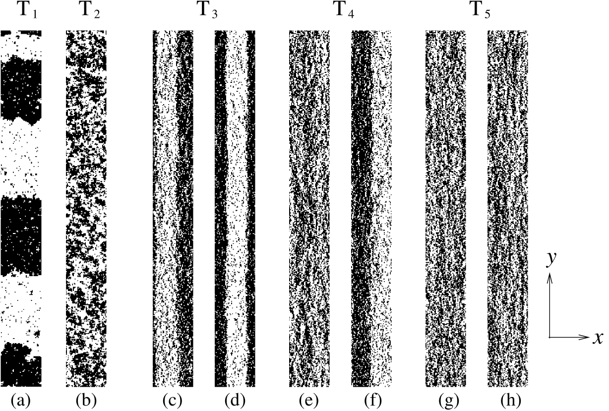
Figure 2: Typical configurations on a $48\times 432$ lattice for the equilibrium Ising model using heat bath dynamics at $T_{1}=2.00$ (a) and $T_{2}=2.80$ (b), and for its driven cousin at three temperatures: $T_{3}=2.90$ (c, d), $T_{4}=3.30$ (e, f) and $T_{5}=3.70$ (g, h). The first (second) configuration at each temperature was obtained using Metropolis (heat bath) dynamics. In each simulation, the data were collected after discarding $2\times 10^{7}$ MCS for the equilibrium system and $10^{7}$ MCS for its driven counterpart.

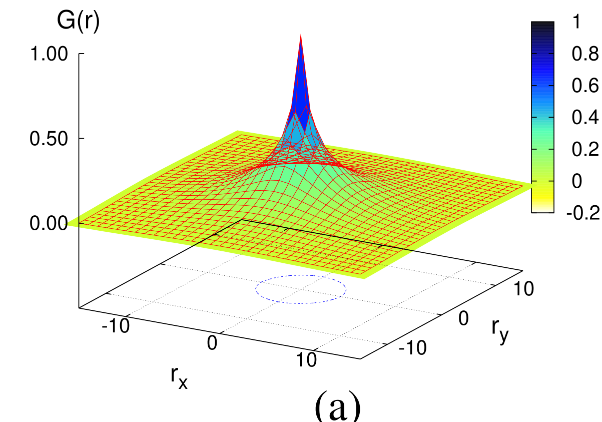
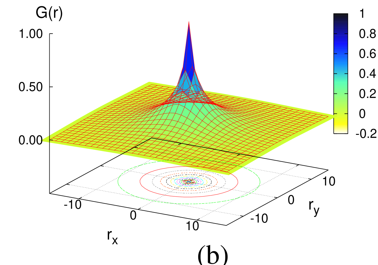
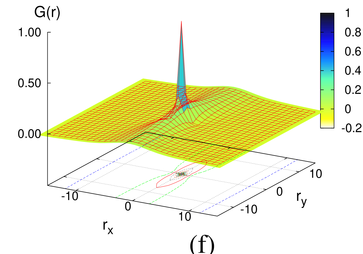
Figure 3: The pair correlation function for the equilibrium system and its driven counterpart on a $100\times 100$ lattice. The top row shows the Ising lattice gas at $T=2.47$ with Metropolis (a), heat bath (b), and Glauber (c) dynamics; the bottom row shows the driven system at $T=3.60$ with Metropolis (d), heat bath (e), and Glauber (f) dynamics.

         

Figure 4: Parallel and transverse two-point correlations for the equilibrium system at $T=2.47$ (a, b) and for the driven case at $T=3.60$ (c, d) on a $100\times 100$ lattice. Each plot shows data for three dynamics: Metropolis (asterisks), heat bath (filled squares) and Glauber (open circles). In (a, b) all data collapse, while in (c, d) only heat bath and Glauber data overlap.

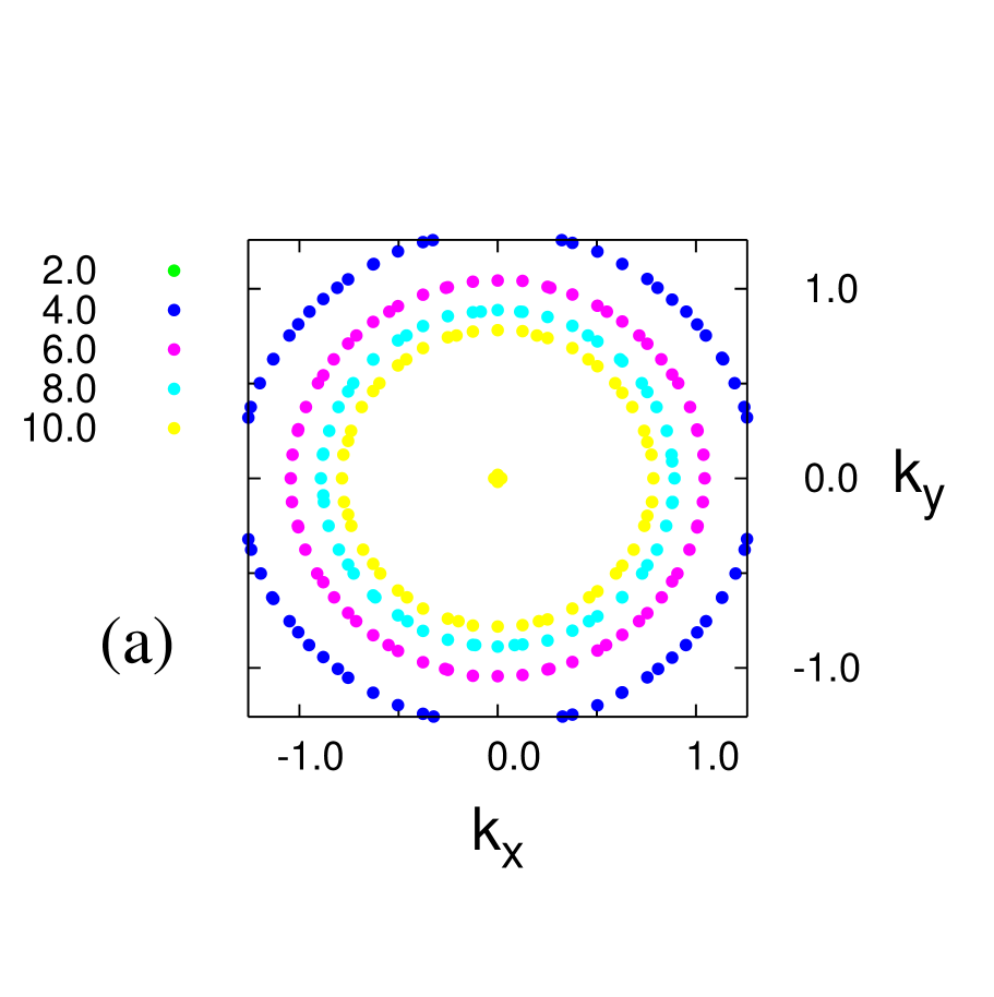
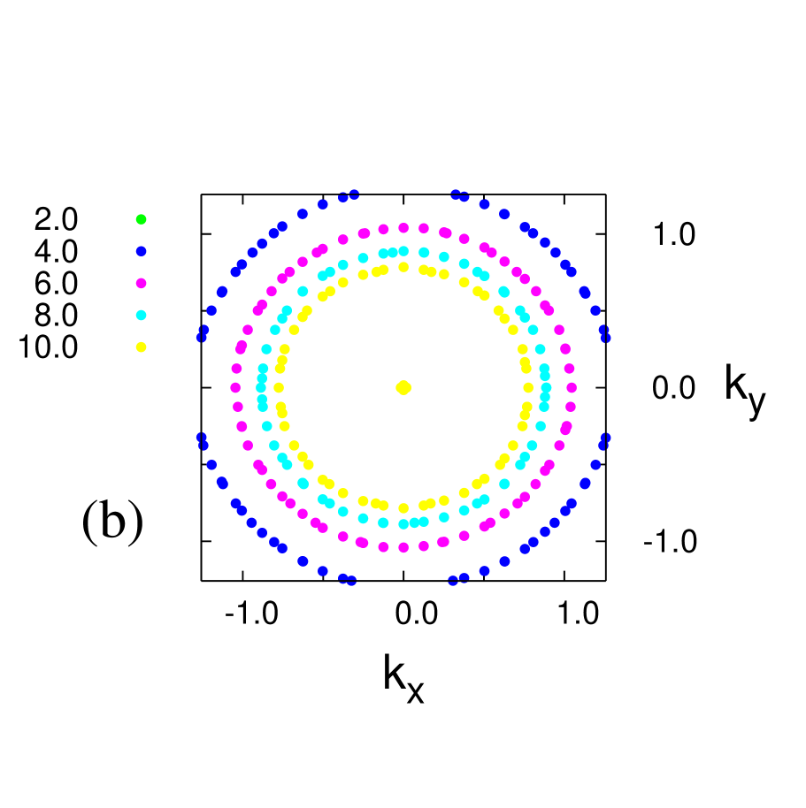
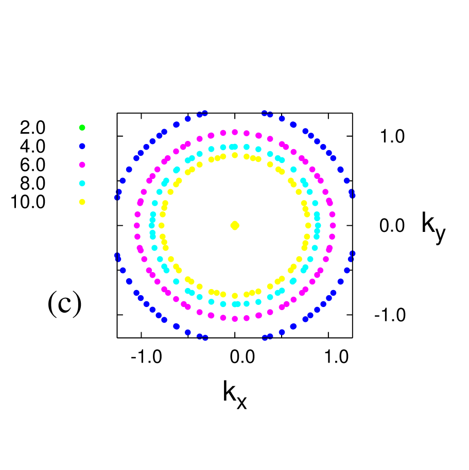
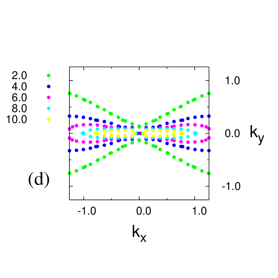
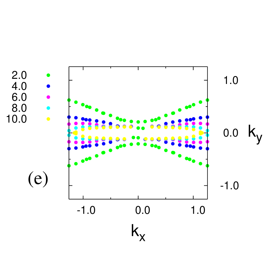
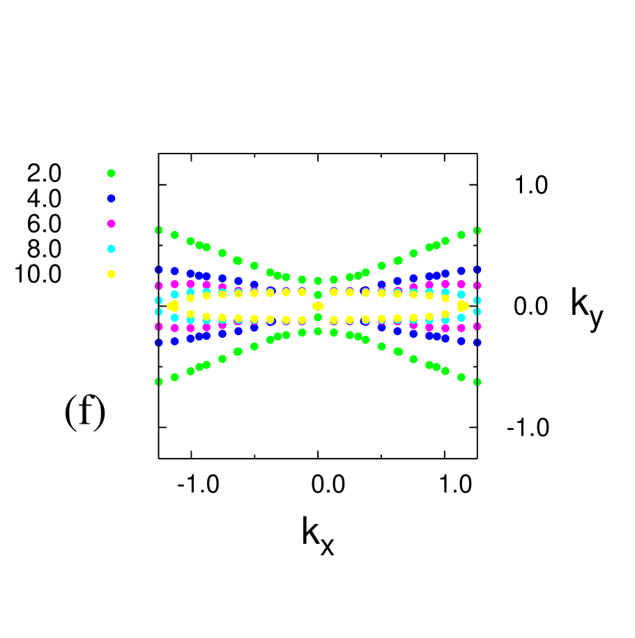
Figure 5: Structure factor contour plots for the equilibrium system and its driven counterpart on a $100\times 100$ lattice. The top row shows the Ising lattice gas at $T=2.47$ with Metropolis (a), heat bath (b), and Glauber (c) dynamics; the bottom row shows the driven system at $T=3.60$ with Metropolis (d), heat bath (e), and Glauber (f) dynamics.

         

Figure 6: Parallel and transverse structure factors for the equilibrium system at $T=2.47$ (a, b) and for the driven case at $T=3.60$ (c, d), on a $100\times 100$ lattice. Each plot shows data for three dynamics: Metropolis (asterisks), heat bath (filled squares) and Glauber (open circles). Within error bars (not shown), the data effectively collapse in (a, b), while only heat bath and Glauber data overlap in (c, d). Note the different scale in (d).

III.1 Typical configurations, two-point correlations and structure factors.

We begin our discussion by showing a few typical configurations of the driven system on a $48\times 432$ lattice. Figs. 2a and b are obtained for the equilibrium case, just below and above criticality. The preference for horizontal interfaces is clearly seen in Fig. 2a. The remaining configurations (Fig. 2c-h) all show the driven system, for heat bath and Metropolis dynamics, at three different temperatures. At the lowest temperature $T_{1}=2.90$ (Figs. 2c, d), the driven system is ordered for both dynamics. In stark contrast to the equilibrium case, the interfaces between high- and low-density regions are parallel to $\mathcal{E}$ and therefore clearly not dominated by energetics. At a slightly higher temperature, $T_{2}=3.30$ (Figs. 2e, f), we observe the first glaring discrepancy between the two dynamics: the configuration generated by the heat bath algorithm is still ordered while the Metropolis configuration is already disordered! Eventually, at $T_{3}=3.70$, both algorithms generate disordered configurations. Clearly, the two algorithms lead to different critical temperatures, with $T_{c}^{M}<$ $T_{c}^{H}$. A rough estimate based on our data WK-unpub results in $T_{c}^{H}=3.55\pm 0.05$ and $T_{c}^{M}=3.15\pm 0.05$. More precise estimates Italy are available for Metropolis rates only: $T_{c}^{M}=3.\,\allowbreak 198\,01(19)$.

To probe this apparent discrepancy between Metropolis and heat bath rates further, and to explore the position of Glauber rates in this triad, we turn to a more detailed analysis. In Fig. 3, we show surface plots of $G\left(\mathbf{r}\right)$ for the Ising lattice gas (top row, Figs. 3a-c) and the driven system (bottom row, Figs. 3d-f). The three columns correspond to the three different dynamics: Metropolis (Figs. 3a, d), heat bath (Figs. 3b, e), and Glauber (Figs. 3c, f). Fig. 4 shows selected projections of $G\left(\mathbf{r}\right)$, namely $G(0,y)$ and $G(x,0)$, for equilibrium (Fig. 4a, b) and with infinite drive (Fig. 4c, d). As dictated by detailed balance, the correlation functions for the equilibrium system are independent of dynamics: there are no discernable differences between Figs. 3a-c, and the data in Figs. 4a and b collapse within statistical error bars (less than $0.01$ in absolute units). The chosen temperature, $T=2.47$, is close enough to Ising criticality so that lattice anisotropies are irrelevant: $G\left(\mathbf{r}\right)$ is isotropic, with circular contours centered on the origin. The small negative values observed at large distances are a consequence of the sum rule.

This simple picture becomes considerably more complex when we turn to the driven system (lower row of Fig. 3 and Figs. 4c, d). The chosen temperature, $T=3.60$, is very close to our estimate for the critical temperature of heat bath and Glauber rates, $T_{c}^{H}\simeq T_{c}^{G}$ $\simeq 3.55$ and about $15\%$ above $T_{c}^{M}$. We immediately note the strong anisotropy induced by the drive. Further, there are noticeable differences between Metropolis rates on one hand, and heat bath and Glauber dynamics on the other. These are most easily observed in Figs. 4c and d. For Metropolis rates, $G^{M}(0,y)$ is positive and decreases monotonically throughout (Fig. 4c), while $G^{M}(x,0)$ drops rapidly below zero, displays a minimum and then recovers and approaches zero from below. These features have been noted before KLS , and are directly related to the breaking of detailed balance SZ ; corr'ns-anal ; discont . The data for Glauber and heat bath dynamics, while practically indistinguishable from one another, differ visibly from the Metropolis ones. Considering correlations measured along the field direction first, we observe $G^{H}(0,y)\simeq G^{G}(0,y)>G^{M}(0,y)$ for all $y$. In other words, Metropolis rates generate weaker correlations, consistent with the lower $T_{c}^{M}$. Heat bath and Glauber rates produce roughly the same correlations; moreover, these show clear signatures of being very close to criticality, evidenced by the distinctly positive value at the largest $y$ shown: $G^{H}(0,40)\simeq G^{G}(0,40)\simeq 0.07$. Highly correlated domains in the driven system are needle-shaped, with the needle pointing along the field, and this small, yet nonzero value indicates that some of these domains are long enough to span half the system. These precursors of ordering become even more obvious when we turn to correlations transverse to the field: The secondary maximum in Fig. 4d indicates a tendency towards forming thin stripes for heat bath and Glauber rates.

The structure factors bear out this picture. Again, the independence from the rates, and the isotropy near criticality is clearly displayed by the contour plots for the equilibrium system, shown in Figs. 5a-c, and by the projections shown in Figs. 6a, b. In the driven case (Figs. 5d-f and 6c, d), the presence of strong anisotropy is apparent, and the well-known discontinuity singularity at the origin discont is observed easily: $\lim_{k_{x}\rightarrow 0}S(k_{x},0)\neq\lim_{k_{y}\rightarrow 0}S(0,k_{y})$. While these broad features characterize all three dynamics, the absolute values of the structure factors differ slightly from one another: $S^{M}(k_{x},k_{y})$  is generally smaller than either $S^{H}(k_{x},k_{y})$ or $S^{G}(k_{x},k_{y})$. Moreover, the distance from criticality can be measured through the discontinuity ratio,

$$\mathcal{S}\equiv\frac{\lim_{k_{x}\rightarrow 0}S(k_{x},0)}{\lim_{k_{y}\rightarrow 0}S(0,k_{y})}$$

which diverges as $T\rightarrow T_{c}$ discont . Our data result in $\mathcal{S}^{M}\simeq 7.5$, while $\mathcal{S}^{H}\simeq\mathcal{S}^{G}\simeq 34>\mathcal{S}^{M}$. Our findings confirm, once again, that the heat bath and Glauber data are effectively much closer to criticality than those for Metropolis rates.

Figure 7: Normalized histograms for the equilibrium system using heat bath (solid line) and Metropolis (dotted line) rates, at $\beta_{1}=1/2.269$ (a) and $\beta_{2}=1/2.369$ (b). In (c), we show $\ln R_{0}$ vs $E-E^{\prime}$: Data are shown as open (Metropolis) and filled (heat bath) squares; the solid line is the expected behavior, $-(\beta_{1}-\beta_{2})(E-E^{\prime})$.

Figure 8: Normalized histograms for the driven system using heat bath (solid line) and Metropolis (dotted line) rates, at $\beta_{1}=1/3.550$ (a) and $\beta_{2}=1/3.650$ (b). In (c), we show $\ln R_{\mathcal{\infty}}$ vs $E-E^{\prime}$. Metropolis data are shown as open circles and are taken at $\beta_{1}=1/3.200$ and $\beta_{2}=1/3.300$; the heat bath data (filled circles) are taken at $\beta_{1}^{\prime}=1/3.550$ and $\beta_{2}^{\prime}=1/3.650$. Two theoretical lines are shown: $-(\beta_{1}-\beta_{2})(E-E^{\prime})$ (dotted) and $-(\beta_{1}^{\prime}-\beta_{2}^{\prime})(E-E^{\prime})$ (solid).

III.2 Histogram Ratio Analysis

In the final section, we turn to a brief investigation of energy histograms. Since Glauber and heat bath rates produce essentially identical data, we restrict ourselves in the following to just heat bath and Metropolis rates. To set the scene, we first show two histograms for the equilibrium system, generated at, and slightly above, criticality: $T_{1}=2.269$ and $T_{2}=2.369$ (Figs. 7a and b, respectively). As expected, the data for the different dynamics collapse very well, within statistical errors. Not surprisingly, the peak position shifts to higher energies with increasing temperature, while the width is largest at criticality. In Fig. 7c, we plot the corresponding histogram ratio, Eq. (15), and compare it to the predicted exponential form. The agreement is of course very good.

With Fig. 8, we enter novel territory. In analogy to the equilibrium plots, Figs. 8a and b display the energy histograms of the driven system, at two temperatures, $T_{1}=3.550$ and $T_{2}=3.650$, for heat bath and Metropolis dynamics. The chosen temperatures correspond to criticality and slightly above for heat bath rates; for Metropolis rates, both are well inside the disordered phase. In contrast to the equilibrium case, the histograms clearly depend on the choice of rates: the peak positions are considerably higher for Metropolis than for heat bath rates. At the same time, the width is largest for the system closest to criticality, i.e., $T_{1}=3.550$ with heat bath rates.

A comment is in order, concerning the judicious choice of the two temperatures which enter the histogram ratio. It applies to both the equilibrium and the driven case. As we can see from Figs. 7 and 8, each histogram displays a well-developed peak. Energies far away from the peak position occur rarely, so that histograms are plagued by large statistical errors in those regions. In order to yield a reliable ratio, the corresponding histograms should overlap in their statistically meaningful domains. Hence, the two chosen temperatures must not lie too far apart.

In Fig. 8c, we present the histogram ratio for the driven system. For each dynamics, two temperatures close to their respective critical temperatures were chosen: $3.200$ and $3.300$ for Metropolis rates, and $3.550$ and $3.650$ for heat bath rates. Remarkably, we observe that the histogram ratio for both is again a simple exponential, i.e., $\ln R_{\mathcal{\infty}}(E,E^{\prime})\propto(E-E^{\prime})$, at least over the range shown. In stark contrast to the equilibrium case, there is no a priori reason here to expect such behavior. Instead, it indicates that $F(E,\beta)$ in Eq. (16) depends sufficiently smoothly on $E$ as to allow an expansion in $\Delta\equiv E-E^{\prime}$:

$$\ln R_{\mathcal{\infty}}(E,E^{\prime}) = -\Delta\left[\frac{\partial F(E,\beta_{1})}{\partial E}-\frac{\partial F(E,\beta_{2})}{\partial E}\right]+O(\Delta^{2})$$ (17)

$$\equiv -\alpha\Delta+O(\Delta^{2})$$

Hence, the slope of the data in Fig. 8c allows us to probe $\alpha$, as a function of temperature and dynamics. It manifestly differs from the equilibrium form $(\beta_{1}-\beta_{2})$. A more systematic study is required to extract, and interpret, its properties.

IV Conclusions

We have simulated the equilibrium Ising lattice gas and its driven non-equilibrium counterpart, using three different dynamics: Metropolis, Glauber and heat bath. In the equilibrium case, all three rate functions satisfy detailed balance with respect to the Ising Hamiltonian; as a consequence, all stationary (time-independent) equilibrium quantities are expected to be independent of the choice of the dynamics. Apart from unavoidable statistical errors, our equilibrium data are of course perfectly consistent with this expectation. For the driven system, this is no longer the case: due to the drive, all three rate functions violate detailed balance, and the ‘decoupling’ of stationary properties from the chosen dynamics no longer holds. Measuring two-point correlations and structure factors in the disordered phase, we observe distinct differences between the three dynamics. On the one hand, Metropolis rates lead to a lower critical temperature, and hence generally weaker correlations in the disordered phase, than either Glauber or heat bath rates. On the other hand, the latter two generate practically indistinguishable data. These features can be understood in terms of a few basic properties of the three rates: At a given temperature, Metropolis rates tend to accept all moves with a somewhat higher probability than the other two rate functions. In other words, a system which evolves under the Metropolis algorithm ‘sees’ an effectively higher temperature than if it were running under heat bath or Glauber. A similar observation was made recently for field-driven Ising or solid-on-solid interfaces, subject to Glauber and Metropolis dynamics: there, Metropolis rates appear to lead to rougher interfaces and higher propagation velocities than Glauber rates PAR . In contrast, heat bath and Glauber rates partition the unit interval into the same subsections and accept/reject moves according to this partition. As a result, they generate statistically indistinguishable trajectories in configuration space, leading to essentially identical data.

It is essential to note, however, that the broad characteristics, associated with the breaking of detailed balance, are clearly observed in all three dynamics: all structure factors show the typical discontinuity singularity at the origin which, in turn, translates into power law decays of the two-point correlation functions. To summarize, universal features, associated with global symmetries, remain independent of local changes of dynamic rules, both near and far from equilibrium.

In a second part of this paper, we discuss the energy histograms $H(E,\beta)$ associated with our two models, generated by heat bath and Metropolis dynamics. For the equilibrium system, the independence of the choice of dynamics is borne out again, while differences emerge in the driven case. A simple ratio, $R(E,E^{\prime})$, constructed from two histograms measured at different temperatures $\beta_{1}$ and $\beta_{2}$, allows us to probe their functional form for a specified dynamics. In equilibrium, the canonical distribution prescribes a simple exponential dependence, $\ln R_{0}=-(\beta_{1}-\beta_{2})(E-E^{\prime})$. Remarkably, its non-equilibrium counterpart $\ln R_{\infty}$ is also exponential in $(E-E^{\prime})$. This behavior indicates a smooth dependence of $F(E,\beta)\equiv-\ln H(E,\beta)$ on $E$, allowing us to linearize $\ln R_{\mathcal{\infty}}$ in $(E-E^{\prime})$. The slope of the resulting straight line depends on the dynamics and probes the derivative $(\partial F/\partial E)$. Further, and more detailed, studies of this type may reveal some of the hidden “thermodynamics” of this remarkably complex non-equilibrium steady state.

V Acknowledgment

We thank Royce K.P. Zia and Per A. Rikvold for fruitful discussions. This research was supported in part by National Science Foundation Grants No. DMF-0094422 and DMR-0088451.

References

- (1) For reviews, see, e.g., Computer Simulation Studies in Condensed Matter Physics II, eds. D. P. Landau, K. K. Mon, and H.-B. Schüttler (Springer-Verlag, Berlin, 1990); K. Binder, Computational Methods in Field Theory, eds. C. B. Lang and H. Gausterer, (Springer, Berlin, 1992); K. Binder and D. W. Heermann, Monte Carlo Simulation in Statistical Physics, (Springer, Berlin, 1992).
- (2) R. H. Swendsen, J.-S. Wang, Phys. Rev. Lett. 58, 86 (1987).
- (3) B. Schmittmann and R.K.P Zia, Statistical Mechanics of Driven Diffusive Systems, Vol 17 of Phase Transitions and Critical Phenomena, eds. C. Domb and J.L. Lebowitz (Academic Press, London, 1995).
- (4) D. Mukamel, in Soft and Fragile Matter: Non-Equilibrium Dynamics, Metastability and Flow, eds. M.E. Cates and M.R. Evans (Institute of Physics Publishing, Bristol, 2000); J. Marro and R. Dickman, Non-Equilibrium Phase Transitions in Lattice Models (Cambridge University Press, Cambridge, 1999).
- (5) S. Katz, J. L. Lebowitz, and H. Spohn, Phys. Rev. B 28, 1655 (1983) and J. Stat. Phys. 34, 497 (1984).
- (6) J. Krug, J.L. Lebowitz, H. Spohn, and M.Q. Zhang, J. Stat. Phys. 44, 535 (1986); R. Dickman, Phys. Rev. A38, 2588 (1988).
- (7) N. Metropolis, A.W. Rosenbluth, M.M. Rosenbluth, A.H. Teller, and E. Teller, J. Chem. Phys. 21, 1087 (1953).
- (8) R. J. Glauber, J. Math. Phys. 4, 294 (1963).
- (9) M. Creutz, Phys. Rev. D 21, 2308 (1980).
- (10) The only exception, to the best of our knowledge, is an anisotropic generalization of Metropolis rates: J.L. Vallés and J. Marro, J. Stat. Phys. 43, 441 (1986); I. Mazilu, Steady state properties of some driven diffusive systems, PhD thesis (Virginia Tech, Blacksburg 2002) http://scholar.lib.vt.edu/theses/available/etd-09022002-101837/
- (11) H. van Beijeren and L.S. Schulman, Phys. Rev. Lett. 53, 806 (1984); J. Krug and H. Spohn, in Nonlinear Evolution and Chaotic Phenomena, eds. G. Gallavotti and P.F. Zweifel, NATO ASI Series B Vol 176 (Plenum Press, New York 1988); I. Mazilu and B. Schmittmann, J. Stat. Phys. 113, 505 (2003).
- (12) Alan M. Ferrenberg, R. H. Swendsen, Phys. Rev. Lett. 61, 2635 (1988); Alan M. Ferrenberg, D. P. Landau, and Robert H. Swendsen, Phys. Rev. E 51, 5092 (1995).
- (13) R.K.P. Zia and T. Blum, in Scale Invariance, Interfaces, and Non-Equilibrium Dynamics, eds. A. McKane, M. Droz, J. Vannimenus, and D. Wolf, NATO ASI Series B Vol 344 (Plenum Press, New York 1995).
- (14) L. Onsager, Phys. Rev. 65, 117 (1944); B.M. McCoy and T.T. Wu, The Two-dimensional Ising Model (Harvard University Press, Cambridge, MA, 1973).
- (15) W. Kwak and D.P. Landau, unpublished.
- (16) S. Caracciolo, A. Gambassi, M. Gubinelli, and A. Pelissetto, J. Phys. A 36, L315 (2003), and J. Stat.Phys. 115, 281 (2004).
- (17) M.Q. Zhang, J.-S. Wang, J.-L. Lebowitz, and J.L. Vallés, J. Stat. Phys. 52, 1461 (1988); P.L. Garrido, J.L. Lebowitz, C. Maes, and H. Spohn, Phys. Rev. A 42, 1954 (1990).
- (18) R.K.P. Zia, K. Hwang, K.-t. Leung and B. Schmittmann, in: Computer Simulation Studies in Condensed Matter Physics V, eds D.P. Landau, K.K. Mon and H.B. Schüttler (Springer, Berlin 1993); R.K.P. Zia, K. Hwang, B. Schmittmann and K.-t. Leung, Physica A 194, 183 (1993).
- (19) P.A. Rikvold and M. Kolesik, J. Stat. Phys. 100, 377 (2000).