Spin-torque switching: Fokker-Planck rate calculation

Abstract

We describe a new approach to understanding and calculating magnetization switching rates and noise in the recently observed phenomenon of ”spin-torque switching”. In this phenomenon, which has possible applications to information storage, a large current passing from a pinned ferromagnetic (FM) layer to a free FM layer switches the free layer. Our main result is that the spin-torque effect increases the Arrhenius factor $\exp(-E/kT)$ in the switching rate, not by lowering the barrier $E$, but by raising the effective spin temperature $T$. To calculate this effect quantitatively, we extend Kramers’ 1940 treatment of reaction rates, deriving and solving a Fokker-Planck equation for the energy distribution including a current-induced spin torque of the Slonczewski type. This method can be used to calculate slow switching rates without long-time simulations; in this Letter we calculate rates for telegraph noise that are in good qualitative agreement with recent experiments. The method also allows the calculation of current-induced magnetic noise in CPP (current perpendicular to plane) spin valve read heads.

I Introduction

Recently it has been demonstrated that the magnetization of a thin ferromagnetic film can be switched by passing a current between it and a pinned layeralbert . This ”spin-torque switching” phenomenon is of interest for possible information storage applications. Except at very high currents, the switching appears to be thermal in nature. Previous theoretical treatments of thermal spin-torque switchingmyers ; zhang ; zhangXXX have been based on the idea that the spin torque increases the rate by lowering the effective potential energy barrier, and have encountered a fundamental problem: the common Slonczewskislon96 ; slon99 model for the spin torque is not conservative, so it cannot be described by a potential energy. The effects of the Slonczewski torque on the Landau-Lifshitz (LL) equation for the magnetization dynamics are similar to those of the LL damping, so in our Fokker-Planck approach it makes a contribution to the effective damping. When this contribution is negative, the effective temperature is raised. The notion of an elevated effective temperature during spin-torque switching has been discussed previouslyurazhdin ; wegrowe ; koch ; the present Fokker-Planck formulation allows the precise definition and calculation of the effective temperature, which we will refer to as the Maxwell-Boltzmann temperature (Eq. 16) and clarifies the relation between it and the (lower) LL noise temperature.

The Fokker-Planck equation gives the time evolution of a phase space probability density. It was first applied to chemical rate problems in 1940 by Kramerskramers , who observed that except for very large or very small damping constants, the escape rate is well described by an earlier ”transition state theory” (TST)eyring , in which the rate of barrier-crossing in a non-equilibrium system is assumed to be the same as that in an equilibrium system.  Although corrections to TST have been extensively studiedchandler ; visscher , TST has been found to be the most useful starting point for rate calculations.  In this Letter we will use a TST-like approximation, differing from the usual TST in that the system is not in a true thermal equilibrium, but a non-equilibrium steady state.  We will write the magnetic Fokker-Planck equation of Brownbrown , generalized to include the Slonczewski torque, but following Kramerskramers convert it to describe diffusion in energy rather than magnetization; to the best of our knowledge this has not been done previously except for systems with azimuthal symmetrybrown ; coffey .

The LL equationgeneral for the evolution of a uniform magnetization $\mathbf{M}(t)$ has a deterministic and a random part:

$$\dot{\mathbf{M}}{\equiv}\frac{d{{\mathbf{M}}}}{dt}=\dot{\mathbf{M}}_{\text{det}}+\dot{\mathbf{M}}_{\text{rand}}$$ (1)

The deterministic part is divided into a conservative precession term and the dissipative LL damping, and we will include also the Slonczewski current-induced torque:

$$\dot{\mathbf{M}}_{\text{det}}=\dot{\mathbf{M}}_{\text{cons}}+\dot{\mathbf{M}}_{\text{LL}}+\dot{\mathbf{M}}_{\text{Slon}}$$ (2)

We will first specify the precession torque:

$$\dot{\mathbf{M}}_{\text{cons}}=-\gamma\mathbf{M}\times\mathbf{H}_{\text{cons}}$$ (3)

where $\gamma$ is the gyromagnetic ratio.  We refer to the field $\mathbf{H}_{\text{cons}}$ about which $\mathbf{M}$ precesses as ”conservative” because it can be written as the gradient with respect to $\mathbf{M}$ of an energy density,

$$\mu_{0}\mathbf{H}_{\text{cons}}=-\nabla E(\mathbf{M)}.$$ (4)

(This is a 2D gradient on the $\mathbf{M}$-sphere; see Eq. 25 of ref. epaps .)

Our derivation of the FP equation is valid for a system with arbitrary anisotropy, but for specificity we will consider the case of a thin-film element (Fig. 1)

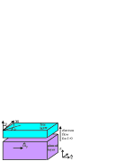
Figure 1: Geometry of thin-film element, for the case where the magnetization $\hat{\mathbf{m}}_{\text{p}}$ of the ”pinned” layer is along the easy axis $\hat{\mathbf{e}}$ of the free layer.

for which the energy density is given (in SI units) bygeneral

$$E(\mathbf{M})/\mu_{0}=-\frac{1}{2}H_{K}M_{s}\mathbf{{(\hat{{m}}\cdot\hat{e})}}^{2}+\frac{1}{2}M_{s}^{2}\mathbf{{(\hat{{m}}\cdot\mathbf{\hat{z}})}}^{2}-\mathbf{{{H}_{\text{ext}}\cdot\mathbf{M}}}$$ (5)

Here $\mathbf{{{H}_{\text{ext}}}}$ is an external field, $H_{K}$ is the uniaxial anisotropy field, $\mathbf{\hat{m}\equiv M}/M_{s}$, $\mathbf{\hat{e}}$, and $\mathbf{\hat{z}}$ are unit vectors along the magnetization, easy axis, and z axis (perpendicular to the film) respectively, and $M_{s}$ is the saturation magnetization.

The nonconservative LL damping torque (Eq. 2) isgeneral

$$\dot{\mathbf{M}}_{\text{LL}}\mathbf{=-}\gamma\alpha M_{s}\hat{\mathbf{m}}\times(\hat{\mathbf{m}}\times\mathbf{H}_{\text{cons}})=\gamma\alpha M_{s}\mathbf{H}_{\text{cons}}$$ (6)

where $\alpha$ is the dimensionless LL damping constant.  The Slonczewski spin-torqueslon99 ; zhang is

$$\dot{\mathbf{M}}_{\text{Slon}}=-\gamma JM_{s}\hat{\mathbf{m}}\times(\hat{\mathbf{m}}\times\hat{\mathbf{m}}_{\text{p}})$$ (7)

where $J$ is an empirical constant with units of magnetic field, proportional to the current density, and $\mathbf{{\hat{{m}}}_{\text{p}}}$ is the magnetization direction in the thicker (often pinned) layer from (or to) which the current flows.

The effect of the random torque $\dot{\mathbf{M}}_{\text{rand}}$ is to produce a diffusive random walk on the surface of the $\mathbf{M}$-sphere.  We will relate this to a diffusivity $D$ (Eq. 18) by giving the mean square value of the increment $\Delta\mathbf{M}_{\text{rand}}=\dot{\mathbf{M}}_{\text{rand}}\Delta t$:

$$\left\langle\Delta\mathbf{M}_{\text{rand}}^{2}\right\rangle=4D\Delta t.$$ (8)

The directions of these torques are shown in insets to Fig. 2, from which the basic mechanism of spin-torque switching can be seen: the Slonczewski torque pulls the magnetization out of well $1$ and allows it to jump to well $2$.

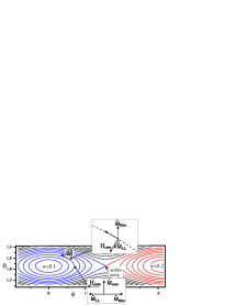
Figure 2: Energy contours (Stoner-Wohlfarth orbits) for a thin film, plotted in terms of the coordinates $\theta$ and $\phi$ defined in Fig. 1, for the case $H_{K}/M_{s}{=0.028}$, $\mathbf{{{H}_{\text{ext}}}}=0.$ The regions $i=1,2,3$ are blue, red, and black respectively. The vertical scale is exaggerated for clarity.  Lower inset: contributions to the rate of change of magnetization for a magnetization in the film plane.  The insets show the tangent plane: magnetization points out of the paper.  Upper inset: the same for an arbitrarily chosen direction of $\mathbf{M}$.

The Fokker-Planck equation describes the evolution of a probability density $\rho(\mathbf{M},t)$ on the $\mathbf{M}$-sphere. It can be written in the form of a continuity equationbrown for $\rho(\mathbf{M},t)$:

$$\frac{\partial\rho(\mathbf{M},t)}{\partial t}=-\nabla\cdot\mathbf{j}(\mathbf{M},t)$$ (9)

where the probability current $\mathbf{j}$ along the sphere has a convective and a diffusive part:

$$\mathbf{j}(\mathbf{M},t)\equiv\rho(\mathbf{M},t)\dot{\mathbf{M}}_{\text{det}}(\mathbf{M})-D\nabla\rho(\mathbf{M},t)$$ (10)

(note that both the divergence and the gradient are two-dimensional here).  Inserting Eq. 10 into Eq. 9 gives the FP equation (Eq. 26 of ref. epaps ) first derived (without the spin torque term) in 1963 by Brownbrown .

Frequently, the probability density depends mostly on energy, being constant along an orbit and depending weakly on phase around the orbit.  This is exactly true in a thermal equilibrium system (even with damping), and we show below that it is true in a steady state system with a Slonczewski torque, modeling the telegraph noise system.  It has often been assumed to be approximately true away from the barrier, to compute non-equilibrium switching rateskramers ; brown ; coffey .  The energy dependence may be different in different regions of the sphere (for example, different energy wells), so we will define a density $\rho_{i}^{\prime}(E,t)$, where the region (well) index $i=1$ for the $\phi=0$ well (for $E\leq E_{\text{sad}}$), $i=2$ for the $\phi=\pi$ well (Fig. 2), and $i=3$ for $E\geq E_{\text{sad}}$.  [The three will be equal at the saddle point, where all three regions touch.]  This density $\rho^{\prime}$ is related to $\rho_{i}$ by

$$\rho(\mathbf{M},t)=\rho_{i}^{\prime}(E(\mathbf{M)},t)$$ (11)

Kramers derived a Fokker-Planck equation in energy for a particle in a well, but we are not aware of any previous derivation for the magnetic case so we will derive it here. Though Kramers used it only in the low-damping limit, it is an exact description of the steady state of the system even for high damping.

The FP equation in energy takes the form of a continuity equation

$$\frac{\gamma M_{s}P_{i}(E)}{\mu_{0}}\frac{\partial\rho_{i}^{\prime}(E,t)}{\partial t}=-\frac{\partial}{\partial E}j_{i}^{E}(E,t)$$ (12)

where the current $j_{i}^{E}(E,t)$ is the number of systems per unit time crossing a constant-energy contour.  There is a factor on the left hand side involving the orbital period $P_{i}(E)$ because $\rho^{\prime}$ is not the probability per unit energy but per unit area on the $M$-sphere (see Eq. 47 of ref. epaps ).  The current in energy can be obtained from the current on the $M$-sphere (Eq. 10; see Eqs. 28-37 of ref. epaps for details):

$$j_{i}^{E}(E,t)=-\gamma\alpha M_{s}\rho_{i}^{\prime}(E,t)I_{i}(E)+\gamma JM_{s}\rho_{i}^{\prime}(E,t)\hat{\mathbf{m}}_{\text{p}}\cdot\mathbf{I}_{i}^{M}-D\frac{\partial\rho_{i}^{\prime}(E,t)}{\partial E}I_{i}(E)$$ (13)

in terms of a damping term involving an energy integral over an orbit in the $i^{\text{th}}$ well

$$I_{i}^{E}(E)\equiv\oint H_{\text{cons}}dM,$$ (14)

a Slonczewski torque term involving a magnetization integral

$$\mathbf{I}_{i}^{M}(E,t)=\oint d\mathbf{M}\times\mathbf{M}$$ (15)

and a diffusion term.

For the telegraph-noise problem we require the steady-state form obtained by setting $j_{i}^{E}=0$:

$$\frac{\partial\ln\rho^{\prime}(E)}{\partial E}=\frac{\gamma}{D}\left[-\alpha M_{s}+\eta(E)J\right]\equiv-V\beta(E)$$ (16)

where the right hand side defines an effective inverse ”Maxwell-Boltzmann” temperature $\beta(E)$, and $V$ is the volume of the switching element. We have also defined a dimensionless spin-torque-damping ratio $\eta(E)$ (Fig. 3) as the ratio of the work of the Slonczewski torque (Eq. 7) to that of the LL damping (Eq. 6)

$$\eta(E)=\frac{\hat{\mathbf{m}}_{\text{p}}\cdot\mathbf{I}_{i}^{M}(E)}{I_{i}^{E}(E)}.$$ (17)

Eq. 16 shows clearly that the Slonczewski torque acts like a correction to the LL damping $\alpha$.  Because $\eta$ has opposite signs in the two wells, the damping contribution is negative in one well and positive in the other.  A similar result has been suggested previouslykoch for the special case in which $\hat{\mathbf{m}}_{\text{p}}$ is parallel to $\mathbf{H_{\text{ext}}}$.

If $J=0$, we get the expected Boltzmann distribution with $\beta=1/k_{B}T$ only if

$$D=\gamma M_{s}\alpha k_{B}T/V;$$ (18)

this is the fluctuation-dissipation theorem.

If we integrate Eq. 16 downward from the saddle point into well $i=1$ or 2, we get

$$\rho_{i}^{\prime}(E)=\rho^{\prime}(E_{\text{sad}})\exp\left[\frac{V}{k_{B}T}[1-\overline{\eta_{i}}(E)J/\alpha M_{s}][E_{\text{sad}}-E]\right]$$ (19)

where the average $\eta$ is

$$\overline{\eta}_{i}(E)\equiv\frac{1}{[E_{\text{sad}}-E]}\int\limits_{E}^{E_{sad}}\eta_{i}(E^{\prime})dE^{\prime}$$ (20)

In region $i=3$ we must integrate upwards from $E_{\text{sad}}$ (see Eq. 44 of ref. epaps ).  The ratio $\eta$ and its average $\overline{\eta}$ are weakly dependent on $E$ (Fig. 3), so the distribution is nearly a Boltzmann distribution with an effective temperature $T/[1-\overline{\eta}(E)J/\alpha M_{s}]$.

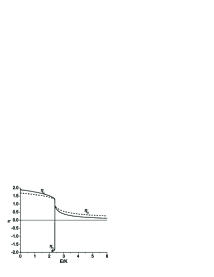
Figure 3: The current-damping coefficients $\eta_{1}$ and $\eta_{2}$ in the two potential wells, and $\eta_{3}$ for the region above the saddle-point energy. The values we actually use (near the bottoms of the wells) depend only weakly on the parameters $H_{\text{ext}}=-120$ Oe and $H_{K}=220$ Oe, which were estimated from the fit to experimental data (Eq. 52 of ref. epaps ). The averages $\overline{\eta}_{i}$ (Eq. 20) are also shown, as dashed lines.

We now compute the switching rates using transition state theory (TST). The TST rate is the steady-state probability per unit time of crossing a vertical line ($\phi=\pi/2$) through the saddle point in Fig. 2. This givesepaps

$$j_{\text{TST}}=\frac{\gamma M_{s}k_{B}T}{\mu_{0}V[1-\overline{\eta_{3}}(E_{\text{sad}})J/\alpha M_{s}]}\rho^{\prime}(E_{\text{sad}})$$ (21)

From the $\rho_{i}^{\prime}$s (Eq. 19) it is straightforward to obtain the total probability $p_{i}$ of being in each well (Eq. 49 of ref. epaps ).  With the absolute-rate-theory current $j_{\text{TST}}$ (Eq. 21) these determine the dwell times $\tau_{1}$ and $\tau_{2\text{ }}$.We will write these in terms of a stability factor $S_{i}\equiv VE^{b}_{i}/k_{B}T$ ($E^{b}_{i}$ is the barrier height $E_{\text{sad}}-E_{i}$, where $E_{i}$ is the bottom of well $i=1$ or $2$) and a critical current at which the exponent in Eq. 19 vanishes, $J_{ci}\equiv\alpha M_{s}/\overline{\eta_{i}}(E_{i})$.  Since we do not know the exact proportionality factor between the parameter $J$ and the actual physical current $I$ we can write $J/J_{ci}$ as $I/I_{ci}$, where the critical currents $I_{ci}$ should be related by

$$I_{c1}\overline{\eta_{1}}(E_{1})=I_{c2}\overline{\eta_{2}}(E_{2})=I_{c3}\overline{\eta_{3}}(E_{\text{sad}})$$ (22)

Then the dwell times are given byepaps

$$\tau_{i}=\frac{p_{i}}{j_{\text{TST}}}=P_{i}(E_{i})\frac{1-I/I_{c3}}{1-I/I_{ci}}\left[e^{S_{i}(1-I/I_{ci})}-1\right]$$ (23)

We define an ”Arrhenius-Neel” approximation by neglecting $I$ in the prefactor and the $-1$:

$$\tau_{i}^{A-N}=P_{i}(E_{i})e^{S_{i}(1-I/I_{ci})}$$ (24)

so that the dwell time is just a straight line on a logarithmic plot of $\tau$ (Figure 4).  We adjust the two parameters $S_{1}$ and $I_{c1}$ to match the slope and value of the measuredurazhdin dwell time at the current $I=4.4$ ma at which $\tau_{1}$ and $\tau_{2}$ cross.  In the Arrhenius-Neel approximation, these constants have simple graphical interpretations: $I_{c1}$ is the current at which $\tau_{1}$ intersects the horizontal line at the prefactor $P_{i}$ (the orbit period), and $S_{1}$ is the (logarithmic) height of the dwell time above this prefactor at zero current.

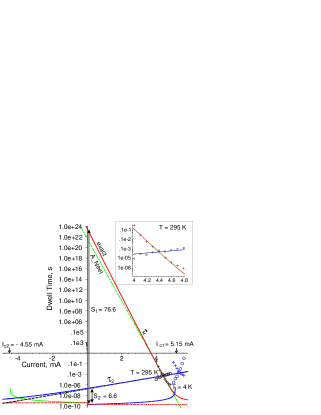
Figure 4: Dwell times as functions of current, illustrating the fitting of the room-temperature data of Urazhdin et alurazhdin .  Inset (upper right) shows the experimental points ($+$ for $\tau_{1}$, o for $\tau_{2}$) more clearly. The exact results are solid lines, the Arrhenius-Neel approximation is dotted.  Dotted horizontal lines at the bottom are the orbit periods ($P_{1\text{ }}$ on the right, $P_{2\text{ }}$ on the left).  Solid curves that approach them at $I=0$ are the prefactor $P_{i\text{ }}(1-I/I_{c3})/(1-I/I_{ci})$, which intersects the exact $\tau_{i}$ at $I_{ci}$. We use $I_{c3}=I_{c1}\overline{\eta_{1}}/\overline{\eta_{3}}$.

It can be seen from Figure 4 that the experimental data determine $I_{c1}$ quite accurately, within a few percent, because we don’t have to extrapolate very far from the experimental region to reach the prefactor curve.  On the other hand, this procedure clearly will not work for determining $I_{c2}$, because we are extrapolating from positive to negative current, and a tiny change in assumed slope causes a huge change in $I_{c2}$.  Thus we determine $I_{c2}$ from Eq. 22 instead, and then adjust $S_{2}$ to give the right value of $\tau_{2}$ at the crossing point.  The inset to Fig. 4 shows that this gives good semiquantitative agreement with the experimental data.  Although we forced the slope of $\tau_{1}$ to agree, the fact that the slope of $\tau_{2}$ is much smaller is a true prediction of the theory.

In addition to the room temperature data we fit in Fig. 4, Urazhdin et alurazhdin also measured dwell times at $T=4$K.  We show this data in Fig. 4 but it cannot be fit well by the theory.  The reason for this can be seen graphically – because the slopes of $\tau_{1}$ and $\tau_{2}$ are similar and fairly large, both will intersect the prefactor line at positive current, which is inconsistent with the model.  It has been suggestedurazhdin that an effective LL noise temperature which is different in the two wells (this could be due to Joule heating or spin-wave excitation) could explain this, but the present graphical construction suggests that this is not possible – some other mechanism must be involved.

The theory developed here is also applicable to the calculation of magnetic noise in read headsmicrowave ; simulationsperiodic of such systems show large, apparently chaotic fluctuations under some circumstances, which are predicted by the present theory as $I\rightarrow I_{c1}$.

Appendix A EPAPS Supplementary Material

A.1 Basics of the Fokker-Planck (FP) equation

The Kramers approach to chemical rate theory was adapted to the magnetic switching problem by Brownbrown , who wrote a FP equation for a probability density $\rho(M,t)$ on the sphere of possible values for the magnetization $M$ (its magnitude is assumed constant at its saturation value $M_{s}$).  In magnetic systems, the role of ”friction” is played by the Landau-Lifshitz damping coefficient $\alpha$.  Physically occurring values of $\alpha$ are low enough (about 0.01 to 0.1) that the system nearly follows a constant-energy contour (one of the closed orbits of the undamped system) and there is a slow diffusion in energy.  Brown and otherscoffey who have used the FP equation have dealt mostly with the case of non-equilibrium switching, in which one must specify an initial ensemble with all systems in one of the two potential wells, and details of the construction of this initial ensemble can strongly affect the resulting rate.  If the damping is weak, the rate may be slower than TST due to delay in reaching equilibrium near the barrier (this can lead to a rate proportional to the damping coefficient in this limitkramers brown )  It is worth noting that the telegraph noise problem is in some ways simpler, since we can deal with a steady-state distribution, and the damping-independent TST rate is always a good approximation for physical values of $\alpha$.

If $\alpha$ is large, we should use the Gilbert formulationgeneral and replace $\gamma$ by $\gamma/(1+\alpha^{2})$, in Eqs. 3 and 6, but here we take $\alpha$ to be small.

A.2 Defining temperatures in a magnetic system

In a magnetic system one must make distinctions among several different temperatures.  Clearly if one puts a high current through a nanoscale magnetic element, there is the possibility of Joule heating, making the lattice temperature of the element higher than that of the substrate (considered as a heat sink).  In the Fokker-Planck equation, another temperature is the Landau-Lifshitz noise temperature, related to the diffusion constant $D$ in the FP equation by the fluctuation-dissipation theorem (Eq. 18).  Our steady-state solution of the FP equation allows us to relate this LL noise temperature $T$ to the Maxwell-Boltzmann temperature, defined by $1/k_{B}T_{MB}=\partial\ln\rho^{\prime}(E)/\partial E$, where $\rho^{\prime}(E)$ is the probability distribution in energy, by Eq. 16, $T_{MB}=T/\left[1-\eta(E)J/\alpha M_{s}\right].$

A.3 Effective field (Eq. 4)

The effective field is usually defined by

$$\mathbf{H}_{\text{cons}}^{\prime}=\mathbf{H}_{\text{ext}}+\mathbf{H}_{K}\hat{e}(\hat{\mathbf{m}}\cdot\hat{\mathbf{e}})-M_{s}\hat{\mathbf{z}}(\hat{\mathbf{m}}\cdot\hat{\mathbf{z}})$$ (25)

but can in fact be defined differently (with the anisotropy field perpendicular to the easy axis instead of along it, for example) as long as the component perpendicular to $\mathbf{{\mathbf{M}}}$, which we have denoted by $\mathbf{H}_{\text{cons}}$ (Fig. 5) and which can be formally written as $\mathbf{H}_{\text{cons}}=-\hat{\mathbf{m}}\times(\hat{\mathbf{m}}\times\mathbf{H}_{\text{cons}}^{\prime})$, is unchanged.  The gradient $\mathbf{H}_{\text{cons}}$ (Eq. 4) defined in the text is just the component perpendicular to $\mathbf{{\mathbf{M}}}$ of the usual formula (Eq. 25) for the field, and the component along $\mathbf{{\mathbf{M}}}$ has no effect on the dynamics.

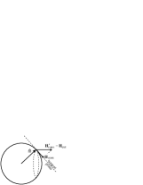
Figure 5: Magnetization vector for the simplest case of precession about a horizontal external field, showing the $\mathbf{M}$-sphere, the tangent plane (perpendicular to the paper) and the projected field $\mathbf{H}_{\text{cons}}$.  The dotted circle is the Stoner-Wohlfarth orbit, a curve of constant energy.

The directions of the various torques in the LL equation are shown in insets to Fig. 2 of the text,which also shows the contours of constant energy on a planar projection of the $\mathbf{M}$-sphere. For in-plane $\mathbf{M}$ ($\theta=\pi/2)$, the directions are particularly simple, as shown in the lower inset of Fig. 2  The conservative (precession) term $\dot{\mathbf{M}}_{\text{cons}}$ is vertical (along the energy contour, i.e., the Stoner-Wohlfarth orbit), the LL damping term $\dot{\mathbf{M}}_{\text{LL}}$ is horizontal (along the negative energy gradient, i.e., $\mathbf{H}_{\text{cons}}$), and the Slonczewski torque term is horizontal and opposite to the damping term (for our choice of sign for the current).

For a general direction of $\mathbf{M}$, (upper inset) the precession and LL damping torques are still exactly along and perpendicular to the orbit, respectively.  The Slonczewski torque $\dot{\mathbf{M}}_{\text{Slon}}$, on the other hand, can be in any direction, depending on the thick-layer magnetization direction.

A.4 Derivation of Fokker-Planck equation

Inserting Eq. 10 for the current $\mathbf{j}(\mathbf{M},t)$ into the continuity equation (9) gives the FP equation

$$\frac{\partial\rho}{\partial t}=D\nabla^{2}\rho-\nabla\cdot\mathbf{(\rho}\dot{\mathbf{M}}_{\text{det}})\text{.}$$ (26)

This is identical to the FP equation derived by Brownbrown , though the latter looks more complicated because the 2D Laplacian is written explicitly in spherical coordinates.  It is important that the divergence is two-dimensional here. If a three-dimensional divergence is used, it has been shown [J. L. Garcia-Palacios and F. J. Lazaro, ”Langevin dynamics study of the dynamical properties of small magnetic particles”, Phys. Rev. B 58, 14937 (1998)] that the Itô interpretation of the LL equation gives an extra (radial) term in the probability current J, relative to the Stratonovich interpretation. By working entirely in the spherical surface, we ensure that the Itô and Stratonovich results are the same.

A.5 Derivation of energy current

By definition of the 2D current $\mathbf{j}(\mathbf{M},t)$, the rate at which systems cross the length element $d\mathbf{M}$ (Fig. 6) along the contour (i.e., Stoner-Wohlfarth orbit) is the component of $\mathbf{j}$ perpendicular to the element.

Figure 6: A length element $d\mathbf{M}$ along an orbit, for derivation of the energy-current equation ((13)).  The plane of the figure is the tangent plane to the $\mathbf{M}$-sphere.

Thus the total rate of crossing from lower to higher $E$ is an integral over the orbit:

$$j^{E}_{i}(E,t)=\oint\left[\mathbf{j}(\mathbf{M},t)\times d\mathbf{M}\right]\cdot\hat{\mathbf{m}}$$ (27)

Using Eqs. 10 and 2 for $\mathbf{j}$, we obtain

$$j^{E}_{i}(E,t)=\oint\left[\rho(\mathbf{M},t)\dot{\mathbf{M}}_{\text{det}}(\mathbf{M})\right]\cdot\hat{\mathbf{m}}-\oint\left[D\nabla\rho(\mathbf{M},t)\times d\mathbf{M}\right]\cdot\hat{\mathbf{m}}$$ (28)

The current from the conservative term (Eq. 3) is along $d\mathbf{M}$ and does not contribute to $j^{E}_{i}$. The current (omitting the subscript $i$ since we deal with only one well) then has three terms:

$$j^{E}(E,t)=j^{E}_{\text{LL}}(E,t)+j^{E}_{\text{Slon}}(E,t)+j^{E}_{\text{diff}}(E,t)$$ (29)

The first (Landau-Lifshitz damping) term comes from the Landau-Lifshitz damping torque $\dot{\mathbf{M}}_{\text{LL}}$ (Eq. 6):

$$j_{\text{LL}}^{E}(E,t)=\gamma\alpha M_{s}\oint\left[\rho(\mathbf{M},t)\mathbf{H}_{\text{cons}}\times d\mathbf{M}\right]\cdot\hat{\mathbf{m}}=-\gamma\alpha M_{s}\rho^{\prime}(E,t)I_{i}^{E}(E)$$ (30)

where we have used the fact that the energy is constant over the orbit to bring $\rho$ (Eq. 11) out of the integral, and defined a (positive) energy integral $I_{i}^{E}$ by

$$I_{i}^{E}(E)\equiv\oint\left[d\mathbf{M}\times\mathbf{H}_{\text{cons}}\right]\cdot\hat{\mathbf{m}}=\oint H_{\text{cons}}dM$$ (31)

We obtain the last expression because the three vectors in the triple product are mutually orthogonal.

The remaining term in the deterministic torque is the Slonczewski torque

$$\dot{\mathbf{M}}_{\text{Slon}}=-\gamma JM_{s}\hat{\mathbf{m}}\times(\hat{\mathbf{m}}\times\hat{\mathbf{m}}_{\text{p}})=-\gamma JM_{s}\left[\hat{\mathbf{m}}(\hat{\mathbf{m}}\cdot\hat{\mathbf{m}}_{\text{p}})-\hat{\mathbf{m}}_{\text{p}}\right]$$ (32)

which gives an energy current

$$j_{\text{Slon}}^{E}(E,t)=-\gamma JM_{s}\oint\left[\rho(\mathbf{M},t)\left[\hat{\mathbf{m}}(\hat{\mathbf{m}}\cdot\hat{\mathbf{m}}_{\text{p}})-\hat{\mathbf{m}}_{\text{p}}\right]\times d\mathbf{M}\right]\cdot\hat{\mathbf{m}}=\gamma JM_{s}\hat{\rho^{\prime}(E,t)\mathbf{m}}_{\text{p}}\cdot\oint\left[d\mathbf{M}\times\hat{\mathbf{m}}\right]$$ (33)

since the first term in the cross product is orthogonal to $\hat{\mathbf{m}}$. Defining the magnetization integral

$$\mathbf{I}_{i}^{M}(E)=\oint d\mathbf{M}\times\mathbf{M}$$ (34)

gives

$$j_{\text{Slon}}^{E}(E,t)=\gamma J\hat{\rho^{\prime}(E,t)\mathbf{m}}_{\text{p}}\cdot\mathbf{I}_{i}^{M}$$ (35)

The last (diffusive) term in Eq. 28 involves

$$\nabla\rho(\mathbf{M},t)=\nabla\rho^{\prime}(E(\mathbf{M}),t)=\frac{\partial\rho^{\prime}(E,t)}{\partial E}\nabla E(\mathbf{M})=-\frac{\partial\rho^{\prime}(E,t)}{\partial E}\mathbf{H}_{\text{cons}}$$ (36)

and gives the same triple vector product as the Landau-Lifshitz damping term (Eq. 30):

$$j^{E}_{\text{diff}}(E,t)=D\frac{\partial\rho^{\prime}(E,t)}{\partial E}\oint\left[\mathbf{H}_{\text{cons}}\times d\mathbf{M}\right]\cdot\hat{\mathbf{m}}=-D\frac{\partial\rho^{\prime}(E,t)}{\partial E}I_{i}^{E}(E);$$ (37)

Our final result for the total energy current (Eq. 29) is thus Eq. 13.  Inserting this current into the continuity equation (Eq. 12) gives the energy Fokker-Planck equation.

Since Kramers used the FP equation in energy only in the low-damping limit, which might suggest that it is an approximation valid only in that limit, it is important to realize that it is not an approximation at all – as long as the probability density $\rho$ is constant along an orbit, it gives the exact evolution of $\rho(E,t)$.

In a steady state, the energy current (Eq. 13) vanishes, giving Eq. 16:

$$\frac{\partial\ln\rho^{\prime}(E)}{\partial E}=\frac{\gamma}{D}\left[-\alpha M_{s}+\eta(E)J\right]\equiv-V\beta(E)$$ (38)

This involves the ratio (Eq. 17)

$$\eta(E)=\frac{\hat{\mathbf{m}}_{\text{p}}\cdot\mathbf{I}_{i}^{M}(E)}{I_{i}^{E}(E)}.$$ (39)

plotted in Fig. 3. We have calculated the integrals by solving the LL equation numerically at each energy; an analytic check is possible at the bottom of each well (at the left end of the $\eta_{1}$ or $\eta_{2}$ curve), where $|\eta_{i}(E_{i})|=M_{s}/[\frac{1}{2}M_{s}+H_{K}\mp H_{\text{ext}}]\sim 2$.

A.6 Solving the FP equation in energy

We can write the inverse effective Maxwell-Boltzmann temperature defined by Eq. 38 or 16 as

$$\beta_{i}(E)=\frac{1}{k_{B}T_{MB}}=\frac{1}{k_{B}T}[1-\eta_{i}(E)J/\alpha M_{s}]$$ (40)

in terms of which Eq. 19 can be written

$$\rho_{i}^{\prime}(E)=\rho^{\prime}(E_{\text{sad}})\exp\left[V\int\limits_{E}^{E_{\text{sad}}}\beta_{i}(E^{\prime})dE^{\prime}\right]$$ (41)

Note that $\rho^{\prime}(E_{\text{sad}})$ has no region index because it is the same in all three regions. If $\beta_{i}(E)$ is independent of energy, Eq. 41 becomes the usual Maxwell-Boltzmann distribution; in any event it is easy to integrate numerically.

Current-driven thermal switching can be understood in terms of the increase in the Arrhenius rate due to this temperature increase.  If we increase the current $J$ enough, the temperature at the bottom of the well can be made negative; this can be used to model the onset of microwave noise, although our first-order treatment of $J$ will eventually fail and we will need to work in terms of nonzero-$J$ orbits rather than the present unperturbed orbits.

A.7 Derivation of TST (transition state theory) rate

The TST rate is the probability per unit time of crossing the dotted line in Fig. 7, which follows the energy gradient from the saddle point.

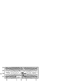
Figure 7: The contour plot of Fig. 2, showing the dashed line across which switching from region 2 to region 1 takes place, along which we integrate the current to obtain the total TST rate.

This is independent of the damping coefficient, since the damping current $\rho\dot{\mathbf{M}}_{\text{LL}}$ (Eq. 6) has no component normal to this line, nor does the diffusive current $-D\nabla\rho$, and the conservative and Slonczewski currents are independent of damping.  To lowest order in the electric current $J$, we need only include the conservative current, and the probability current (left to right) is given by an integral like Eq. 28:

$$j_{\text{TST}}=-\oint\left[\mathbf{j}_{\text{cons}}(\mathbf{M})\times d\mathbf{M}\right]\cdot\hat{\mathbf{m}}=-\oint\left[\dot{\rho\mathbf{M}}_{\text{cons}}\times d\mathbf{M}\right]\cdot\hat{\mathbf{m}}$$ (42)

[Since we are in a steady state, the reverse current (right to left, across a similar line pointing upward from the saddle point in Fig. 7) is equal in magnitude.] Using Eq. 3, and observing from Fig. 7 that all the cross products involve perpendicular vectors, we obtain

$$j_{\text{TST}}=\gamma M_{s}\oint\rho_{3}^{\prime}(E)H_{\text{cons}}dM=\frac{\gamma M_{s}}{\mu_{0}}\int_{E_{\text{sad}}}^{\infty}\rho_{3}^{\prime}(E)dE$$ (43)

where we have used $dE=\mu_{0}H_{\text{cons}}dM$ (Eq. 4).  The analog of Eq. 19 for the region $E>E_{\text{sad}}$ where we integrate up instead of down from $E_{\text{sad}}$) is

$$\rho_{3}^{\prime}(E)=\rho^{\prime}(E_{\text{sad}})\exp\left[-\frac{V}{k_{B}T}[1-\overline{\eta_{3}}(E)J/\alpha M_{s}][E-E_{\text{sad}}]\right]$$ (44)

so that

$$j_{\text{TST}}=\frac{\gamma M_{s}}{\mu_{0}}\rho^{\prime}(E_{\text{sad}})\int_{E_{\text{sad}}}^{\infty}\exp\left[-\frac{V}{k_{B}T}[1-\overline{\eta_{3}}(E)J/\alpha M_{s}][E-E_{\text{sad}}]\right]dE$$ (45)

Noting from Fig. 3 that $\overline{\eta_{3}}$ is slowly varying within $k_{B}T$ of $E_{\text{sad}}$, we approximate it by a constant so the integral is analytic:

$$j_{\text{TST}}=\frac{\gamma M_{s}k_{B}T}{\mu_{0}V[1-\overline{\eta_{3}}(E)J/\alpha M_{s}]}\rho^{\prime}(E_{\text{sad}})$$ (46)

It may seem inconsistent to include a term in $J/\alpha$ when we are working to lowest order in $J$; however, since $\alpha$ is also small, we really work to lowest order in both, and $J/\alpha$ is of zeroeth order in this sense.

In the chemical reaction rate literaturechandler it is found that TST gives a good representation of the switching rates as long as a trajectory that crosses the saddle point from the initial to the final well is likely to be trapped there by losing energy to LL damping.  The LL damping constants in magnetic materials are large enough (0.01-0.02) that escape after one orbit in the final well is quite unlikely, so the TST is likely to be quite accurate.  Our telegraph-noise fitting involves rates that vary by many orders of magnitude, so corrections to TST of a few percent are not critically important.

A.8 Derivation of dwell times

The total probability of being in well $i$ (= 1 or 2) is obtained by integrating the density over the well.  The probability of being in a surface element $d^{2}M$ on the M-sphere with energy $E$ is $\rho^{\prime}(E)d^{2}M$, so the probability of being in the ring shown in Fig. 8 is

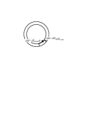
Figure 8: A ring on the M-sphere representing energies between $E$ and $E+dE$, showing the dimensions $dM$ and $dM^{\prime}$ of an area element.

$$\int\rho^{\prime}(E)\dot{\mathbf{M}}_{\text{cons}}dtdE/\mu_{0}H_{\text{cons}}=\gamma\rho^{\prime}(E)\int M_{s}H_{\text{cons}}dtdE/\mu_{0}H_{\text{cons}}=\frac{\gamma M_{s}P_{i}(E)}{\mu_{0}}\rho^{\prime}(E)dE$$ (47)

where $P_{i}(E)$ is the period of the orbit. Thus the well probability is (using Eq. 44 for $\rho_{3}^{\prime}$)

$$p_{i}=\int_{E_{i}}^{E_{\text{sad}}}\frac{\gamma M_{s}P_{i}(E)}{\mu_{0}}\rho_{i}^{\prime}(E)dE=\rho^{\prime}(E_{\text{sad}})\frac{\gamma M_{s}}{\mu_{0}}\int_{E_{i}}^{E_{\text{sad}}}P_{i}(E)\exp\left[\frac{V}{k_{B}T}[1-\overline{\eta_{i}}(E)J/\alpha M_{s}][E_{\text{sad}}-E]\right]dE$$ (48)

where $E_{i}$ is the energy at the bottom of well $i$.  Again, $\overline{\eta_{i}}(E)$ and $P_{i}(E)$ are nearly independent of $E$, which is true in the lowest few $k_{B}T$ of the well, so this integrates to

$$p_{i}=\frac{\gamma M_{s}P_{i}(E_{i})}{\mu_{0}V}\frac{\rho^{\prime}(E_{\text{sad}})k_{B}T}{1-\overline{\eta_{i}}(E_{i})J/\alpha M_{s}}\left[\exp\left[\frac{V}{k_{B}T}[1-\overline{\eta_{i}}(E_{i})J/\alpha M_{s}]E_{i}^{b}\right]-1\right]$$ (49)

Then the dwell time is

$$\tau_{i}=\frac{p_{i}}{j_{\text{TST}}}=P_{i}(E_{i})\frac{1-\overline{\eta_{3}}(E_{\text{sad}})J/\alpha M_{s}}{1-\overline{\eta_{i}}(E_{i})J/\alpha M_{s}}\left[\exp\left[\frac{V}{k_{B}T}[1-\overline{\eta_{i}}(E_{i})J/\alpha M_{s}]E_{i}^{b}\right]-1\right]$$ (50)

where $E_{i}^{b}\equiv E_{\text{sad}}-E_{i}$ is the barrier height.  The important thing to notice is that $\overline{\eta_{1}}$ and $\overline{\eta_{2}}$ have opposite signs, so one dwell time increases exponentially with $J$ and the other decreases, as in Fig. 4.

A.9 Determination of energy barriers

One virtue of the fitting scheme described in the text and illustrated in Fig. 4 is that we can determine the stability factor $S_{i}\equiv VE^{b}_{i}/k_{B}T_{i}$ of each well independently, where the barriers are given bybrown

$$E^{b}_{i}=(1\mp H_{\text{ext}}/H_{K})^{2}KV/k_{B}T_{i}$$ (51)

though these are in turn consistent with many choices of anisotropy $K=H_{K}M_{s}/2$, effective external field $H_{\text{ext}}$, temperature $T_{i}$ , and volume $V$.  For example, if we assume the wells are at the same temperature and $H_{\text{ext}}=-120$ Oe, we obtain

$$H_{K}=220\text{ Oe .}$$ (52)

If we further assume the experimental estimateurazhdin $V=3.67\times 10^{-23}$ m${}^{3},$ we obtain an effective temperature $T=730$ K. (Of course, this could be reduced to room temperature by assuming a smaller effective volume.)

References

- (1) F. J. Albert, J. A. Katine, R A. Buhrman, and D. C. Ralph, ”Spin-Polarized Current switching of a Co thin film nanomagnet”, Appl. Phys. Lett. 77, 3809 (2000).
- (2) E. B. Myers, F. J. Albert, J. C. Sankey, E. Bonet, R A. Buhrman, and D. C. Ralph, ”Thermally Activated Magnetic Reveral Induced by a Spin-Polarized Current”, Phys. Rev. Lett. 89, 196801 (2002).
- (3) Z. Li and S.Zhang, ”Magnetization dynamics with a spin-transfer torque”, Phys. Rev. B 68, 024404 (2003).
- (4) Z. Li and S.Zhang, ”Thermally assisted magnetization reversal in the presence of a spin-transfer torque”, cond-mat 0302339 (2003).
- (5) J. Slonczewski, ”Current-driven excitation of magnetic multilayers”, J. Magn. Magn. Mater. 159, L1 (1996).
- (6) J. Slonczewski, ”Excitation of spin waves by an electric current”,J. Magn. Magn. Mater. 195, L261 (1999).
- (7) S. Urazhdin, N.O. Birge, W.P. Pratt, and J. Bass, ”Current-Driven Magnetic Exciations in Permalloy-Based Multilayer Nanopillars”, Phys. Rev. Lett. 91, 146803 (2003).
- (8) J.-E. Wegrowe et al, ”Spin-polarized current induced magnetization switch: Is the modulus of the magnetic layer conserved?”, J. Appl. Phys. 91, 8606 (2002).
- (9) R. H. Koch, J. A. Katine, and J. Z. Sun, ”Time-resolved Reversal of Spin-Transfer Switching in a Nanomagnet”, Phys. Rev. Lett. 92, 088302 (2004).
- (10) H. A. Kramers, ”Brownian motion in a field of force and the diffusion model of chemical reactions”, Physica VII, 284 (1940).
- (11) H. Eyring, J. Chem. Phys. 3, 107 (1935).
- (12) D. Chandler, in “Classical and Quantum Dynamics in Condensed Phase Simulations”, ed. B. J. Berne, G. Ciccotti,and D. F. Coker, World Scientific, Singapore, 1998, p. 3.
- (13) P. B. Visscher, ”Numerical Brownian-motion Model Reaction Rates”, Phys. Rev. B 14, 347-353 (1976).
- (14) W. F. Brown, ”Thermal Fluctuations of a Single-Domain Particle”, Phys. Rev. 130, 1677 (1963).
- (15) W. T. Coffey et al, ”Thermally Activated Relaxation Time of a Single Domain Ferromagnetic Particle Subjected to a Uniform Field at an Oblique Angle to the Easy Axis: Comparison with Experimental Observations”, Phys. Rev. Lett. 80, 5655 (1998).
- (16) J. Fidler and T. Schrefl, J. Phys. D 33, R153 (2000).
- (17) EPAPS document E-xx-xxxxx. This EPAPS supplementary document contains some details of derivations for which there was not space in this Letter.
- (18) S. I. Kiselev, J. C. Sankey, I. N. Krivorotov, N. C. Emley, R. J. Schoelkopf, R. A. Buhrman, and D. C. Ralph, ”Microwave oscillations of a nanomagnet driven by a spin-polarized current”, Nature 425, 380 (2003).
- (19) J. G. Zhu and X. Zhu,”Spin transfer induced noise in CPP read heads”,submitted to Proceedings of TMRC, paper A2.