Competition of hydrophobic and Coulombic interactions between nano-sized solutes

Abstract

The solvation of charged, nanometer-sized spherical solutes in water, and the effective, solvent-induced force between two such solutes are investigated by constant temperature and pressure Molecular Dynamics simulations of model solutes carrying various charge patterns. The results for neutral solutes agree well with earlier findings, and with predictions of simple macroscopic considerations: substantial hydrophobic attraction may be traced back to strong depletion (“drying”) of the solvent between the solutes. This hydrophobic attraction is strongly reduced when the solutes are uniformly charged, and the total force becomes repulsive at sufficiently high charge; there is a significant asymmetry between anionic and cationic solute pairs, the latter experiencing a lesser hydrophobic attraction. The situation becomes more complex when the solutes carry discrete (rather than uniform) charge patterns. Due to antagonistic effects of the resulting hydrophilic and hydrophobic “patches” on the solvent molecules, water is once more significantly depleted around the solutes, and the effective interaction reverts to being mainly attractive, despite the direct electrostatic repulsion between solutes. Examination of a highly coarse-grained configurational probability density shows that the relative orientation of the two solutes is very different in explicit solvent, compared to the prediction of the crude implicit solvent representation. The present study strongly suggests that a realistic modeling of the charge distribution on the surface of globular proteins, as well as the molecular treatment of water are essential prerequisites for any reliable study of protein aggregation.

I Introduction

It is a well-known fact of physical chemistry that solvophobic solutes of similar sizes and shapes tend to attract each other in an incompatible solvent. Classic examples are the effective attraction between monomers of polymer coils in poor solvent, which leads to collapse below the $\Theta$-temperature,Rubinstein and Colby (2003) or the attraction between hydrophobic surfaces in water.Chandler (2004) The effective attraction ultimately leads to phase separation of the solvent and solute as the concentration of the latter increases. The solvent-averaged effective interaction (or potential of mean force) is related to the variation of free energy upon bringing the two solutes from infinite to a finite separation in the solvent. The change in free energy has an entropic component, associated with the reorganization of the solvent molecules around the two solutes, and an energetic contribution which accounts for the deficit in attractive interactions between solvent molecules close to the solutes. There is some analogy between solvophobic attraction and the well-known depletion interaction between colloidal particles induced by a depletant like non-adsorbing polymers.Likos (2001) In the latter case the depletion attraction can be essentially understood in terms of excluded volume, and is hence of entropic origin, while hydrophobic interactions have a large energetic contribution, associated with the formation or break up of hydrogen bonds.

It has been recognized that the size of the solute plays an important role in understanding its solvation energy, and effective solute-solute attraction.Chandler (2004) For solutes of a characteristic size larger than a few molecular diameters (typically larger than 1nm), a mechanism first envisioned by Stilinger Stilinger (1973) is that of solvent dewetting (“drying”), i.e. the solvent molecules tend to move away from the surface of a large solute, and form a liquid-gas like interface parallel to the solute interface.Chandler (2004); Hummer and Garde (1998) The overlap of the drying zones associated with two large solutes as their surfaces come together may then give rise to an effective attraction,Lum et al. (1999) very much like the depletion mechanism between-colloidal particles. The mechanism holds, a priori, for any solvent, provided that it is in a thermodynamic state close to liquid-vapor coexistence.Huang et al. (2001) The drying mechanism and resulting attraction between two plate-like solutes was confirmed by Molecular Dynamics (MD) simulation of Wallquist and Berne.Wallquist and Berne (1995) Similar simulations were carried out for two large spherical solutes in a Lennard-Jones solvent, and attractive solvation force profiles were determined.Kinoshita et al. (1996); Shinto et al. (1999); Qin and Fichthorn (2003)

However most nano-scale biomolecular solutes, like proteins, carry electric charges, which make them, at least partly, hydrophilic. The main objective of the present paper is to investigate the influence of solute-solute and solute-solvent electrostatic interactions on the effective, solvent-induced potential of mean force between two solutes. In order to make contact with earlier work on neutral hard-sphere solutes, we restrict the present investigation to spherical solutes of identical radii $R\lesssim 1$nm, but carrying various surface charge patterns. The two main questions which will be addressed are: a) how does the competition between hydrophobicity and electrostatics affect the total effective force between anionic and cationic solutes; b) is the total force sensitive to details of the charge patterns carried by the solutes? In particular are there significant differences between results obtained with continuous and discrete charge patterns of the solutes? Such differences were recently highlighted by a calculation of the second virial coefficient in an implicit solvent model of globular proteins, which does not, of course, allow for hydrophobic attraction.Allahyarov et al. (2002)

We have attempted to answer these questions by a series of constant pressure MD simulations of two spherical solutes of varying radii (up to $R=1.3$nm) immersed in water modeled by the SPC/E intermolecular potential,Berendsen et al. (1987) taken under normal conditions, i.e. close to liquid-vapor coexistence. The paper is structured as follows. The models and simulation procedures are detailed in Sec. II. The solvation of single charged solutes is examined in Sec. III. The effective interaction between two solutes as a function of the mutual distance is estimated from a simple macroscopic theory in Sec. IV, where the method for extracting the mean effective force from simulations is also defined. The results from MD simulations for several charge patterns are presented in Sec. V, while concluding remarks are made in Sec. VI.

Part of the present results were briefly reported elsewhere.Dzubiella and Hansen (2003)

II Models and methodology

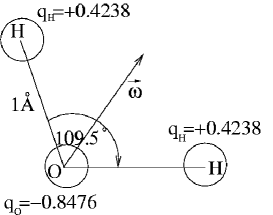
Figure 1: Sketch of the SPC/E water model. The vector $\vec{\omega}$ embodies the orientation of the molecule.

The MD simulations were carried out on periodic samples containing $N_{\rm w}$ water molecules and one or two solutes. The SPC/E model of a water molecule Berendsen et al. (1987) is sketched in Fig. 1. Two water molecules interact via a Lennard-Jones potential between the oxygen (O) sites, and the bare Coulomb potentials between the 9 pairs of sites. The Lennard-Jones parameters are $\epsilon=0.6502$kJmol^-1 and $\sigma=3.169$Å. The molecules are assumed to be rigid (with OH bond lengths and HOH bond angle specified in Fig. 1) and nonpolarizable. The solutes are smooth spheres of bare radius $R_{0}$, which interact with the O-site of the water molecules by the purely repulsive potential

$$V_{0}(r)=\phi(r-R_{0})^{-12},$$ (1)

where $r$ is the distance from the solute center to the O-site, and the energy scale $\phi$ is chosen such that the O-atom experiences a repulsive energy $k_{\rm B}T$ at a distance $r-R_{0}=$1Å  from the solute surface. With this convention, the effective radius of the solutes may be defined as $R=R_{0}+1$Å. The purely repulsive interaction (1) is chosen to mimic a strongly hydrophobic interaction between the neutral solute and the water molecules. The model involving spherical solutes with no charged site will be referred to as ${\rm S}_{0}$.

Since the main objective of our work is to investigate the difference in the effective, solvent induced interaction between the cases of neutral and charged solutes, we have considered several models for the latter (cf. Table 1). In the simplest model, a total charge $Q=qe$ (where $e$ is the proton charge) is assumed to be uniformly distributed over the solute surface. According to Gauss’ theorem, this is equivalent to placing a single charged site $Q$ at the center of the spherical solute. We consider both anionic ($q<0$) and cationic ($q>0$) solutes and the corresponding models will be referred to as ${\rm S}_{-}$ and ${\rm S}_{+}$. To ensure overall electroneutrality of the system, the total charge carried by the solutes must be compensated either by a uniform background of total opposite charge permeating the system, or by explicitly including counterions. For the latter we choose Cl^- (cationic solutes) and Na⁺ (anionic solutes) ions. Their mutual interactions and coupling to water molecules involve the standard Coulomb-interactions, and a Lennard-Jones part, with $\epsilon$ and $\sigma$ parameters taken from Spohr.Spohr (1999) The short range interaction with the solutes is again described by (1).

	${\rm S}_{0}$	${\rm S}_{+}$	${\rm S}_{-}$	${\rm T}_{0}$	${\rm T}_{+}$	${\rm T}_{-}$	${\rm C}_{0}$	${\rm C}_{+}$	${\rm C}_{-}$
$N_{c}$	0	1	1	4	4	4	8	8	8
$Q/e$	0	q	-q	0	4	-4	0	8	-8
$R_{0}/{\rm\AA}$	$0-12$	10	10	10	10	10	10	10	10
$R_{c}/{\rm\AA}$	-	0	0	10	10	10	10	10	10
$R_{cc}/{\rm\AA}$	-	0	0	16.33	16.33	16.33	11.55	11.55	11.55

Table 1: Characteristics of the different models ${\rm S}_{0\pm},{\rm T}_{0\pm},{\rm C}_{0\pm}$ used. $N_{c}$ is the number of charges carried by the solute, while $Q$ is the net charge. $R_{0}$ is the bare solute radius. By $R_{c}$ we denote the distance of the charges to the center of the solute, and $R_{cc}$ quantifies the nearest neighbor distance between the charges. In the charged ${\rm S}$-models the charge is located in the center of the solutes, while in the ${\rm T}$ and ${\rm C}$ models the charges are distributed tetrahedrally and cubically on the sphere surface.

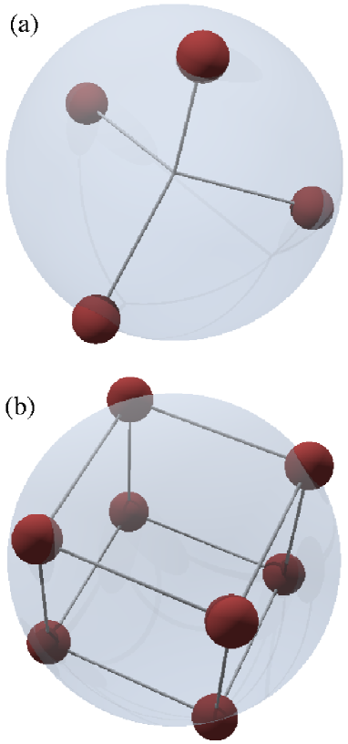
Figure 2: Solute with (a) tetrahedral (T models) and (b) cubic (C models) charge distribution. The charges are connected in this figure for a better visualization of the structure.

In order to investigate the sensitivity of the effective forces to details of the solute charge patterns, we have also considered models with discrete charge distributions involving $N_{c}$ point charges placed on the surface of the solutes. In the tetrahedron model, $N_{c}=4$ charges are tetrahedrally arranged at a distance $R_{0}$ from the center of the solutes, as illustrated in Fig. 2(a); we consider both the cases where all 4 charges are of the same sign ($q=\pm 4$, referred to as models ${\rm T}_{+}$ and ${\rm T}_{-}$), and the neutral situation, where two charges are positive and two are negative (model ${\rm T}_{0}$). We have also considered cubic charge distributions, as sketched in Fig. 2(b), where $N_{c}=8$. In models ${\rm C}_{+}$ and ${\rm C}_{-}$ all 8 charges are positive ($q=8$) or negative ($q=-8$), whereas in model ${\rm C}_{0}$, four vertices carry a charge $+e$, while the other four carry opposite charges in an alternating arrangement such that the three nearest neighbors of a negative charge are positive and vice versa. A similar model of globular proteins was considered by Allahyarov et al.,Allahyarov et al. (2002) but in an implicit (continuous) solvent representation.

In order to avoid very close approaches of water H-sites and the solute surface charges, the charged sites at the vertices of the tetrahedron or cube, situated at a distance $R_{0}$ from the solute center, are not simply point charges, but are modeled by Cl^- or Na⁺ ions. The corresponding LJ potentials prevent these sites and the water H atoms to come too close, and hence unreasonably large electrostatic forces, which could lead to electrostatic “sticking” of the water molecules to the solute surface. The total interaction energy between one solute and the $N_{\rm w}$ water molecules in a periodically repeated, cubic simulation cell is:

$$V_{\rm sol} = \sum_{i=1}^{N_{\rm w}}V_{\rm 0}(r_{i})+\sum_{i=1}^{N_{w}}\sum_{\alpha=1}^{N_{\rm c}}V_{\rm LJ}(r_{i}^{\alpha 1})$$ (2)

$$+ \sum_{i=1}^{N_{w}}\sum_{\alpha=1}^{N_{\rm c}}\sum_{\beta=1}^{3}{q_{\alpha}}{q_{\beta}}\phi_{\rm EW}(\vec{r}_{i}^{\alpha\beta}),$$

where $r_{i}$ is the distance from the center of the solute to the O-atom of the $i$th water molecule, and $r_{i}^{\alpha\beta}$ is the distance from site $\alpha$ on the solute to site $\beta$ of the $i$th water molecule ($\beta=1$ for the oxygen site). The first term on the rhs of Eq. (2) corresponds to the short ranged repulsion (1); the second term is the sum of Lennard-Jones interactions between all $N_{c}$ sites of the solute and the O-sites ($\beta=1$) of the $N_{\rm w}$ water molecules, which depend on the corresponding site-site distance $r_{i}^{\alpha 1}$; finally the last term accounts for the Coulombic interactions between all $N_{c}$ solute sites and all 3 water sites; $\phi_{\rm EW}(\vec{r})$ is the electrostatic interaction between two elementary charges, properly summed over an infinite array of periodic images, using the smooth-particle-mesh Ewald (SPME) method Essmann et al. (1995) (see the Appendix A for details). An expression similar to Eq. (2) holds for the total interaction between a solute and its Cl^- or Na⁺ counterions.

The MD simulations were carried out with the DLPOLY2 Smith and Forester (1999) package, using the Verlet leapfrog algorithm,Frenkel and Smit (1996) with a timestep of 2fs. Simulations were carried out at constant pressure ($P=1$atm) and constant temperature ($T=300$K), using appropriate barostats and thermostats (see Appendix A). We emphasize the importance of using constant pressure simulations of charged, aqueous systems: electrostriction and drying mechanisms modify the density of water in a finite, closed system in a significant way. In the present $NPT$ ensemble simulations, the overall density of water varied from $\rho_{0}=0.033{\rm\AA}^{-3}$ to $0.035{\rm\AA}^{-3}$; in estimating the average water density, the effective volume $4\pi R^{3}/3$ of the solutes must be subtracted. The choice of the box length $L$ of the periodically repeated simulation cell and the arrangement of solutes inside the cell are discussed in the Appendix A. The cell contained up to $N_{\rm w}=3000$ water molecules.

III Solvation of a single charged solute

Before embarking on the main subject of this paper, namely the water-induced effective interaction between two protein-like solutes, we first consider the solvation of a single, neutral or charged spherical solute, a problem which has been abundantly addressed in the literature, since the pioneering work of Born Born (1920) on solvation free energies of ions, and of Reiss et al. on the scaled-particle theory of cavity formation and hard sphere solutes. Reiss et al. (1959)

III.1 Water structure around a solute

Consider first the structure of water around an isolated neutral solute (model ${\rm S}_{0}$). Fig. 3 shows MD results for the oxygen and hydrogen radial distribution functions (RDF), or density profiles, around a solute for various solute radii $R$. The height of the main peak in the RDF of both O and H sites of the water molecules is seen to first grow with increasing $R$, and this may be rationalized in terms of enhanced packing of the molecules at the surface of the solute. But for $R\gtrsim 5$Å, the peak height is seen to decrease monotonically, due to the unbalanced attraction experienced by the water molecules near the surface from bulk water. Very similar predictions of the depletion of water around large spherical solutes (or cavities) have been reported earlier in the literature.Stilinger (1973); Huang et al. (2001); Lum et al. (1999) The hydrogen and oxygen peaks are located at nearly the same distance from the solute for any given radius $R$, with a tendency of the hydrogen peak to be slightly further out. This seems to indicate that there is no strong orientation of the water molecules in the first solvation shell towards or away from the solute surface.

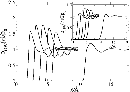
Figure 3: Density profiles of water oxygen and hydrogen atoms (inset) around one isolated neutral solute (${\rm S}_{0}$) plotted for different radii $R/{\rm\AA}=2,3,4,5,6,11$.

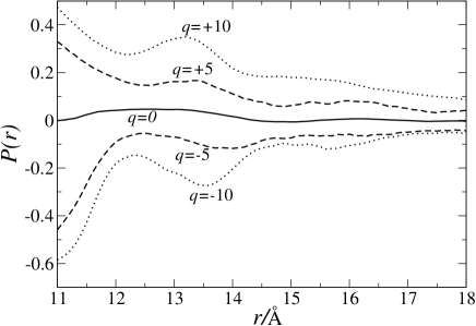
Figure 4: Orientation parameter $P(r)$ defined in Eq. (3) of the water particles around a solute with radius $R=11$Å  carrying no charge (${\rm S}_{0}$, solid line), and charge $q=\pm 5$ (${\rm S}_{\pm}$, dashed lines), and $q=\pm 10$ (${\rm S}_{\pm}$, dotted lines).

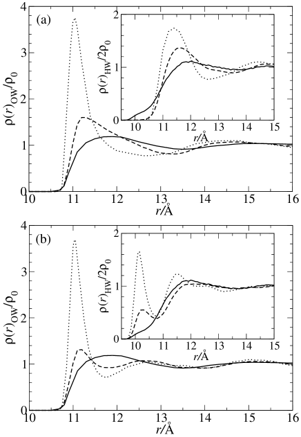
Figure 5: Density profiles of water oxygen and hydrogen atoms (inset) around a (a) positively (${\rm S}_{+}$) and (b) negatively (${\rm S}_{-}$) charged solute with radius $R=11$Å  and central charge $q=\pm 5$ (dashed line), and $q=\pm 10$ (dotted line). We also plot the result for the ${\rm S}_{0}$ model (solid line) with the same radius.

This observation may be quantified by considering the following orientational order parameter:

$$P(r)=\left<\frac{\vec{\omega}\cdot\vec{r}}{|\vec{\omega}||\vec{r}|}\right>_{r},$$ (3)

where $\vec{\omega}$ is the water molecule orientation vector (cf. Fig. 1), and the configurational average is taken for a fixed distance $r$ from the solute center to the O-site of the water molecules. MD results for a neutral solute of radius $R=11$Å  are plotted in Fig. 4. The curve $P(r)$ takes slightly positive values ($P\simeq 0.05$) for water in the first solvation shell ($r\simeq 12.5$Å), indicating a weak tendency of the hydrogen atoms to point away from the solute.

The effect of charging the solute is illustrated in Fig. 5(a) and (b), where the RDFs are plotted for a fixed radius $R=11$Å, and charges $q=0,\pm 5$, and $\pm 10$, within the ${\rm S}_{0}$ and ${\rm S}_{\pm}$ models (neutral, or uniformly charged solutes). For positive charges, Fig. 5(a), the height of the first peak in both oxygen and hydrogen RDFs is seen to shift to shorter distances, and to increase as $q$ increases, signaling an effective attraction of the dipolar solvent molecules due to the radial electric field. The trend is similar for negative charges, as regards the oxygen RDF. However the initial first peak (at $r\simeq 12$Å  for $q=0$) in the hydrogen RDF is seen to split into a prepeak around $r\simeq 10$Å  and a broad feature close to the initial peak when $q=-5$. This points to a reorientation of the water molecules in the first hydration shell, with the positive hydrogen atom preferring being closer to the surface of the anionic solute. Further decrease of the negative charge $(q=-10)$ consolidates this structure, with two hydrogen peaks growing in amplitude (cf. Fig. 5(b)). Interestingly, while the hydrogen RDFs are very sensitive to the sign of the solute charge (${\rm S}_{+}$ versus ${\rm S}_{-}$), the amplitudes of the first peaks of the oxygen RDFs are nearly independent of this sign, but the peak around the positive solute appears to be broader, signaling a larger water coordination number in the first solvation shell. The corresponding orientational order parameter $P(r)$ is plotted in Fig. 4. The absolute value of $P(r)$ has maxima at contact $r\simeq 11$Å  and approximately one water diameter further away ($r\simeq 13.5$Å), and increases with absolute charge, irrespective of the sign of the charge carried by the solute. Closer inspection of the curves in Fig. 4 reveals, however, a significant asymmetry, if not in the overall shape of $P(r)$, at least in the amplitudes, which are typically $20\%$ larger for the negative solute. Anion/cation hydration asymmetry had already been reported for microscopic ions in aqueous solution.Latimer et al. (1939)

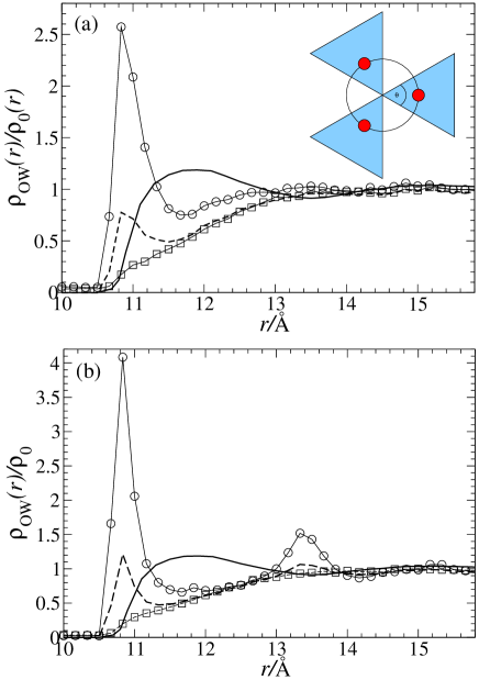
Figure 6: Oxygen density profiles around the tetrahedral (a) positive ${\rm T}_{+}$ and (b) negative ${\rm T}_{-}$ solutes. The curves are for a full angular average (long dashed lines), cone averages around the charges (circles), and averages of water excluded by these cones (squares), as explained in section III.1. We also plot the density profile around a neutral solute ${\rm S}_{0}$ (solid line) for comparison. The inset in (a) sketches a two dimensional projection of a tetrahedral solute. The cone averages are performed over the water molecules in the grey cones (opening angle $\Theta=30^{\circ}$) containing a surface charge (dark circle).

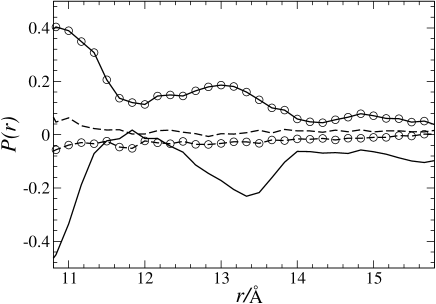
Figure 7: Orientation profiles $P(r)$ around the tetrahedral positive ${\rm T}_{+}$ (circles) and negative ${\rm T}_{-}$ (no symbols) solutes. Cone averages around charges (solid lines) are compared to averages of water molecules excluded by those cones (long dashed lines).

We now turn to the structure of water around a solute with an inhomogeneous charge distribution, restricting the discussion to the tetrahedral ${\rm T}_{+}$ and ${\rm T}_{-}$ models. In order to characterize the anisotropy of the problem, it is desirable to distinguish between water molecules close to the four surface charges, and the remaining water surrounding the solute. We achieve this by averaging over water molecules whose centers fall either inside or outside well-defined cones whose axes coincide with the radii joining the solute center and the surface charges and whose vertices coincide with the solute center. A sketch of the two-dimensional projection of one of the sides of the tetrahedron and its associated cones is shown in the inset to Fig. 6(a). Averages are taken over cones of opening angle $\Theta=30^{\circ}$, high enough to accommodate the first two solvation shells around a surface charge. The results for the oxygen density profiles for water molecules inside or outside the cones are shown in Figs. 6(a) and (b) for the ${\rm T}_{+}$ and ${\rm T}_{-}$ models, respectively. The water molecules inside the cones exhibit a typical solvation shell structure with a large first peak, and a much lower second peak, which is hardly visible in the ${\rm T}_{+}$ case. Outside the four cones, water appears to be highly depleted compared to its distribution around a neutral ${\rm S}_{0}$ solute, up to a radial distance $r\simeq 13$Å. Thus the 25$\%$ of the solute surface area inside the cones act as hydrophilic “patches” while the remaining 75% are hydrophobic. Interestingly, if an angular average is taken over the total solute area, the mean density of water close to the surface ($\lesssim 13$Å) of a ${\rm T}_{+}$ or ${\rm T}_{-}$ solute is significantly smaller than the corresponding density around a neutral ${\rm S}_{0}$ solute ! Integration of the water density profile up to $r=13$Å  yields coordination numbers (numbers of water molecules) of 133 for ${\rm S}_{0}$, 92 for ${\rm T}_{+}$, and 95 for ${\rm T}_{-}$, showing a 30$\%$ depletion of water around the T-solutes compared to ${\rm S}_{0}$. The orientational order parameter (3) for the ${\rm T}_{+}$ and ${\rm T}_{-}$ models are plotted versus $r$ in Fig 7. The orientational order of water molecules inside the cones is seen to be similar to that around homogeneously charged solutes ${\rm S}_{+}$ or ${\rm S}_{-}$ (cf. Fig. 4). In the depleted volumes outside the cones the water molecules shows little orientational order; if anything they tend to orient in the direction opposite to the mean orientation inside the cones.

Qualitatively similar observations hold for the distribution of water molecules around solutes with cubic charge distribution (models ${\rm C}_{+}$ or ${\rm C}_{-}$), but obviously the volumes depleted of water are now smaller, since the “hydrophobic patches” have shrunk now to only half of the solute surface area. The MD simulations for the solutes with non-vanishing net charge were carried out with explicit counterions. Test runs where these counterions were replaced by a uniform neutralizing background showed no differences within the statistical uncertainties.

III.2 Solvation free energy

The solvation free energy is equal to the reversible work required for transferring a solute from vacuum into a solvent. For neutral solutes in water, the solvation free energy is generally positive,Hummer et al. (1996); Lum et al. (1999) and for atomic-size solutes, it stems mainly from the entropy cost of the restructuring water molecules around the solute. For larger spherical solutes, a cross over in the variation of the solvation free energy with radius occurs typically around 1 nm.Lum et al. (1999) The classic Born model Born (1920) provides the simplest approach to the solvation free energy of charged spherical solutes. The solvent is treated as a dielectric continuum of permittivity $\epsilon$ and the hydration free energy increases quadratically with solute charge and is proportional to the inverse of the Born radius $R_{\rm B}$, according to

$$\Delta\mu_{\rm B}=-\frac{q^{2}e^{2}}{8\pi\epsilon_{0}R_{\rm B}}(1-1/\epsilon).$$ (4)

Note that the solvation free energy is a difference in chemical potential of the solute as it is moved from vacuum into the solvent. Hydration free energies from the Born model agree well with experimental values, once the unknown parameter $R_{\rm B}$ is defined. The Born radius for an ion can deviate substantially from its Pauling radius (a measure of the size of an ion).Latimer et al. (1939)

We have obtained solvation free energies for our model solutes by thermodynamic integration, using the general formula

$$\Delta\mu_{\rm sim}=\int_{\lambda_{0}}^{\lambda_{1}}d\lambda\left<\frac{\partial V_{\rm sol}}{\partial\lambda}\right>_{\lambda},$$ (5)

where the coupling parameter $\lambda$ gradually “switches on” the interaction (2) between the solute and the solvent from an initial state $\lambda=\lambda_{0}$ (say a neutral point solute) to a final state $\lambda=\lambda_{1}$ corresponding to the complete solute/solvent system. The brackets $<..>_{\lambda}$ denote a statistical average over all solute-solvent configurations for a solute-solvent coupling characterized by $V_{\rm sol}(\lambda)$. The index sim in $\Delta\mu_{\rm sim}$ indicates that the estimate of the solvation free energy is based on MD simulations of a finite sample; finite size corrections will be added as explained later.

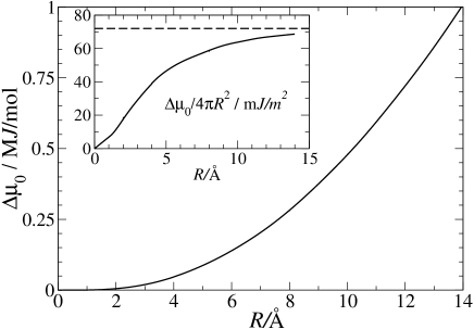
Figure 8: Solvation free energy $\Delta\mu_{0}$ of a neutral spherical solute ${\rm S}_{0}$ in water. The inset shows $\Delta\mu_{0}$ divided by the sphere surface showing an asymptotic approach for large $R$ to the liquid-vapor surface tension of water (dashed line), $\gamma\approx 72$mJ/${\rm m^{2}}$.

In practice, we proceded in two steps. In a first stage, we computed the solvation free energy $\Delta\mu_{0}$ of a neutral spherical solute (model ${\rm S}_{0}$), as a function of its radius $R$. The second step is to charge up the initially neutral solute to the final charge pattern. In step one, the coupling parameter $\lambda$ in Eq. (5) is simply the radius itself, and $\Delta\mu_{0}$ is consequently the work required to blow up the solute against the normal force exerted by the solvent, integrated over the particle surface; in this case the force is just the radial derivative of the first term on the rhs of eq (2). This is implemented, in practice, by starting from $\lambda_{0}=R=0$, and increasing the radius by steps of $\Delta\lambda=\Delta R=1$Å, up to $\lambda_{1}=14$Å  (the largest neutral solute considered in the present work). The averaged radial force, as obtained from the MD simulations for various $R$, is interpolated with a cubic spline and integrated to yield $\Delta\mu_{0}$. The resulting solvation free energy is plotted in Fig. 8, and is seen to increase monotonically with $R$. The solvation free energy per unit area, $\Delta\mu_{0}/4\pi R^{2}$, is plotted in the inset to Fig. 8, and is seen to approach asymptotically a constant value for radii $R\gtrsim 10$Å; the latter is close to the liquid-vapor surface tension of water, $\gamma=72$mJ/m². This behavior is close to that reported by Lum et al.Lum et al. (1999) for hard sphere cavities in water. The “softer” solute-solvent pair potential (1) used in the present work does not modify the solvation process significantly, compared to the case of hard sphere solutes.

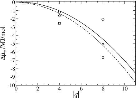
Figure 9: Excess solvation free energy $\Delta\mu_{\pm}$ of charging a spherical solute of radius $R=11$Å  in water homogeneously to a charge $q$ (solid line) and $-q$ (long dashed line). The symbols denote the solvation free energies of charging the ${\rm T}_{0\pm}$ and ${\rm C}_{0\pm}$ models in water. The symbols at $q=4$ are for the tetrahedron, at $q=8$ for the cube. The overall charge of the ${\rm T}_{0\pm}$ and ${\rm C}_{0\pm}$ solutes is zero (circles), positive (diamonds), and negative (squares).

In the second stage, to go from the neutral to the charged solute, the charges of the $N_{c}$ sites on the solute are gradually turned on, i.e. $q_{\alpha}(\lambda)=\lambda q_{\alpha}$ $(1\leq\alpha\leq N_{c})$, where $\lambda$ is varied from 0 to 1. The quantity to be averaged in Eq. (5) is now the total electrostatic energy of the solute in the field of the water molecules and their periodic images; the statistical average is to be taken over all Boltzmann-weighted water configurations when the electrostatic solute/solvent coupling is multiplied by $\lambda$. Since for any $\lambda>0$ the system carries a net charge, a compensating uniform background charge must be included in evaluating the Coulombic part of Eq. (2) by Ewald summation. If the self interaction energy of the solute with its own images and the neutralizing background is properly included, the resulting free energies are virtually independent of the size $L$ of the simulation box,Hummer et al. (1996, 1997) see the Appendix B. Results for $\Delta\mu_{\pm}$ corresponding to a uniformly charged solute with radius $R=11$Å  are plotted in Fig. 9 as a function of $q$, for anionic and cationic solutes. Note that this is the excess free energy for charging an initially neutral solute of $R=11$Å, previously inserted into the solvent, to a charge $q$. In order to obtain the total solvation free energy, the contribution $\Delta\mu_{0}$ corresponding to the insertion of the neutral solute in water ($\approx 0.6$MJ/mol for $R=11$Å) must be added to $\Delta\mu_{\pm}$. The curves are essentially quadratic on the scale shown, in agreement with Born theory. Least squares fits of the data to the Born formula (4) yield $R_{\rm B}^{+}=9.8$Å  and $R_{\rm B}^{-}=8.6$Å , both smaller than the effective solute radius $R=11$Å. The solvation free energy of cationic solutes is slightly positive for $0<q\lesssim 1$. Such a behavior has already been reported for small cationic solutes (e.g Na⁺)Hummer et al. (1996); Lynden-Bell and Rasaiah (1997) and may be understood from the competition between the free energy cost of the rearrangement of water around the solute, and the electrostatic energy gain of the dipolar solvent in the electric field of the solute. The latter contribution appears to dominate already for small $|q|$ in the case of anionic solutes, for which $\Delta\mu_{-}$ is always negative. Over the whole range of absolute charge $|q|$, $\Delta\mu_{-}$ is systematically lower than $\Delta\mu_{+}$, pointing to a preferential solvation of anionic solutes, again in agreement with earlier findings for other charged solute models.Hummer et al. (1996); Lynden-Bell and Rasaiah (1997); Rajamani et al. (2004) In Sec. III.1 we learned that the restructuring of water is stronger around an ${\rm S}_{-}$ solute than around its ${\rm S}_{+}$ counterpart, so that one would expect a higher cost in entropy. Apparently the closer approach of the hydrogen atoms to the negative solute decreases the electrostatic contribution to the free energy more than the positive entropic cost, resulting in an overall lower solvation free energy.

Solvation free energies for solutes carrying discrete tetrahedral or cubic charge distributions, corresponding to models ${\rm T}_{+}$, ${\rm T}_{-}$, and ${\rm T}_{0}$, and ${\rm C}_{+}$, ${\rm C}_{-}$, and ${\rm C}_{0}$ are also shown in Fig. 9. The contribution to the solvation free energy from the steric LJ-part of the surface charge interaction with the water molecules is insignificant and was neglected in the calculation of $\Delta\mu_{\pm}$. As in the case of the uniformly charged solutes, the negative solutes are preferentially solvated compared to their positive counterparts. The solvation energies of the overall neutral solutes ${\rm T}_{0}$ and ${\rm C}_{0}$ lie well above those of the charged solutes (${\rm T}_{\pm}$ or ${\rm C}_{\pm}$). In particular $|\Delta\mu|$ of the overall neutral solute with a cubic charge pattern ${\rm C}_{0}$ is roughly three times smaller than the corresponding $|\Delta\mu_{\pm}|$ of the globally charged solutes ${\rm C}_{+}$ and ${\rm C}_{-}$. This may be a consequence of the considerable reorganization of water around the solutes with surface charges of alternating sign, resulting in a substantial cost in free energy. Finally, the solvation free energies of solutes with discrete charge patterns (${\rm T}_{\pm}$ or ${\rm C}_{\pm}$) are seen to lie 10-20$\%$ below the solvation free energies of their uniformly charged counterparts ($S_{\pm}$ with $q=\pm 4$ and $\pm 8$).

IV Effective interaction between two solutes

We now turn to the main objective of this paper, namely the determination of the effective, solvent-mediated interaction between two nanometer-sized neutral or charged solutes in water. In subsection IV A and IV B we derive this interaction from simple macroscopic considerations, while the MD methodology is presented in IV C.

IV.1 Phenomenological theory for charged plates

A simple macroscopic argument, similar to Kelvin’s theory of capillary condensation predicts that water near liquid/vapor coexistence will undergo “drying” when confined between two hydrophilic plates, below a critical distance $D_{c}$ separating these plates.Lum et al. (1999) We extended the argument to the case of charged plates,Dzubiella and Hansen (2003) showing that $D_{c}$ is strongly reduced by the electrostatic energy associated with the surface charge carried by the plates. The macroscopic argument is further refined hereafter. Consider two parallel plate-like solutes of area $A_{1}$, separated by a distance $D$ and carrying opposite surface charges $\pm\sigma$, immersed in a polar solvent of dielectric permittivity $\epsilon$. Neglecting edge effects (an approximation valid as long as $D\ll A_{1}^{1/2}$, the electric field between the plates is $E_{0}/\epsilon$ with $E_{0}=\sigma/\epsilon_{0}$. We require the difference in the grand potential between the situations where the liquid solvent ($l$) or its vapor ($g$) fill the volume $A_{1}D$ between the two plates:

$$\Omega_{\alpha}=-P_{\alpha}A_{1}D+\frac{1}{2}\epsilon_{0}\frac{E^{2}_{0}}{\epsilon_{\alpha}}A_{1}D+2\gamma_{w\alpha}A_{1}+\gamma_{l\alpha}A_{2},$$ (6)

where $P_{\alpha}$ is the pressure of phase $\alpha=l,g$ and $\gamma_{w\alpha}$ the surface tension between phase $\alpha$ and the plate (“wall”). $A_{2}$ is the area of the liquid-vapor interface limited by the edges of the two opposite plates, which is created when the volume between the plates is filled by vapor. $\gamma_{l\alpha}$ is the liquid-vapor surface tension when $\alpha=g$, and vanishes of course when $\alpha=l$. The last term in Eq. (6) may be neglected for infinitely large plates.Dzubiella and Hansen (2003) Consider a state close to phase coexistence at temperature $T$, and let $\delta\mu=\mu-\mu_{\rm sat}$ be the positive deviation of the chemical potential from its saturation value. Expanding the $P_{\alpha}$ to linear order around their common value at saturation, one arrives at the following expression for the difference in grand potentials:

$$\Omega_{g}-\Omega_{l} = (\rho_{l}-\rho_{g})\delta\mu A_{1}D+\frac{\epsilon_{0}}{2}E^{2}_{0}(\frac{1}{\epsilon_{g}}-\frac{1}{\epsilon_{l}})A_{1}D$$ (7)

$$+ 2(\gamma_{wg}-\gamma_{wl})A_{1}-\gamma_{lg}A_{2}.$$

In water $\epsilon_{l}\equiv\epsilon\gg\epsilon_{g}\simeq 1$, $\rho_{g}\ll\rho_{l}$ (except near critical conditions) and $\gamma_{wl}-\gamma_{wg}=\gamma_{lg}\equiv\gamma$ for a purely hydrophobic surface. Moreover $A_{2}=UD$, where $U$ is the circumference of one plate. Hence:

$$\Delta\Omega=\left(\rho_{l}\delta\mu+\frac{\epsilon_{0}}{2}E^{2}_{0}\right)A_{1}D-2\gamma A_{1}+\gamma UD.$$ (8)

$\Delta\Omega=\Omega_{g}-\Omega_{l}$ is the reversible work bringing the two plates from infinite separation (when the volume between them is filled by liquid) to a distance $D$, at which “drying” has already occurred. At contact, $\Delta\Omega(D=0)=-2\gamma A_{1}$, and $\Delta\Omega$ increases linearly with $D$. The range of the purely attractive potential is defined by the distance $D_{c}$ at which $\Delta\Omega=0$; for $D>D_{c}$, the liquid is the preferred phase between the plates; for $D<D_{c}$, “drying” occurs. From Eq. (8) we obtain

$$D_{\rm c}\simeq\frac{2\gamma}{\rho_{l}\delta\mu+\frac{\epsilon_{0}}{2}E^{2}_{0}+\gamma U/A_{1}}.$$ (9)

Near the liquid-vapor transition of water $\delta\mu\ll k_{B}T$, and may be neglected compared to the surface tension term in the denominator. Consider circular plates of radius $R$; then $U/A_{1}=2R$, and if they are uncharged ($E_{0}=0$), $D_{c}=R$, which is in agreemeent with previous calculations of the mean force between plate-like solutes in water Wallquist and Berne (1995) and in a LJ-fluid.Bolhuis and Chandler (2000) In the case of high surface charges ($\sigma\lesssim e/{\rm nm}^{2}$), $E_{0}$ can be as large as $10^{10}$V/m, and the corresponding electrostatic term in the denominator becomes comparable to the surface term for solute sizes of a few nm. This leads to a strong reduction of $D_{\rm c}$ compared to the case of neutral solutes. This reduction of $D_{\rm c}$ hints at a considerable weakening of the hydrophobic interaction between two solutes when the latter are charged. This trend will be confirmed by the MD results in Sec. V. Note however that the simple macroscopic model ignores molecular details, and that its prediction does not, a priori, apply to solutes carrying discrete charge patterns (i.e. “hydrophilic patches”) for which a more microscopic description is required.

IV.2 Phenomenological theory for spherical solutes

The previous model can be extended to the case of neutral or charged spherical solutes with radius $R_{0}$ as follows (see Fig. 10). When “drying” occurs, the simulation data (cf. Fig. 13 (b) or (c)) suggest that a cylindrically symmetric domain bounded by the two spherical solute surfaces ($S_{1}$) and the curved liquid-vapor meniscus ($S_{2}$) is filled with vapor. The surface $S_{2}$ is assumed to touch the solute spheres tangentially (contact angle $\pi$) and to have a radius of curvature $R^{\prime}$. For a given surface-to-surface distance $s$ of the two solutes, the volume $V$ of the “dry” domain and the areas $S_{1}$ and $S_{2}$ are conveniently expressed in terms of the single parameter $x$, as depicted in Fig. 10. If $x=0$, the vapor domain shrinks to zero, i.e. the space between the solutes is filled with liquid, while for $x=R_{0}$ the vapor occupies a cylindrical volume $V=\pi R_{0}^{2}[(2R_{0}+s)-4R_{0}/3]$. For intermediate values of $x$, the areas $S_{1}$ and $S_{2}$ are given by

$$S_{1}(x) = 4\pi R_{0}x$$

$$S_{2}(x) = 4\pi R^{\prime}\left[h^{\prime}\arcsin\left(\frac{x+s/2}{R^{\prime}}\right)-(x+s/2)\right]$$

$$R^{\prime} = R_{0}(x+s/2)/(R_{0}-x)$$

$$h^{\prime} = \frac{R_{0}+R^{\prime}}{R_{0}}\sqrt{2R_{0}x-x^{2}}.$$ (10)

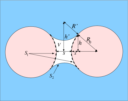
Figure 10: Sketch of two spherical solutes of radius $R_{0}$ at a surface-to-surface distance $s$. The white volume $V$ between the solutes approximates the region depleted of water. $S_{1}$ and $S_{2}$ are the surrounding solute-vapor and liquid-vapor surface areas, resp. $R^{\prime}$ is the radius of the curved surface $S_{2}$.

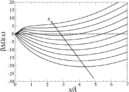
Figure 11: Free energy $\Delta\Omega$ of dried states between neutral spherical solutes with radius $R_{0}=10$ according to Eq. (11). The volume of the empty state is described by the parameter $x$ for a given geometry, see Fig. 10. The most bottom curve is for a surface-to-surface distance $s=0$, then $s$ is incremented by 0.5Å  steps.

The difference in grand potential between the “dry” and filled states is then given (in absence of the electric charges) by the following generalization of Eq. (8):

$$\Delta\Omega=\rho_{l}\delta\mu V(x)-\gamma_{\rm s}S_{1}(x)+\gamma S_{2}(x),$$ (11)

where $\gamma_{s}$ is the surface tension of the solute-liquid interface and $\gamma$ the liquid-vapor surface tension. The first term in Eq. (11) is the bulk free energy for creating a cavity of volume $V(x)$ in water, and favors the filled state. Again, near liquid-vapor equilibrium $\delta\mu\ll k_{B}T$, and the volume term may be safely neglected. The second and third terms in Eq. (11) are the surface free energies for decreasing the solute-liquid and increasing the liquid-vapor interface, respectively. For simplicity we first assume $\gamma=\gamma_{s}$Huang et al. (2001); effects arising from $\gamma\neq\gamma_{s}$ will be discussed later. In the following we use the liquid-vapor surface tension of water $\gamma=0.174k_{B}T{\rm\AA}^{-2}$. $\Delta\Omega(x)$ is plotted versus the geometric control parameter $x$ in Fig. 11 for a solute of radius $R_{0}=1$nm, and various surface-to-surface distances $s$. At contact ($s=0$), $\Delta\Omega(x)$ exhibits a single negative minimum at the non-zero value $x=x_{\rm min}(s=0)$ signaling that the “dry” state with volume $V(x_{\rm min})$ is stable. As $s$ increases, the global minimum is raised to less negative energy values and occurs at smaller values of $x$, while a second local minimum appears at $x=0$, corresponding to a metastable, filled state. At the critical value $s_{c}\simeq 3.2$Å, the global minimum jumps from the non zero value of $x$ to $x=x_{\rm min}(s_{c})=0$. For $s>s_{c}$, the filled state is favored. The effective interaction $w(s)$ between two solutes is equal to the free energy difference in bringing them from infinite separation to a surface-to-surface distance $s$, and is given by Eq. (11), i.e. $w(s)=\Delta\Omega(s;x_{\rm min}(s))$. The energy at the global minimum is negative for all $s<s_{c}$ ($x_{\rm min}>0$), so that the interaction is always attractive. $s_{c}$ is the range of the interaction; at $s=s_{c}$, $w(s)=\Delta\Omega=0$, and $\gamma_{\rm s}S_{1}=\gamma S_{2}$.

The effective potentials and forces between two solutes of different radii $R_{0}=5,8,10,12$Å  from Eq. (11) are plotted in Fig. 12. A detailed numerical investigation shows that, assuming $\gamma_{s}=\gamma$, the range of the potential (and of the resulting effective force) is $s_{c}\simeq 0.32R_{0}$, scaling linearly with solute radius, independently of $\gamma$. The contact value of the potential is $w(0)\simeq-1.19\gamma R_{0}^{2}$, scaling with the solute surface area. The contact value of the force is $F(0)\simeq-4.28\gamma R_{0}$. The force increases roughly linearly with a slope independent of $R_{0}$ (cf. Fig. 12). The results are accurately represented by

$$F(s)=\gamma\begin{cases}-a_{1}R_{0}+a_{2}s&{\text{for}}\,\,s\leq s_{c}=a_{3}R_{0};\cr 0&{\rm otherwise}.\cr\end{cases}$$ (12)

and

$$w(s)=\gamma\begin{cases}-a_{0}R_{0}^{2}+a_{1}R_{0}s-\frac{a_{2}}{2}s^{2}&{\text{for}}\,\,s\leq s_{c};\cr 0&{\rm otherwise}.\cr\end{cases}$$ (13)

with $a_{0}=1.19$, $a_{1}=4.28$, $a_{3}=0.32$, and $s_{c}=a_{3}R_{0}$. If the force is assumed to be linear in $s$, $a_{2}$ is fixed by the other constants according to $a_{2}=2(a_{1}a_{3}-a_{0})/a_{3}^{2}\simeq 3.51$. The linear scaling of the contact value of the force with solute radius $R$ may be rationalized by a simple consideration of the potential of mean force for plates ($R=\infty$) at contact, $w(0)=-2\gamma$ and an application of the Derjaguin approximation, valid for weakly curved substrates (i.e. large $R$); Louis et al. (2002) this leads to the estimate $F(s=0)=-2\pi R\gamma$, which indeed predicts linear scaling.

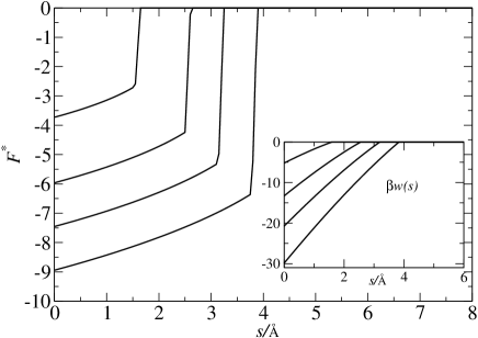
Figure 12: Results from the phenomenological theory in section IV.2 for the mean force, $F^{*}=\beta F$Å, between two neutral ($q=0$) spheres in SPC/E water. Results are plotted for solute radii $R_{0}=5$Å , $R_{0}=8$Å , $R_{0}=10$Å , and $R_{0}=12$Å . The inset shows the integrated force (potential of mean force). The depth and range of the force and potential increases with $R$.

Near a “realistic” solute, water will have a surface tension $\gamma_{s}\neq\gamma$, due to Van-der-Waals and electrostatic interactions, as well as the influence of curvature for small solutes. One may expect $\gamma_{s}<\gamma$, and lowering $\gamma_{s}$ will lead to less hydrophobic attraction. A possible approach to include the electrostatic field effects due to a net charge on the solutes is to absorb these effects into the solute-liquid surface tension. A naive procedure is to approximate $\gamma_{s}$ by the solvation free energy per unit area of a charged solute. In section III.2 it was shown that the Born expression (4) fits the MD data for uniformly charged solutes quite well, once the Born radius $R_{B}$ has been adjusted. Thus one may write for large solutes $R\gtrsim 1$nm (neglecting $1/\epsilon$ compared to 1):

$$\gamma_{s}=\gamma-\frac{q^{2}e^{2}}{32\pi^{2}\epsilon_{0}R_{B}^{3}},$$ (14)

which indeed lowers the hydrophobic attraction when charge is added to the solutes. No hydrophobic attraction occurs when $\gamma_{s}=0$, so that the corresponding critical charge $q_{c}$ satisfies:

$${q_{c}^{2}}={32\pi^{2}e^{2}\epsilon_{0}\gamma R_{B}^{3}}$$ (15)

For $R_{B}\approx 1$nm, one obtains $|q_{c}|\approx 3$, which in view of the sensitivity to $R_{B}$, yields at least the right order of magnitude, since the MD data discussed later suggest $|q_{c}|\approx 8$.

IV.3 Forces and potentials from simulation

In the MD simulations, the mean force between two solutes was calculated by placing them at fixed positions ${{\vec{R}}_{1}}$ and ${{\vec{R}}_{2}}$ along the body diagonal of the simulation cell, and averaging over water configurations generated during the runs which extended typically over 1-3 ns. The averaging was performed as long the statistical error was larger than $\Delta\beta F{\rm\AA}=0.5$, approximately twice the symbol size in the figures showing the forces. Separate MD simulations have to be carried out for each center-to-center distance ${{\vec{R}}_{12}}={{\vec{R}}_{1}}-{{\vec{R}}_{2}}$, i.e. for a series of surface-to-surface distances $s=R_{12}-2R_{0}$. The force acting on solute 1 is estimated from the statistical average of the gradient of the total interaction energy $V_{\rm sol}$ in Eq. (2):

$${\vec{F}}_{1}(R_{12})=\left\langle-\nabla V_{\rm sol}(R_{12})\right\rangle_{{\vec{R}}_{12}},$$ (16)

where the constrained statistical average is taken over solvent configurations, when the two solutes are held fixed at a separation $\vec{R}_{12}$. Note that while the solute translational degrees are frozen, they rotate freely under the action of the torques exerted by the solvent and the other solute. In other words, the calculated effective forces are orientationally averaged. By symmetry, $\vec{F}_{2}(\vec{R}_{12})=-\vec{F}_{1}(\vec{R}_{12})$. The magnitude of the effective force is obtained by projecting onto the vector $\vec{R}_{12}$:

$$F(R_{12})=\frac{{\vec{R}}_{1}-{\vec{R}}_{2}}{R_{12}}\cdot{\vec{F}}_{1}(R_{12}).$$ (17)

The resulting effective solute-solute potential follows from:

$$w(R_{12})=\int_{R_{12}}^{\infty}F(R)dR.$$ (18)

In simulations where counterions are present, the sum of all pair interactions between the latter and the solute must be added to $V_{\rm sol}$ in Eq. (16), i.e. the mean force acting on the solute is the statistical average of the sum of the instantaneous forces exerted by all water molecules and ions on the solute, in the presence of a fixed second solute.

V Molecular dynamics results for profiles and forces

V.1 Neutral solutes

We first consider the case of uncharged solutes. The water density profiles are illustrated in Figs. 13(a)-(e) for the case of solutes of radius $R=11$Å  and different surface-to-surface distances along the $z$-axis joining the centers. We plot density contours coded by variable shades of gray. The profiles are calculated using a cylindrical average around the symmetry axis (center-to-center line). The profiles show a considerable depletion (dark region) of the solvent between the spheres, reminiscent of the observations of Wallquist and Berne for flatter solutes. Wallquist and Berne (1995) As the surface-to-surface distance $s$ is increased for fixed radius $R$, the water molecules penetrate into the region between opposite solute surfaces, as signaled by a decreasing radius of the dark region between the spheres. Eventually at a distance between $s\approx 5$Å  and 6Å  (Figs. 13(c) and (d)) the region between the solutes fills with liquid. When $s\gtrsim 7$Å, the solvent layers around an isolated solute are hardly disturbed by the presence of the other solute.

Examples for the mean force for several radii 6Å $\leq R\leq 13$Å  are shown in Fig. 14. The largest radii are of the order of the size of small globular proteins or of oil-in-water micelles. The average force obviously goes to zero at large distances $s$ and for symmetry reasons, it is directed along the center-to-center axis. As expected from a depletion mechanism, the force is attractive and its contact values and range increase with $R$. We observe for all radii that the range of the force is similar to the distance at which the drying between the solutes vanishes. The potentials of mean force $w(s)$ may be calculated for each $R$ according to Eq. (18). The resulting potentials are shown in the inset to Fig. 14. They closely resemble results obtained for polymer-induced depletion potentials between spherical colloids, albeit on different length and energy scales.Louis et al. (2002) The force at contact, $F(s=0)$, and the range of the force $s_{c}$ scales roughly with $R$ in agreement with the macroscopic model prediction (14). From the MD data we extract a rough scaling $F(s=0)\approx 3.9\gamma R$ and range $s_{c}\approx 0.4R$, reasonably close to the theoretical estimates from Sec. IV.B. Overall there is a striking qualitative and even semi-quantitative agreement between the MD forces in Fig. 14 and the predictions of tbe macroscopic model in Fig. 12.

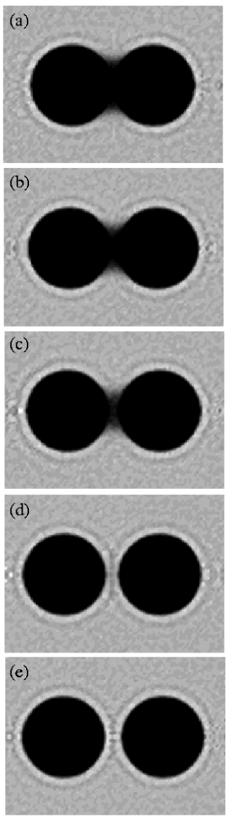
Figure 13: Contour density profiles of water around two neutral ${\rm S}_{0}$ solutes with radius $R=11$Å  for surface-to-surface distances (a) $s=2$Å, (b) $s=4$Å, (c) $s=5$Å, (d) $s=6$Å, and (e) $s=7$Å. The dark and light areas correspond to low and high densities of water molecules.

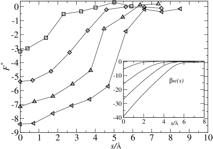
Figure 14: Simulation results (symbols) of the mean force, $F^{*}=\beta F$Å, between two neutral ${\rm S}_{0}$ solutes in SPC/E water. The lines are guides to the eye. Results are plotted for solute radii $R=6$Å  (squares), $R=9$Å  (diamonds), $R=11$Å  (triangles pointing up), and $R=13$Å  (triangles pointing left). The inset shows the integrated force (potential of mean force) in obvious order.

V.2 Uniformly charged solutes

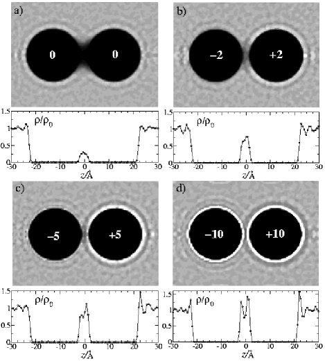
Figure 15: Density profiles of the water molecules around (a) two neutral ${\rm S}_{0}$ solutes of radius $R=11$Å  and two oppositely charged ${\rm S}_{\pm}$ solutes of radius $R=11$Å  carrying a charge $\pm qe$ with (b) $|q|=2$, (c) $|q|=5$, and (d) $|q|=10$. The surface-to-surface distance in all cases is $s=4$Å. In the contour plots dark regions indicate low density regions while high densities are plotted bright. The panels below the contour plots show the water density $\rho$ scaled with water bulk density $\rho_{0}$ in a cylinder of radius $5$Å, coaxial with the center-to-center line of the solutes.

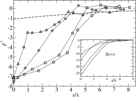
Figure 16: Mean force, $F^{*}=\beta F$Å, as a function of surface-to-surface distance $s$ for neutral ${\rm S}_{0}$ solutes (circles) and oppositely charged ${\rm S}_{\pm}$ solutes of $R=11$Å  with different central charges $\pm qe$: $q=2$ (squares), $q=5$ (diamonds), $q=10$ (triangles up). The dashed line represents the electrostatic force between 2 periodically repeated solutes with opposite charges $q=\pm$ 10 in a continuous solvent with permittivity $\epsilon=80$. The inset shows the resulting potentials of mean force; the contact values $w(s=0)$ increase with $q$.

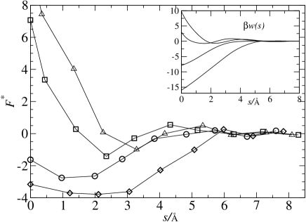
Figure 17: Mean force, $F^{*}=\beta F$Å, as a function of surface-to-surface distance $s$ for equally charged ${\rm S}_{\pm}$ solutes of radius $R=11$Å  and $q=-4$ (diamonds), $q=4$ (circles), $q=-8$ (squares), and $q=8$ (triangles). The inset shows the according potential of mean force.

We now turn to charged solutes. Consider first oppositely charged solutes. The water density profiles are illustrated in Figs. 15(a)-(d) for the case of solutes of radius $R=11$Å , a surface-to-surface distance $s=4$Å , and various charges $q$. The upper part of each frame shows a density contour plot coded by variable shades of gray. The lower part shows density profiles along the center-to-center axis $z$, averaged over a coaxial cylindrical volume of radius $5$Å. In Frame (a) we plot the density distribution for the neutral case $Q=0$ for comparison with the charged systems. Frames (b)-(d) in Fig. 15 show water density profiles in the vicinity of two spheres carrying opposite electric charges $\pm qe$ at their center (opposite charges ensure overall charge neutrality without any need for counterions). As $q$ increases from zero (frame (a)), water is seen to penetrate between the two solutes, the central peak around $z=0$ in the density profiles increases rapidly and its amplitude reaches roughly the bulk density of water when $q=10$. Note that this central peak is asymmetrically split, indicating the presence of two hydration layers which differ somewhat depending on their association with the anionic or cationic solute. This difference is also evident in the contact values of the outside surfaces of the solutes, and is a consequence of the different arrangements of the water dipoles around the solutes induced by the local electric fields. The asymmetry of the profiles can be rationalized by inspecting the water structure around isolated solutes, as shown in Fig. 5(a) and (b) and Fig. 4 in Sec. III.1. The hydration shell is more sharply defined around the cationic than around the anionic solute. The water dipoles tend to point radially away from the cation, while the opposite configuration is more favorable around anions.

The resulting mean forces between solutes are plotted for $q=0,2,5$ and 10, as functions of the surface-to-surface distance $s$ in Fig. 16 together with corresponding potentials of mean force. The mean force includes the direct Coulomb interaction between the two solutes (with proper account for the periodic images), which is in fact an order of magnitude larger than the total mean force. At large distances hydrophobic interactions become negligible and the force should tend to $-q^{2}e^{2}/(4\pi\epsilon_{0}\epsilon r^{2})$, where $r=2R+s$ and $\epsilon$ is the dielectric permittivity of bulk water; the corresponding curve for $q=\pm 10$ is also shown in Fig. 16.

The most striking result illustrated in Fig. 16 is the near independence of the force at contact, $s=0$, with respect to solute charge. From the density profiles in Fig. 15 the hydrophobic attraction is expected to be reduced but this reduction is almost exactly compensated by the Coulomb attraction between solutes in the presence of the solvent. As $q$ increases, the initial slope of the effective force increases. The potential of mean force (shown in the inset to Fig. 16) exhibits a contact value which increases with $q$, indicating that the reduction of hydrophobic attractive free energy clearly outweighs the increase in bare Coulomb attraction between the latter. Simulations calculating the forces at and near contact for $q=7$ and $q=15$, not shown in Fig. 16, confirm this trend. Note that the potential of mean force for $q=10$ shows more long range attraction compared to the smaller $q$ data due to the increased electrostatic attraction. The eye-catching kink in the force for $q=$10, at a distance $s\approx 1$Å  is reproducible, and is probably related to the pronounced shell structure of water molecules around highly charged solutes, discussed in sec III.1. While for neutral (and weakly charged) solutes, the O and H density profiles show little structure, they are sharply peaked at a distance $s\approx 1$Å  of the O atoms from the solute surface. This would lead to a complete shared hydration layer, and consequently to a kink in the force versus distance curve, between 2 flat solutes separated by $s=2$Å . This critical separation is shifted to shorter distances due to the curvature of spherical solutes.

In view of this delicate balance between various interactions, we have also examined the case of equally charged solutes. In this case monovalent counterions (Na⁺ or Cl^-) were included to ensure overall charge neutrality. The situation is summarized in Fig. 17 for solutes of radius $R=11$Å  and charge $q=\pm 4$ and $q=\pm 8$. Charges of 4 and 8 were chosen to allow a direct comparison with the results for the models ${\rm T}_{\pm}$ and ${\rm C}_{\pm}$ in the next section. The water density profiles are symmetric with respect to $z=0$ for equally charged solutes, but differ substantially when going from a pair of anions to a pair of cations, as discussed in Sec. III.1. This difference is reflected in the effective forces and potentials shown in Fig. 17. The interaction between the anionic solutes is always more attractive. For $q=\pm 4$ hydrophobic attraction overcomes the repulsion between like charges, while for $q\pm 8$ the electrostatic contribution dominates and the force is mainly repulsive, apart from a small attractive kink at $s=2-3$Å. The contact value of the repulsive forces is an order of magnitude higher than in a continuous solvent, originating obviously from the lack of water between the solutes and, hence a reduced dielectric screening.

The reduction of the hydrophobic attraction between initially uncharged solutes, upon increasing the solute charge, may be qualitatively understood by the orienting action of the strong electric field between charged solutes on the water molecules, which disrupts the local hydrogen-bond structure and moves water locally away from conditions of liquid-vapor coexistence, so that “drying” no longer occurs.

V.3 Discrete charge patterns

The water density distribution around two tetrahedral solutes ${\rm T}_{0}$ (i.e carrying no net charge) is plotted in Fig. 18(a)-(e) for increasing values of the surface-to-surface distance $s$. As in the case of neutral solutes ${\rm S}_{0}$, water depletion between the solutes is observable up to a solute distance of $s\simeq 5$Å. The bright regions near the surfaces indicate high density water and stem from the solvation shells in the immediate vicinity of the surface charges. We note again that the density profiles were calculated by averaging the water density cylindrically around the symmetry axis and the solutes were free to rotate in the simulations. The difference in brightness at the solute surfaces shows that certain orientational configurations are favored over others. If the tetrahedra were rotating freely (without any mutual interactions), the brightness would be the same everywhere on the solute contour, as in the case of homogeneously charged solutes. It seems that the systems chooses those configurations where the hydrophobic parts of the solutes (i.e. areas between the hydrophilic surface charges) face each other. We have also performed simulations of the overall neutral tetrahedral solute replacing the SPC/E water by a continuous solvent with permittivity $\epsilon=80$. In the latter case and for short distances, $s\lesssim 5$Å, configurations are favored in which opposite surface charges associated with the two solutes face each other, thus strongly lowering the electrostatic energy of the system. With explicit water this is apparently no longer the case, despite the expected reduction in dielectric screening close to the surfaces; the system tries to deplete water from the solute surfaces between the solutes. For distances larger than $s\simeq 5$Å , where no visible drying occurs, the positions of the bright regions are more smeared out on average, indicating a higher rotational freedom of the solutes. A simple configurational order parameter will be defined and discussed later. The water profiles for the tetrahedral solutes ${\rm T}_{+}$ show the same behavior, in particular a visible drying for $s\lesssim 5$Å. We have not performed simulations of a pair of the negative ${\rm T}_{-}$ tetrahedra but expect similar behavior.

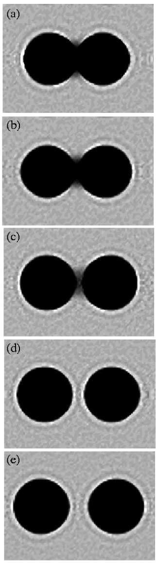
Figure 18: Contour density profiles of water around two ${\rm T}_{0}$ solutes for surface-to-surface distances (a) $s=0$Å, (b) $s=2$Å, (c) $s=4$Å, (d) $s=6$Å, and (e) $s=9$Å.

The water density profiles around a solute ${\rm C}_{0}$ carrying an overall neutral cubic charge distribution are plotted in Fig. 19(a)-(c). No water depletion is visible at any distance. In (a) the black region between the solutes comes from the fact that the solute surfaces touch. The positions of the high density regions of water corresponding to the first solvation shells of the surface charges are on average distributed homogeneously over the sphere surface, pointing to a high orientational freedom of the solutes. The density of water close to the solute surface (bright ring in Figs. 19(a)-(c)) is on average higher compared to the tetrahedra due to the larger surface charged density. The water density profiles for the positive cubic solute ${\rm C}_{+}$ show a different behavior, resembling the results for the tetrahedral solute, as shown in Fig. 20. For distances $s\lesssim 4$Å  no bright region is found between the solutes, and hence water depletion is observed. Similar to the tetrahedral case the solutes stay mainly in orientational configurations in which the hydrophobic patches face each other.

Figure 19: Contour density profiles of water around two ${\rm C}_{0}$ solutes with cubic charge distribution for surface-to-surface distances (a) $s=0$Å , (b) $s=2$Å , and (c) $s=4$Å .

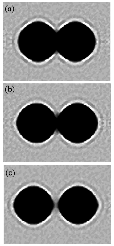
Figure 20: Contour density profiles of water around two ${\rm C}_{+}$ solutes for surface-to-surface distances (a) $s=0$Å , (b) $s=2$Å , and (c) $s=4$Å .

The effective force between the model solutes is plotted in Fig. 21. We show the force between pairs of neutral and overall positive tetrahedra, ${\rm T}_{0}$ and ${\rm T}_{+}$ as well as between pairs of neutral and overall positive cubes, ${\rm C}_{0}$ and ${\rm C}_{+}$. Simulations with overall charged solutes were carried out with explicit counterions. We have not performed simulations of a pair of overall negative tetrahedra and cubes. The force between pairs of overall neutral and charged tetrahedra is only slightly less attractive than between pairs of spherically symmetric neutral solutes (compare to Fig. 14). This is surprising as one expects a stronger influence of the high electric fields generated by the surface charges. We learned from the investigation of homogeneously charged solutes that an electric field can considerably lower the hydrophobic attraction. Apparently, a more anisotropic electric field distribution again favors hydrophobic attraction. Compare the force between pairs of positively charged tetrahedra and pairs of homogeneously charged solutes with the same overall charge $q=+4$ (Fig. 17): the attraction between the homogeneously charged solutes is less than half that between ${\rm T}_{+}$ solutes. As already discussed above, the strong attraction between two tetrahedra is accompanied by water depletion between them, as in the case of homogeneous neutral solutes. The water density profile around an isolated tetrahedral solute ${\rm T}_{\pm}$, shown in Sec. III.1, already illustrated strong depletion of water from the regions between the first solvation shells of the discrete surface charges. A possible explanation of the strong attraction between two tetrahedra is that this depletion is amplified when two hydrophobic patches of the solutes come close and face each other, and thus lowering the free energy.

The effective force between two solutes with overall neutral cubic charge distribution shows qualitative differences compared to the tetrahedra. Cubes with zero overall charge still attract each other, but the interaction range is decreased. Analysis of the configurations shows that for close cubic solutes ($s\approx 1-3$Å) one positive and one negative charge belonging to different solutes are on average very close, interacting with reduced dielectric screening than in bulk water due to their mutual proximity. The attraction observed is therefore mainly due to the electrostatic contribution and not hydrophobic attraction as in the case of neutral tetrahedra. For the ${\rm C}_{+}$ solute the situation is again different. All charges repel, allowing the hydrophobic patches to face each other and water depletion is induced, as seen in the water profiles of Fig. 20. Although equally charged, the cubic solutes still attract each other in striking contrast to the homogeneously charged solutes with $Q=8$ in explicit water (Fig. 17) and different to the case where water is replaced by a continuous solvent with $\epsilon=80$, also plotted in Fig. 21.

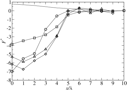
Figure 21: Mean force between ${\rm T}_{+}$ (diamonds), ${\rm T}_{0}$ (triangles), ${\rm C}_{+}$ (squares), and ${\rm C}_{0}$ (circles) solutes. Also plotted is the force between two periodically repeated ${\rm C}_{+}$ solutes in a continuous solvent with $\epsilon=80$ (solid line without symbols).

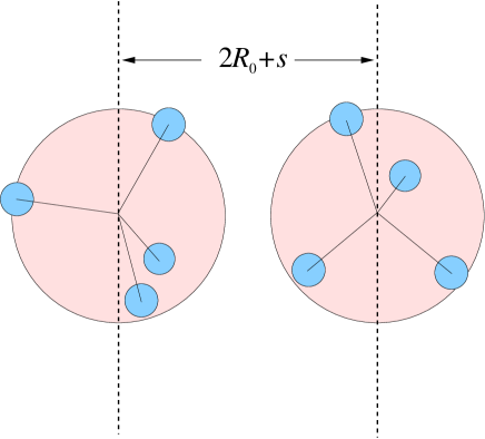
Figure 22: Sketch of two T solutes with radius $R_{0}$ and a surface-to-surface distance $s$. The dashed lines through the solute centers delimit a slab of width $2R_{0}+s$. The numbers of solute charges (small spheres) of each solute $N_{1}$ and $N_{2}$ inside the slab define the order parameter $N=N_{1}\cdot N_{2}$, described in section V.3. $N=6=3\cdot 2$ in the configuration shown.

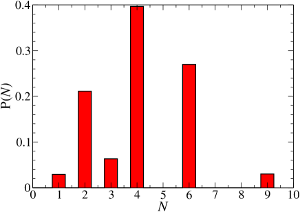
Figure 23: Configurational probabilities $P(N)$ as defined in Sec. V.3 for two non-interacting tetrahedral solutes.

In the following we investigate how the explicitly resolved water affects the average orientational configurations of two close tetrahedral solutes, when their centers are held at fixed positions. In a continuous solvent the probability of observing a certain configuration is purely determined by the electrostatic interactions between the surface charges. Obviously, for close distances of the solutes, structural effects of explicit water are expected to be very significant. A simple orientational order parameter, which coarsely probes different orientational configurations of a pair of tetrahedral solutes can be defined as follows: we count the number of surface charges in the slab delimited in width by the centers of the two solutes, as sketched in Fig. 22. Let $N_{1}$ and $N_{2}$ be the numbers of charges in the slab belonging to the first and second solutes. The values $N_{i}$, $i$=1,2 for a tetrahedron with four charged vertices are obviously $N_{i}=1,2$ or 3 (it is not possible to have four charges on one half sphere of the tetrahedral solute). The order parameter is now defined as the product $N=N_{1}N_{2}$ and can take values 1,2,3,4,6,9, which characterizes 6 different mutual orientational configurations. For $N=1$, for instance, one charge of each solute is located in the slab, and the charges are both necessarily close to the symmetry axis; on the other hand, when $N=9$, 3 charges of each solute are within the slab and the bare triangular surfaces between the three charges are mainly facing each other. In Fig. 22 we sketch two tetrahedra in a configuration $N=3\cdot 2=6$. The probability distribution $P(N)$ for two freely (without any interactions) rotating tetrahedra is plotted in Fig. 23. $N=2=2\cdot 1=1\cdot 2$, $N=4=2\cdot 2$, and $N=6=2\cdot 3=3\cdot 2$ are the most likely configurations, with probabilities $P(2)\simeq 0.21$, $P(4)=\simeq 0.4$, and $P(6)=0.28$.

In Fig. 24(a)-(d) we plot the probability distribution $P(N)$ for interacting tetrahedra in a continuous solvent with permittivity $\epsilon=80$. In Fig. 24(a) and (b) we show the result for a pair of overall neutral ${\rm T}_{0}$ solutes at distances $s=3$Å  and $s=9$Å . For the close distance the free rotator distribution is dramatically changed and the $N=1$ and $N=2$ configurations are strongly favored. This is due to negative and positive charges from different solutes attracting each other at close distance. For the larger distance the electrostatic interactions are weaker and $P(N)$ strongly resembles the free rotator distribution again. In Fig. 24(c) and (d) we show the same distribution function, now for a pair of overall positive solutes at distances $s=3$Å  and $s=9$Å , resp. Here, at close distance the $N=1$ and $N=2$ configurations are suppressed due to the proximity of like charges, and the $N>3$ configurations are enhanced, since they allow the charges of one solute to be at larger mean distance from the like charges of the second solute. For large distances, (d), we again recover the free rotator distribution.

In Fig. 25(a)-(d) the continuous solvent is now replaced by explicit water molecules. For close solutes ($s=3$Å) the difference with the continuous solvent is large: the probabilities of the $N=1$ and $N=2$ configurations are reduced both for the neutral (a) and overall charged tetrahedra (c). The $N=6$ and $N=9$ configurations are greatly enhanced, indicating that on average the are hydrophobic surfaces face each other, as expected from the water profiles in Fig. 18(b),(c). Remarkably, even for case (a) the explicit solvent system strongly favors water depletion rather than the proximity of two unlike charges, which would lower the electrostatic energy significantly. Increasing the distance to $s=9$Å, the probabilities of the $N=6$ and $N=9$ configurations are lowered and the overall distributions, both for neutral and positive tetrahedra are more similar to the free rotator distribution.

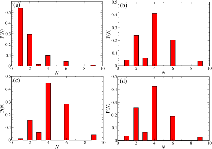
Figure 24: Configurational probabilities $P(N)$ as defined in Sec. V.3 for two tetrahedral solutes in a continuous solvent with $\epsilon=80$. (a) and (b) are for ${\rm T}_{0}$ solutes at a surface-to-surface distance $s=3$Å  and $s=9$Å. (c) and (d) are for ${\rm T}_{+}$ solutes at a distance $s=3$Å  and $s=9$Å, resp.

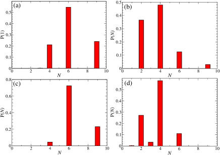
Figure 25: Same as in Fig. 24, but now with explicit SPC/E water instead of a continuous solvent.

VI Conclusion

We have used a simple model of neutral and charged, nanometer-sized spherical solutes, embedded in explicit aqueous solvent, to investigate the influence of charge patterns on the solvation of a single solute, and on the effective, solvent-induced interaction between two solutes. The charge patterns considered in this paper include uniform charge distributions (equivalent to a single charge at the center of the spherical solute), as well as tetrahedral or cubic charge distributions, involving 4 or 8 discrete positive or negative charges situated at the solute surface, adding up to an overall positive, zero or negative charge $Q$ (the ${\rm T}_{+},{\rm T}_{-},{\rm T}_{0}$ and ${\rm C}_{+},{\rm C}_{-},{\rm C}_{0}$ models).

Extensive constant pressure and constant temperature ($NPT$) Molecular Dynamics simulations were carried out under “normal” solvent conditions, i.e. close to liquid-vapor coexistence of water at room temperature. These simulations provide water density profiles around a single solute or a pair of solutes, which can be resolved into solute-oxygen and solute-hydrogen pair distribution functions, the distance resolved orientational order parameter $P(r)$, the solvation free energy as a function of solute radius and charge, as well as the effective force and pair potential between two solutes, averaged over solvent configurations. The main results of this investigation may be summarized as follows:

1. The density profiles of water around a single, neutral solute (${\rm S}_{0}$ model), and their variation with solute radius $R$ (cf. Fig. 3) exhibit the characteristic “destructuring” for radii $R\gtrsim 5$Å  already reported by earlier studies. Stilinger (1973); Huang et al. (2001); Lum et al. (1999) The water molecules exhibit no significant orientational ordering around neutral nano-sized solutes.

2. The hydrogen and oxygen density profiles change dramatically when the solute is uniformly charged (${\rm S}_{\pm}$ models). These profiles are sensitive to the anionic or cationic nature of the solute (for a given absolute charge $|Q|$), in addition the hydrogen profiles exhibit a splitting of the main peak in the case of anionic (${\rm S}_{-}$) solutes (cf. Fig. 5). The orientational order parameter $P(r)$ exhibits a significant structure, and a relatively slow decay with $r$, indicative of strong orientational ordering around the solutes ${\rm S}_{+}$ or ${\rm S}_{-}$, which is somewhat more pronounced around an anionic solute. The hydration asymmetry results in preferential solvation of anionic solutes for a given radius and absolute charge $|Q|$, in agreement with earlier findings. Hummer et al. (1996); Lynden-Bell and Rasaiah (1997); Rajamani et al. (2004)

3. Moving from uniformly charged solutes to discrete (tetrahedral or cubic) charge patterns, the hydration of nano-sized solutes is found to exhibit a strong angular modulation associated with the hydrophilic “patches” around the discrete surface charges, and hydrophobic “patches” in between (cf. Fig. 6). The conflicting hydration patterns lead to a surprising depletion of water around ${\rm T}_{+}$ or ${\rm T}_{-}$ solutes, compared to a neutral solute ${\rm S}_{0}$. The solvation free energy is found to be about 20 $\%$ lower for solutes with discrete charge patterns compared to that of uniformly charged solutes with the same overall charge (cf. Fig. 9).

4. The present simulations confirm the strong hydrophobic attraction between two neutral spherical nano-sized solutes linked to solvent “drying”, which was already reported earlier for similar models. The MD results for solute radii $R\gtrsim 5$Å  are nearly quantitatively reproduced by a simple calculation based on purely macroscopic considerations, and the force at solute-solute contact is found to scale roughly linearly with $R$.

5. The effective attraction between neutral solutes is strongly reduced, or turns into a repulsion, when the nano-sized solutes carry equal, uniform charge distributions. The total force has a repulsive electrostatic component, while examination of the water density profiles shows that the “drying” is mostly suppressed. The effective force is systematically less attractive (or more repulsive) between pairs of cationic solutes compared to anionic pairs (cf. Fig. 17). Turning to a pair of oppositely (but uniformly) charged solutes, the MD simulations show that the range of the effective attraction decreases when the absolute charge $|Q|$ increases, again in agreement with simple macroscopic considerations, but that the effective force at contact seems to be independent of $Q$, and equal to the hydrophobic force between neutral solutes; we have no explanation for this surprising observation.

6. The situation for discrete solute charge patterns is, not surprisingly, more complex, due to the competition between the resulting hydrophilic and hydrophobic “patches” on the solute surface. On average, some “drying” of water is observed, and the resulting mean force between solutes carrying tetrahedral or cubic patterns is once more attractive, despite the electrostatic repulsion (“like-charge attraction”). This effect is obviously incompatible with crude “implicit solvent” models.

7. The complete break-down of “implicit solvent” models, whereby the latter is replaced by a dielectric continuum, is further illustrated by the highly coarse-grained representation of the configurational probability density of two solutes carrying discrete charge distributions, introduced in Sec. V. The relative orientations of the surface charge patterns on the two solutes are completely different for explicit and implicit solvent models, particularly at short surface-to-surface distances $s$ (cf. Figs. 24 and 25).

The key message of the present work is that explicit solvent models are unavoidable for a proper description of the effective interactions between nano-sized solutes like proteins, and that the latter are extremely sensitive to the precise location of any electric charges carried by the solutes. Contrarily to effective interactions on larger colloidal scales, a generic coarse-graining strategy appears to be useless when solutes in the nanometer range are considered, and fully molecular models are required for realistic simulations.

VII Acknowledgments

JD acknowledges the financial support of EPSRC within the Portfolio Grant RG37352. We thank A. Archer and V. Ballenegger for useful discussions, and A.A. Louis for using the computer cluster Ice.

VIII Appendix A: Simulation details

The simulations were performed with the DLPOLY2 Smith and Forester (1999) package. The Berendsen barostat and thermostat Berendsen et al. (1984) were used to maintain the SPC/E water at a pressure of 1 bar and a temperature $T=300$K. For the simulations of the solutes with inhomogeneous charge distributions (T and C models) we used the rigid body algorithm with quaternions to properly account for the rotation of the anisotropic solutes. To this end we switched to an integration routine using the Nosé-Hoover barostat and thermostat, which turned out to be more stable in conjunction with quaternions. We carefully checked that both barostats give the same results by performing tests with bulk water, treated both with bond contraints and with the rigid body algorithm. Test runs using the Nosé-Hoover barostat and thermostat for the S models also showed no difference.

The simulation cell is a periodically repeated cube with a maximum boxlength of about $L=48$Å, containing up to $N_{\rm w}$=3000 water molecules, depending on the solute size. For simulations of one isolated solute we required that the surface-to-surface distance to the nearest image solute was 20Å, yielding a box size of $L=2R+20$Å. For the calculation of the interaction force between two solutes, the latter are placed at fixed positions ${{\vec{R}}_{1}}$ and ${{\vec{R}}_{2}}$ on the body diagonal of the simulation cell. The center to center distance is then ${R_{12}}={|{\vec{R}}_{1}}-{{\vec{R}}_{2}}|$. The corresponding box dimensions are chosen such that the surface-to-surface distance $s={R_{12}}-2R_{0}$ to the nearest image solute is 20Å. The box length can be calculated as $L=(4R+s+20{\rm\AA})/\sqrt{3}$. Due to the constant pressure constraint the box length fluctuates slightly in the simulations. The long range electrostatic interactions were evaluated with smooth particle-mesh Ewald (SPME) summations Essmann et al. (1995) using 16 $\vec{k}$ vectors in each direction and a convergence parameter of 3.2$/r_{\rm cut}$. A cutoff distance $r_{\rm cut}=9$Å  was used for LJ-interactions and the real space SPME contributions. For the nanosized solutes a larger cut-off radius is obviously required. We optimize the computational speed by introducing a second cutoff for the solute-water and solute-ion interactions, chosen to be $R_{0}+4$Å, sufficient large for the shifted, short ranged repulsive interaction (1).

IX Appendix B: Finite corrections for solvation free energies from simulation

Accurate solavtion free energies for charged solutes can be obtained by Ewald summations in periodic cellsHansen (1986) when the self-interacion energy of the solute charges with its periodic images and the background charge is properly included.Hummer et al. (1996) This correction is slightly modified when the solute size $R$ is comparable to the box size $L$.Hummer et al. (1997) The final expression for the electrostatic contribution to the solvation free energy for our solute models, including the finite size corrections, is:

$$\Delta\mu_{\pm} = \Delta\mu_{\pm}^{\rm sim}$$ (19)

$$+ \frac{e^{2}}{8\pi\epsilon_{0}}\frac{\epsilon-1}{\epsilon}\left(\frac{\xi_{\rm EW}}{L}\sum_{\alpha=1}^{N_{\rm c}}q_{\alpha}^{2}+\frac{2\pi R^{2}}{3L^{3}}\sum_{\alpha=1}^{N_{\rm c}}q_{\alpha}^{2}\right)$$

$$+ \frac{e^{2}}{8\pi\epsilon_{0}}\frac{\epsilon-1}{\epsilon}\sum_{\alpha=1}^{N_{\rm c}}\sum_{\beta\neq\alpha,1}^{N_{\rm c}}q_{\alpha}q_{\beta}\left(\phi_{\rm EW}(\vec{r}_{\alpha\beta})-\frac{1}{|\vec{r}_{\alpha\beta}|}\right),$$

where $\epsilon$ is the macroscopic permittivity of water, and for a periodic array of cubic simulation cells, $\xi_{EW}\approx-2.837297$. In the case of a uniformly charged solute corresponding to a single charged site $qe$ at the center, the result (LABEL:eq:correct) reduces toHummer et al. (1997)

$$\Delta\mu_{\pm}=\Delta\mu_{\pm}^{\rm sim}+\frac{q^{2}e^{2}}{8\pi\epsilon_{0}}\frac{\epsilon-1}{\epsilon}\left(\frac{\xi_{\rm EW}}{L}+\frac{2\pi R^{2}}{3L^{3}}\right).$$ (22)

With the system sizes used in the present simulation the finite size corrections are very large and represent typically twice the value of $\Delta\mu_{\rm sim}$ and stem mainly from the $\xi_{\rm EW}$-term in Eqs. (19) and (20).

References

- Rubinstein and Colby (2003) M. Rubinstein and R. H. Colby, Polymer Physics (Oxford University Press, 2003).
- Chandler (2004) D. Chandler (2004), to appear in Nature.
- Likos (2001) C. N. Likos, Phys. Rep. 348, 267 (2001).
- Stilinger (1973) F. H. Stilinger, J. Solution Chem. 2, 141 (1973).
- Hummer and Garde (1998) G. Hummer and S. Garde, Phys. Rev. Lett. 80, 4193 (1998).
- Lum et al. (1999) K. Lum, D. Chandler, and J. D. Weeks, J. Phys. Chem. B 103, 4570 (1999).
- Huang et al. (2001) D. M. Huang, P. L. Geissler, and D. Chandler, J. Phys. Chem. B 105, 6704 (2001).
- Wallquist and Berne (1995) A. Wallquist and B. J. Berne, J. Phys. Chem. 99, 2893 (1995).
- Shinto et al. (1999) H. Shinto, M. Miyahara, and K. Higashitani, J. Coll. Interface Sci. 209, 79 (1999).
- Kinoshita et al. (1996) M. Kinoshita, S. Iba, K. Kuwamoto, and M. Harada, J. Chem. Phys. 105, 7177 (1996).
- Qin and Fichthorn (2003) Y. Qin and K. A. Fichthorn, J. Chem. Phys. 119, 9745 (2003).
- Allahyarov et al. (2002) E. Allahyarov, H. Löwen, A. Louis, and J. Hansen, Europhys. Lett. 57, 731 (2002).
- Berendsen et al. (1987) H. J. C. Berendsen, J. R. Grigera, and T. P. Straatsma, J. Phys. Chem. 91, 6269 (1987).
- Dzubiella and Hansen (2003) J. Dzubiella and J.-P. Hansen, J. Chem. Phys. 119, 12049 (2003).
- Spohr (1999) E. Spohr, Electrochim. Acta 44, 1697 (1999).
- Essmann et al. (1995) U. Essmann, L. Perera, M. L. Berkowitz, T. Darden, H. Lee, and L. G. Pedersen, J. Chem. Phys. 103, 8577 (1995).
- Smith and Forester (1999) W. Smith and T. R. Forester (1999), the DLPOLY_2 User Manual.
- Frenkel and Smit (1996) D. Frenkel and B. Smit, Understanding Molecular Simulation: From Algorithms to Applications (Academic Press, 1996).
- Born (1920) M. Born, Z. Phys. 1, 45 (1920).
- Reiss et al. (1959) H. Reiss, H. L. Frisch, and J. L. Lebowitz, J. Chem. Phys. 31, 369 (1959).
- Latimer et al. (1939) W. M. Latimer, K. S. Pitzer, and C. M. Slansky, J. Chem. Phys. 7, 108 (1939).
- Hummer et al. (1996) G. Hummer, L. Pratt, and A. E. Garcia, J. Phys. Chem. 100, 1206 (1996).
- Hummer et al. (1997) G. Hummer, L. Pratt, and A. E. Garcia, J. Chem. Phys. 107, 9275 (1997).
- Lynden-Bell and Rasaiah (1997) R. M. Lynden-Bell and J. C. Rasaiah, J. Chem. Phys. 107, 1981 (1997).
- Rajamani et al. (2004) S. Rajamani, T. Ghosh, and S. Garde, J. Chem. Phys. 120, 4457 (2004).
- Bolhuis and Chandler (2000) P. G. Bolhuis and D. Chandler, J. Chem. Phys. 113, 8154 (2000).
- Louis et al. (2002) A. A. Louis, P. G. Bolhuis, and J. P. Hansen, J. Chem. Phys. 117, 1893 (2002).
- Berendsen et al. (1984) H. J. C. Berendsen, J. P. M. Postma, W. F. van Gunsteren, A. DiNola, and J. R. Haak, J. Chem. Phys. 81, 3684 (1984).
- Hansen (1986) J.-P. Hansen, Molecular Dynamics Simulation of Statistical Mechanical Systems (North Holland, Amsterdam, 1986), edited by G. Ciccotti and W.G. Hoover.