Power Law Distribution of Wealth in a Money-Based Model

Abstract

A money-based model for the power law distribution (PLD) of wealth in an economically interacting population is introduced. The basic feature of our model is concentrating on the capital movements and avoiding the complexity of micro behaviors of individuals. It is proposed as an extension of the Equíluz and Zimmermann’s (EZ) model for crowding and information transmission in financial markets. Still, we must emphasize that in EZ model the PLD without exponential correction is obtained only for a particular parameter, while our pattern will give it within a wide range. The Zipf exponent depends on the parameters in a nontrivial way and is exactly calculated in this paper.

I Introduction

Many real life distributions, including wealth allocation in individuals, sizes of human settlements, website popularity, words ranked by frequency in a random corpus of text, observe the Zipf law. Empirical evidence of the Zipf distribution of wealth [1-9] has recently attracted a lot of interest of economists and physicists. To understand the micro mechanism of this challenging problem, various models have been proposed. One type of them is based on the so-called multiplicative random process[10-21]. In this approach, individual wealth is multiplicatively updated by a random and independent factor. A very nice power law is given, however, this approach essentially does not contain interactions among individuals, which are responsible for the economic structure and aggregate behavior. Another pattern takes into account the interaction between two individuals that results in a redistribution of their assets[22-25]. Unfortunately, some attempts only give Boltzmann-Gibbs distribution of assets[24,25], while some others[23], though exhibiting Zipf distributions, fail to provide a stationary state.

In this paper, we shall introduce a new perspective to understand this problem. Our model is based on the following observations: (i) In order to minimize costs and maximize profits, two corporations/economic entities may combine into one. This phenomenon occurs frequently in real economic world. Simply fixing attention on capital movements, we can equally say that two capitals combine into one.(ii) The disassociation of an economic entity into many small sections or individuals is also commonplace. The bankruptcy of a corporation, for instance, can be effectively classified into this category. Allocating a fraction of assets for the employee’s salary, a company also serves as a good example for the fragmentation of capitals. Under some appropriate assumptions, we shall establish a money-based model which is essentially an extension of the Eguíluz and Zimmermann’s (EZ) model for crowding and information transmission in financial marketsez1 ; ez2 . The size of a cluster there is now identified as the wealth of an agent here. However, analytical results will show that our model is quite different from EZ’s ez2 , which gives PLD with an exponential cut-off that vanishes only for a particular parameter. Here, a Zipf distribution of wealth is obtained within a wide range of parameters, and surprisingly, without exponential correction. The Zipf exponent can be analytically calculated and is found to have a nontrivial dependence on our model parameters.

This paper is organized as follows: In section 2, the model is described and the corresponding master equation is provided directly. In section 3, we shall present our analytical calculation of the Zipf exponent. Next, we give numerical studies for the master equation, which are in excellent agreement with analytic results. In section 5, the relevance of our model to the real world are discussed.

II the model

The money-based model contains $N$ units of money, where $N$ is fixed. Though in real economic environment the total wealth is quite possible to fluctuate, our assumption is not oversimplified but reasonable, given that the production and consumption processes are simultaneous and the resource is finite. The $N$ units of money are then allocated to $M$ agents (or say, economic entities), where $M$ is changeable with the passage of time. For simplicity, we may choose the initial state containing just $N$ agents, each with one unit of capital. The state of system is mainly described by $n_{s}$, which denotes the number of agents with $s$ units of money. The evolution of the system is under following rules: At each time step, a unit of money, instead of an agent, is selected at random. Notice that our model is much more concentrating on the capital movement among agents rather than the agents themselves. With probability $a\gamma/s$, the agent who owns this unit of money is disassociated, here $s$ is the amount of capitals owned by this agent and $\gamma$ is a constant which implies the relative magnitude of dissociative possibility at a macro level. After disassociation, this $s$ units of money are redistributed to $s$ new agents, each with just one unit. It must be illuminated that an real economic entity in most cases does not separate in such an equally minimal way. However, with a point of statistical view and considering analytical facility, this simplified hypothesis is acceptable for original study. Now, continue with our evolution rules. With probability $a(1-\gamma/s)$, nothing is done. And with probability $1-a$, another unit of money is selected randomly from the wealth pool. If these two units are occupied by different agents, then the two agents with all their money combine into one; otherwise, nothing occurs. Thus, $1-a$ in our model is a factor reflecting the possibility for incorporation at a macro level.

One may find that as $a$ is close to 1 and $\gamma$ is not too small, a financial oligarch is almost forbidden to emerge in the evolution of the system; but, if the initial state contains any figure such as Henry Ford or Bill Gates, he is preferentially protected. Note that the bankruptcy probability of moneybags is inverse proportional to their wealth ranks, and the possibility of being chosen is proportional to $sn_{s}/N$; thus, the Doomsday of a tycoon comes with possibility $an_{s}\gamma/N$, which is extremely small for large $s$. Meanwhile, the vast majority, if initially poor, is perpetually in poverty, with no chance to raise the economic status any way. In addition, if middle class exists at first, it will not disappear or expand in the foreseeable future. Again, it may be interesting to argue that when $a$ is slightly above zero, the merger process is prevailing and overwhelming, and all the capitals are inclined to converge. In this case, though the rich are preferentially protected, the trend in the long run is to annihilate them until the last. Of course, one-agent game is trivial. Likewise, it is not appealing to observe the system when $\gamma$ goes to 0 and $a$ to 1, since both merger and disintegration are nearly impossible–in other words, all the capitals are locked, thus the wealth pool is dead at any time.

Following Refs.ez2 ; x1 ; x2 in the case of $N\gg 1$, we give the master equation for $n_{s}$

$${\partial n_{s}\over\partial t}={1-a\over N}\sum_{r=1}^{s-1}rn_{r}(s-r)n_{s-r}-2(1-a)sn_{s}-asn_{s}{\gamma\over s}$$ (1)

for $s>1$ and

$${\partial n_{1}\over\partial t} =-2(1-a)n_{1}+a\sum_{s=2}^{\infty}s^{2}n_{s}{\gamma\over s}$$ (2)

$$=-2(1-a)n_{1}+a\gamma(N-n_{1})$$

where the identity

$$\sum_{s=1}^{\infty}sn_{s}=N$$ (3)

has been used. We must point out that Eq.(1) is almost the same as the master equation derived in Ref.ez2 for the EZ model except for an additional factor $\gamma/s$ in the third term on the right hand side of Eq.(1). Notice that this term is significant because otherwise the frequency of the disintegration for large $s$ agents would be too high.

Now we introduce $h_{s}=sn_{s}/N$, which indicates the ratio of wealth occupied by agents in rank $s$ to the total wealth, and $\alpha=a\gamma/2(1-a)$, that represents the maximum ratio of the disintegration possibility to the merger probability in the whole economic environment. Then, one can give the equations for the stationary state in a terse form:

$$h_{s}={s\over 2(s+\alpha)}\sum_{r=1}^{s-1}h_{r}h_{s-r}$$ (4)

and

$$h_{1}={\alpha\over 1+\alpha}$$ (5)

According to the definition of $h_{s}$, it should satisfy the normalization condition Eq.(3)

$$\sum_{s=1}^{\infty}h_{s}=1$$ (6)

When $\alpha$ is less than a critical value $\alpha_{c}=4$ which will be determined numerically in section 4, one can show that Eqs.(4-5) does not satisfy the normalization condition Eq.(3). This inconsistency implies that when $\alpha<\alpha_{c}$ the state with one agent who has all the $N$ units of money becomes importantx1 ; x2 . In this case, the finite-size effect and the fluctuation effect become nontrivial and the master equations (1-3) is no longer applicable to describe the systemx1 ; x2 . In this paper, we shall restrict our discussion to the case $\alpha>\alpha_{c}$.

III Analytic results

When $\alpha>\alpha_{c}$, one can show that $h_{s}\to A/s^{\eta}$ for sufficiently large $s$ with

$$\eta={\alpha\over\sum_{r=1}^{\infty}rh_{r}}$$ (7)

Notice that this equation is only consistent when $\eta>2$ because otherwise the sum $\sum_{r=1}^{\infty}rh_{r}$ would be divergent, and thus $h_{s}\to A/s^{\eta}$ becomes an inconsistent formula.

The derivation of Eq.(7) is described as follows: When $s$ is sufficiently large

$$h_{s} ={s\over 2(s+\alpha)}\sum_{r=1}^{s-1}h_{r}h_{s-r}$$ (8)

$$\approx{s\over s+\alpha}(\sum_{r=1}^{s^{\delta}}h_{s-r}h_{r}+h_{s}O({1\over s^{2\delta\eta-1-\eta}}))$$

$$\approx{s\over s+\alpha}\sum_{r=1}^{s^{\delta}}(h_{s}-{dh_{s}\over ds}r)h_{r}$$

$$\approx(1-{\alpha\over s})[h_{s}\sum_{r=1}^{\infty}h_{r}-{dh_{s}\over ds}\sum_{r=1}^{\infty}rh_{r}]+h_{s}O({1\over s^{\delta(\eta-1)}})$$

$$\approx(1-{\alpha\over s})[h_{s}-{dh_{s}\over ds}\sum_{r=1}^{\infty}rh_{r}]$$

where $\delta<1$ but is close to 1, $\delta(\eta-1)>1$ and $2\delta\eta-1-\eta>1$. Therefore

$${dh_{s}\over ds}=-{h_{s}\over s}{\alpha\over\sum_{r=1}^{\infty}rh_{r}}$$

which gives that as $s\to\infty$

$$h_{s}={A\over s^{\eta}}$$ (9)

The value of $\sum_{r=1}^{\infty}rh_{r}$ can be further evaluated:

Introducing the generating function

$$G(x)=\sum_{r=1}^{\infty}x^{r}h_{r}$$ (10)

one can rewrite Eq.(4) as

$$x(G^{\prime}-h_{1})+\alpha(G-h_{1}x)=xG^{\prime}+\alpha(G-x)=xG^{\prime}G$$

or

$$G^{\prime}x(G-1)=\alpha(G-x)$$ (11)

with the initial condition

$$G(0)=0$$ (12)

Since $h_{s}\to A/s^{\eta}$ as $s\to\infty$, $G$ is only defined in the interval $|x|\leq 1$. From Eq.(6), we also have $G(1)=1$. What we need to calculate is just

$$G^{\prime}(1)=\sum_{r=1}^{\infty}rh_{r}$$

Since the left and the right hand sides of Eq.(11) are both zero at $x=1$, we differentiate both sides by $x$ and obtain

$$G^{\prime\prime}x(1-G)+G^{\prime}(1-G)-xG^{\prime 2}=\alpha(1-G^{\prime})$$

Let $x\to 1$ and one finds that $G^{\prime\prime}(1-G)$ vanishes in this limit provided $\eta>2$, thus

$$G^{\prime 2}(1)-\alpha G^{\prime}(1)+\alpha=0$$ (13)

One immediately obtains that

$$\sum_{r=1}^{\infty}rh_{r}={\alpha-\sqrt{\alpha^{2}-4\alpha}\over 2}$$ (14)

and the exponent

$$\eta={2\over 1-\sqrt{1-4/\alpha}}$$ (15)

which is a positive real number for $\alpha\geq 4$. Notice that when $\alpha=4$, the exponent $\eta=2$. This implies that our calculation is self-consistent, provided Eq.(6). In sum, we find from the master equation that $h_{s}$ obeys PLD when $s$ is sufficiently large and $\alpha>4$. It may be important to point out that when $s$ is small, $h_{s}$ also approximately obeys the PLD, and the restriction $\alpha>4$, introduced for the sake of discussing master equation, can be actually relaxed. This argument has been tested by the simulator investigation, which supplies the gap of analytical tools and verifies the analytical outcome.

IV Numerical results

Table 1: The results of $H$ for various value of $\alpha$.

$\alpha$	$H$
3.0	0.9940886
3.5	0.9997818
3.6	0.9999214
3.7	0.9999743
3.8	0.9999922
3.9	0.9999977
4.0	0.9999995
4.1	0.9999999
4.2	1.0000000
4.3	1.0000000
4.4	1.0000000
4.5	1.0000000
5.0	1.0000000
6.0	1.0000000

We have numerically calculated the number

$$H=\sum_{r=1}^{\infty}h_{r}$$

based on the recursion formula Eq.(4) with the initial condition Eq.(5). Table.1 lists the results of $H$ for various value of $\alpha$. From Table.1, one immediately find that the normalization condition is satisfied for $\alpha>\alpha_{c}=4$, which, again, indicates consistency of related equations.

Fig.1-2 show $h_{s}$ as a function of $s$ in a log-log scale for $\alpha=10$, $\alpha=4.5$, respectively. From Fig.1, one can see that $h_{s}$ conforms to PLD for $s\gg 1$ with the exponent $\eta$ given by Eq.(15). Fig.2 indicates that $h_{s}$ observes the Zipf law for nearly all $s$ with $\eta=3.0$.

The fitted exponents for various values of $\alpha$ are plotted in Fig.3. They are given by

$${\ln(h_{900}/h_{1000})\over\ln(1000/900)}$$

Fig.3 also exhibits the analytic results from Eq.(15). The analytic outcome fits the exponents calculated from recursion quite well for $\alpha>4.2$. However, when $\alpha\to 4.0$, discrepancy is obvious, since the convergence of $h_{s}$ to the correct power law is then very slow.

We have also performed computer simulation, which gives excellent agreement with theoretical results derived from Eqs.(4-5) for $\alpha=8$ and $s\leq 10$, see Fig.4. For more about our simulator investigation and further analysis for $\alpha<4$, see Ref. hu .

Figure 1: The dependence of $h_{s}$ on $s$ in a log-log scale for $\alpha=10$.

Figure 2: The dependence of $h_{s}$ on $s$ in a log-log scale for $\alpha=4.5$.

Figure 3: The calculated exponent $\eta$ for different values of $\alpha$. Black squares represent the numerical results of $\eta$ obtained from $h_{s}$ using the extropolation method, see text. The solid line represents the analytic result Eq.(15).

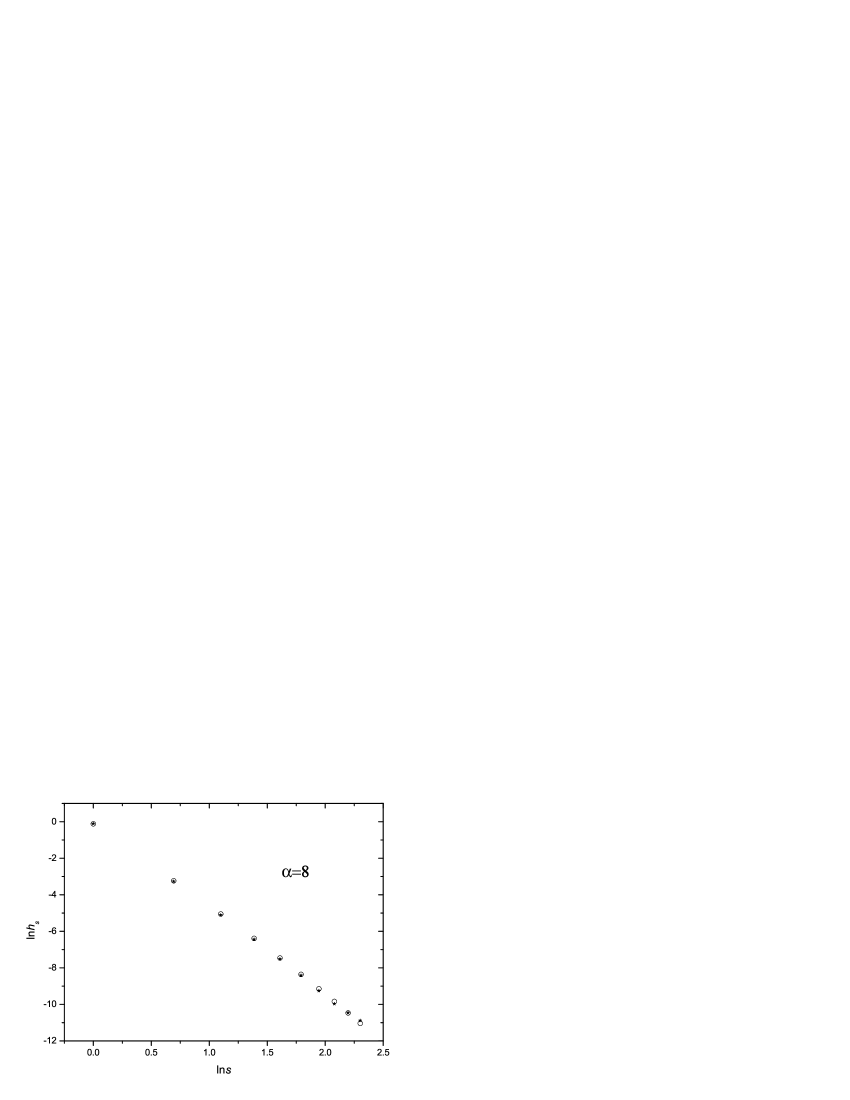
Figure 4: $h_{s}$ for $\alpha=8$ from both numerical calculation and computer simulation. Black stars represent outcome of computer simulation for $N=2.5\times 10^{5}$, $\gamma=2$ and $a=0.88889$. Total $2\times 10^{6}$ time steps were run and the final $5\times 10^{5}$ time steps were used to count $n_{s}$ statistically. The circles represent the theoretical results derived from Eqs.(4-5).

V Discussions

In this paper, we have introduced a so-called money-based model to mimic and study the wealth allocation process. We find for a wide range of parameters, the wealth distribution $n_{s}\sim A/s^{\eta+1}$ with $\eta$ given by Eq.(15) for sufficiently large $s$. The crucial difference between our model and the EZ model is that the dissociative probability $\Gamma_{d}$ of an economic entity, after he/she is picked up, is proportional to $1/s$ in our model. However, the corresponding probability in the EZ model is simply proportional to 1. This difference gives rise to divergent behaviors of $n_{s}$. In the EZ model, $n_{s}\sim A/s^{2.5}\exp(-\alpha s)$ for large $s$ ez2 . When $n_{s}$ is interpreted as the number of individuals who own $s$ units of assets, the choice of $\Gamma_{d}\sim O(1/s)$ is reasonable. Actually, since at the first step, we randomly picked up a unit of money, the individual who owns $s$ units of assets is picked up with a probability proportional to $s$. According to the observation in real economic life, large companies or rich men are often much more robust than small or poor ones when confronting economic impact and fierce competition. If $\Gamma_{d}\sim O(1)$, the overall dissociation frequency would be proportional to $s$ which is totally unreasonable.

In real economic environment, capitals and agents behave similarly at some point. For instance, they both ceaselessly display integration and disintegration, driven by the motivation to maximize profits and efficiency. This mechanism updates the system every time, and gives rise to clusters and herd behaviors. Furthermore, in an agent-based model, it is usually indispensable to consider the individual diversity that is all too often hard to deal with. When it comes to the money-based model, this micro complexity may be considerably simplified. Finally, the conceptual movement and interaction among capitals is not as restricted by space and time as between agents. Therefore, when econophysics is much more interested in the behaviors of capitals than that of agents, it is recommendable to adopt such a money-based model.

The methodology to fix our attention on the capital movements, instead of interactions among individuals, will bring a lot of facility for analysis; moreover, using such random variables as $\gamma$ and $a$ to represent the macro level of the micro mechanism also help us find a possible bridge between the evolution of the system and the protean behaviors of individuals. Whether the bridge is steady or not can only be tested by further investigation.

- (1) G.K.Zipf, Human Behavior and the Principle of Least Effort (Addison-Wesley Press, Cambridge, MA, 1949).
- (2) V. Pareto, Cours d’Economique Politique (Macmillan, Paris, 1897), Vol 2.
- (3) B. Mandelbrot, Economietrica 29,517(1961).
- (4) B.B. Mandelbrot, Comptes Rendus 232, 1638(1951).
- (5) B.B. Mandelbrot, J. Business 36, 394(1963).
- (6) A.B. Atkinson and A.J. Harrison, Distribution of Total Wealth in Britain (Cambridge University Press, Cambridge, 1978).
- (7) H. Takayasu, A.-H. Sato and M. Takayasu, Phys.Rev.Lett. 79,966(1997).
- (8) P.W. Anderson, in The Economy as an Evolving Complex System II, edited by W.B. Arthur, S.N. Durlauf and D.A. Lane (Addison-Wesley, Reading, MA,1997).
- (9) The Theory of Income and Wealth Distribution, edited by Y.S. Brenner et al.,(New York, St. Martin’s Press, 1988).
- (10) H.A. Simon and C.P. Bonini, Am. Econ. Rev. 48,607(1958).
- (11) U.G. Yule, Philos. Tran. R. Soc. London, Ser. Bc213,21(1924).
- (12) D.G. Champernowne, Econometrica 63, 318(1953).
- (13) H. Kesten, Acta Math. 131,207(1973).
- (14) S. Solomon, in Annual Reviews of Computational Physics II, edited by D. Stauffer (World Scientific, Singapore, 1995), p.243.
- (15) M. Levy and S. Solomon, Int. J. Mod. Phys. C 7, 595(1996).
- (16) S. Solomon and M. Levy, Int. J. Mod. Phys. C 7, 745(1996).
- (17) O. Malcai, O. Biham and S. Solomon, Phys. Rev. E 60, 1299(1999).
- (18) B.B. Mandelbrot, Int. Ecomomic Rev. 1, 79(1960).
- (19) E.W. Montroll and M.F. Shlesinger, Nonequilibrium Phenomena II. From Stochastics to Hydrodynamics, edited by J.L. Lebowitz, E.W. Montroll(North-Holland, Amsterdam, 1984).
- (20) D. Sornette and R. Cont, J. Phys. I France 7, 431(1997).
- (21) H. Takayasu and K. Okuyama, Fractals 6(1998).
- (22) Z.A. Melzak, Mathematical Ideas, Modeling and Applications, Volume II of Companion to Concrete Mathematics (Wiley, New York, 1976), p279.
- (23) S. Ispolatov, P.L. Krapivsky and S. Redner, Euro. Phys. J. B 2, 267(1998).
- (24) A. Dragulescu and V.M. Yakovenko, Euro. Phys. J. B 17, 723(2000).
- (25) C.B. Yang, to be published in Chinese Phys. Lett.
- (26) V.M. Eguíluz and M.G. Zimmermann, Phys. Rev. Lett. 85,5659(2000).
- (27) R. D’Hulst and G.J. Rodgers, Euro. Phys. J. B 20,619(2001).
- (28) Y.B. Xie, B.H. Wang, H.J. Quan, W.S. Yang and P.M. Hui, Phys. Rev. E 65, 046130(2002).
- (29) Y.B. Xie, B.H. Wang, H.J. Quan, W.S. Yang and W.N. Wang, Acta Physica Sinica (Chinese), 52,2399(2003).
- (30) B. Hu, Y.B. Xie, T. Zhou and B.H. Wang (unpublished).