Asymmetry and decoherence in a double-layer persistent-current qubit

Abstract

Superconducting circuits fabricated using the widely used shadow evaporation technique can contain unintended junctions which change their quantum dynamics. We discuss a superconducting flux qubit design that exploits the symmetries of a circuit to protect the qubit from unwanted coupling to the noisy environment, in which the unintended junctions can spoil the quantum coherence. We present a theoretical model based on a recently developed circuit theory for superconducting qubits and calculate relaxation and decoherence times that can be compared with existing experiments. Furthermore, the coupling of the qubit to a circuit resonance (plasmon mode) is explained in terms of the asymmetry of the circuit. Finally, possibilities for prolonging the relaxation and decoherence times of the studied superconducting qubit are proposed on the basis of the obtained results.

I Introduction

Superconducting (SC) circuits in the regime where the Josephson energy $E_{J}$ dominates the charging energy $E_{C}$ represent one of the currently studied candidates for a solid-state qubit MSS . Several experiments have demonstrated the quantum coherent behavior of a SC flux qubit Mooij ; Orlando ; vanderWal , and recently, coherent free-induction decay (Ramsey fringe) oscillations have been observed CNHM . The coherence time $T_{2}$ extracted from these data was reported to be around $20\,{\rm ns}$, somewhat shorter than expected from theoretical estimates Devoret ; Tian99 ; Tian02 ; WWHM . In more recent experiments Delft-new , it was found that the decoherence time $T_{2}$ can be increased up to approximately $120\,{\rm ns}$ by applying a large dc bias current (about $80\%$ of the SQUID junctions’ critical current).

A number of decoherence mechanisms can be important, being both intrinsic to the Josephson junctions, e.g., oxide barrier defects Martinis or vortex motion, and external, e.g., current fluctuations from the external control circuits, e.g., current sources Devoret ; Tian99 ; Tian02 ; WWHM ; BKD . Here, we concentrate on the latter effect, i.e., current fluctuations, and use a recently developed circuit theory BKD to analyze the circuit studied in the experiment CNHM .

Figure 1: Schematic of the circuit. Crosses denote Josephson junctions. The outer loop with two junctions $L$ and $R$ forms a dc SQUID that is used to read out the qubit. The state of the qubit is determined by the orientation of the circulating current in the small loop, comprising the junctions $1$, $2$, and $3$, one of which has a slightly smaller critical current than the others. A bias current $I_{B}$ can be applied as indicated for read-out.

The SC circuit studied in Ref. CNHM (see Fig. 1) is designed to be immune to current fluctuations from the current bias line due to its symmetry properties; at zero dc bias, $I_{B}=0$, and independent of the applied magnetic field, a small fluctuating current $\delta I_{B}(t)$ caused by the finite impedance of the external control circuit (the current source) is divided equally into the two arms of the SQUID loop and no net current flows through the three-junction qubit line.

Figure 2: Schematics of Josephson junctions produced by the shadow evaporation technique, connecting the upper with the lower aluminum layer. Shaded regions represent the aluminum oxide.

Thus, in the ideal circuit, Fig. 1, the qubit is protected from decoherence due to current fluctuations in the bias current line. This result also follows from a systematic analysis of the circuit BKD . However, asymmetries in the SQUID loop may spoil the protection of the qubit from decoherence. The breaking of the SQUID’s symmetry has other very interesting consequences, notably the possibility to couple the qubit to an external harmonic oscillator (plasmon mode) and thus to entangle the qubit with another degree of freedom Chiorescu-coupling . For an inductively coupled SQUID Mooij ; Orlando ; vanderWal , a small geometrical asymmetry, i.e., a small imbalance of self-inductances in a SQUID loop combined with the same imbalance for the mutual inductance to the qubit, is not sufficient to cause decoherence at zero bias current BKD . A junction asymmetry, i.e., a difference in critical currents in the SQUID junctions $L$ and $R$, would in principle suffice to cause decoherence at zero bias current. However, in practice, the SQUID junctions are typically large in area and thus their critical currents are rather well-controlled (in the system studied in Ref. Delft-new , the junction asymmetry is $<5\%$), therefore the latter effect turns out to be too small to explain the experimental findings.

An important insight in the understanding of decoherence in the circuit design proposed in CNHM is that it contains another asymmetry, caused by its double layer structure. The double layer structure is an artifact of the fabrication method used to produce SC circuits with aluminum/aluminum oxide Josephson junctions, the so-called shadow evaporation technique. Junctions produced with this technique will always connect the top layer with the bottom layer, see Fig. 2.

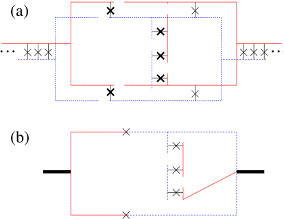
Figure 3: (a) Double layer structure. Dashed blue lines represent the lower, solid red lines the upper SC layer, and crosses indicate Josephson junctions. The thick crosses are the intended junctions, while the thin crosses are the unintended distributed junctions due to the double-layer structure. (b) Simplest circuit model of the double layer structure. The symmetry between the upper and lower arms of the SQUID has been broken by the qubit line comprising three junctions. Thick black lines denote pieces of the SC in which the upper and lower layer are connected by large area junctions.

Thus, while circuits like Fig. 1 can be produced with this technique, strictly speaking, loops will always contain an even number of junctions. In order to analyze the implications of the double layer structure for the circuit in Fig. 1, we draw the circuit again, see Fig. 3(a), but this time with separate upper and lower layers. Every piece of the upper layer will be connected with the underlying piece of the lower layer via an “unintentional” Josephson junction.

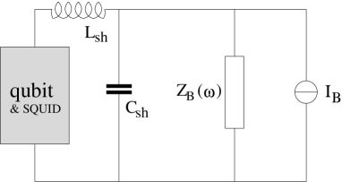
Figure 4: External circuit attached to the qubit (Fig. 1) that allows the application of a bias current $I_{B}$ for qubit read-out. The inductance $L_{\rm sh}$ and capacitance $C_{\rm sh}$ form the shell circuit, and $Z(\omega)$ is the total impedance of the current source ($I_{B}$). The case where a voltage source is used to generate a current can be reduced to this using Norton’s theorem.

However, these extra junctions typically have large areas and therefore large critical currents; thus, their Josephson energy can often be neglected. Since we are only interested in the lowest-order effect of the double layer structure, we neglect all unintentional junctions in this sense; therefore, we arrive at the circuit, Fig. 3(b), without extra junctions. We notice however, that this resulting circuit is distinct from the ’ideal’ circuit Fig. 1 that does not reflect the double-layer structure. In the real circuit, Fig. 3(b), the symmetry between the two arms of the dc SQUID is broken, and thus it can be expected that bias current fluctuations cause decoherence of the qubit at zero dc bias current, $I_{B}=0$. This effect is particularly important in the circuit discussed in CNHM ; Delft-new since the coupling between the qubit and the SQUID is dominated by the kinetic inductance of the shared line, and so is strongly asymmetric, rather than by the geometric mutual inductance vanderWal which is symmetric. Our analysis below will show this quantitatively and will allow us to compare our theoretical predictions with the experimental data for the decoherence times as a function of the bias current. Furthermore, we will theoretically explain the coupling of the qubit to a plasma mode in the read-out circuit (SQUID plus external circut), see Fig. 4, at $I_{B}=0$; this coupling is absent for a symmetric circuit.

This article is organized as follows. In Sec. II, we derive the Hamiltonian of the qubit, taking into account its double-layer structure. We use this Hamiltonian to calculate the relaxation and decoherence times as a function of the applied bias current (Sec. III) and to derive an effective Hamiltonian for the coupling of the qubit to a plasmon mode in the read-out circuit (Sec. IV). Finally, Sec. V contains a short discussion of our result and possible lessons for future SC qubit designs.

II Hamiltonian

In order to model the decoherence of the qubit, we need to find its Hamiltonian and its coupling to the environment. The Hamiltonian of the circuit Fig. 3(b) can be found using the circuit theory developed in Ref. BKD . To this end, we first draw the circuit graph (Fig. 5) and find a tree of the circuit graph containing all capacitors and as few inductors as possible (Fig. 6). A tree of a graph is a subgraph containing all of its nodes but no loops. By identifying the fundamental loops BKD in the circuit graph (Fig. 5) we obtain the loop submatrices

$${\bf F}_{CL}=\left(\begin{array}[]{r r}-1&1\cr-1&1\cr-1&1\cr 0&-1\cr 0&-1\end{array}\right), {\bf F}_{CZ}=-{\bf F}_{CB}=\left(\begin{array}[]{r}0\cr 0\cr 0\cr 1\cr 0\end{array}\right),$$ (11)

$${\bf F}_{KL}=\left(\begin{array}[]{r r}0&-1\cr 0&-1\cr-1&1\end{array}\right), {\bf F}_{KZ}=-{\bf F}_{KB}=\left(\begin{array}[]{r}1\cr 1\cr 0\end{array}\right).$$ (18)

The chord ($L$) and tree ($K$) inductance matrices are taken to be

$${\bf L}=\left(\begin{array}[]{c c}L/2&M/4\\ M/4&L^{\prime}/2\end{array}\right),\quad\quad{\bf L}_{K}=\left(\begin{array}[]{c c c}L/2&M/4&M_{i}\\ M/4&L^{\prime}/2&0\\ M_{i}&0&L_{i}\end{array}\right),$$ (19)

where $L$, $L^{\prime}$, and $L_{i}$ are, respectively, the self-inductances of the qubit loop in the upper layer, the SQUID, and qubit loop in the lower layer, and $M$ and $M_{i}$ are the mutual inductances between the qubit and the SQUID and between the upper and lower layers in the qubit loop. The tree-chord mutual inductance matrix is taken to be

$${\bf L}_{LK}=\left(\begin{array}[]{c c c}0&M/4&0\\ M/4&0&0\end{array}\right).$$ (20)

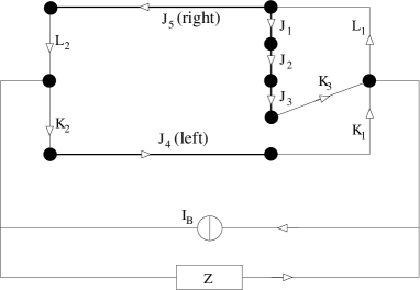
Figure 5: The network graph of the circuit, Figs. 3b and 4. Dots indicate the nodes, lines the branches of the graph; an arrow indicates the orientation of a branch. Thick lines labeled $J_{i}$ denote an RSJ element, i.e., a Josephson junction shunted by a capacitor and a resistor. Lines labeled $L_{i}$ and $K_{i}$ denote inductances, $Z_{\rm ext}$ the external impedance, including the shell circuit of Fig. 4, and $I_{B}$ is the current source.

The Hamiltonian in terms of the SC phase differences ${\mbox{\boldmath$\varphi$}}=(\varphi_{1},\varphi_{2},\varphi_{3},\varphi_{L},\varphi_{R})$ across the Josephson junctions and their conjugate variables, the capacitor charges ${\bf Q}_{C}$, is found to be BKD

$${\cal H}_{S}=\frac{1}{2}{\bf Q}_{C}^{T}{\bf C}^{-1}{\bf Q}_{C}+\left(\frac{\Phi_{0}}{2\pi}\right)^{2}U({\mbox{\boldmath$\varphi$}}),$$ (21)

with the potential

$$U({\mbox{\boldmath$\varphi$}}) = -\sum_{i}\frac{1}{L_{J;i}}\cos\varphi_{i}+\frac{1}{2L_{Q}}\left(\varphi_{1}+\varphi_{2}+\varphi_{3}-f\right)^{2}$$

$$+ \frac{1}{2L_{S}}\left(\varphi_{L}+\varphi_{R}-f^{\prime}\right)^{2}$$

$$+ \frac{1}{M_{QS}}\left(\varphi_{1}+\varphi_{2}+\varphi_{3}-f\right)\left(\varphi_{L}+\varphi_{R}-f^{\prime}\right)$$

$$+ \frac{2\pi}{\Phi_{0}}I_{B}\left[m_{Q}\left(\varphi_{1}+\varphi_{2}+\varphi_{3}\right)+m_{L}\varphi_{L}+m_{R}\varphi_{R}\right],$$

where the Josephson inductances are given by $L_{J;i}=\Phi_{0}/2\pi I_{c;i}$, and $I_{c;i}$ is the critical current of the $i$-th junction. In Eq. (II), we have also introduced the effective self-inductances of the qubit and SQUID and the effective qubit-SQUID mutual inductance,

$$L_{Q} = L\frac{\kappa}{4(1+L^{\prime}/L+2M/L)},$$ (23)

$$L_{S} = L\frac{\kappa}{2(1+2L_{i}/L)},$$ (24)

$$M_{QS} = -L\frac{\kappa}{2(1+M/L+2M_{i}/L)},$$ (25)

and the coupling constants between the bias current and the qubit and the left and right SQUID phases,

$$m_{Q} = \kappa^{-1}(1+L^{\prime}/L+2M/L)(1-2M_{i}/L),$$ (26)

$$m_{L} = \frac{1}{2}-\frac{1}{2\delta},\quad\quad m_{R}=-\frac{1}{2}-\frac{1}{2\delta},$$ (27)

with the definitions

$$\kappa = 1+4L_{i}(L+L^{\prime}+2M)/L^{2}+2(L^{\prime}+M-2M_{i})/L$$ (28)

$$-(M+2M_{i})^{2}/L^{2},$$

$$\delta = \kappa/(1+M/L+2M_{i}/L)(1-2M_{i}/L).$$ (29)

The sum $\varphi_{1}+\varphi_{2}+\varphi_{3}$ is the total phase difference across the qubit line containing junctions $J_{1}$, $J_{2}$, and $J_{3}$, whereas $\varphi_{L}+\varphi_{R}$ is the sum of the phase differences in the SQUID loop. Furthermore, ${\bf C}={\rm diag}(C,C,C,C^{\prime},C^{\prime})$ is the capacitance matrix, $C$ and $C^{\prime}$ being the capacitances of the qubit and SQUID junctions, respectively.

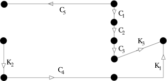
Figure 6: A tree of the circuit graph, Fig. 5. A tree is a subgraph connecting all nodes, containing no loops. Here, the tree was chosen to contain all capacitors $C_{i}$ (from the RSJ elements) and as few inductors $K_{i}$ as possible (see Ref. BKD ).

The working point is given by the triple $(f,f^{\prime},I_{B})$, i.e., by the bias current $I_{B}$, and by the dimensionless external magnetic fluxes threading the qubit and SQUID loops, $f=2\pi\Phi_{x}/\Phi_{0}$ and $f^{\prime}=2\pi\Phi_{x}^{\prime}/\Phi_{0}$. We will work in a region of parameter space where the potential $U({\mbox{\boldmath$\varphi$}})$ has a double-well shape, which will be used to encode the logical qubit states $|0\rangle$ and $|1\rangle$.

The classical equations of motion, including dissipation, are

$${\bf C}\ddot{\mbox{\boldmath$\varphi$}}=-\frac{\partial U}{\partial{\mbox{\boldmath$\varphi$}}}-\mu K*{\bf m}({\bf m}\cdot{\mbox{\boldmath$\varphi$}}),$$ (30)

where convolution is defined as $(f*g)(t)=\int_{-\infty}^{t}f(t-\tau)g(\tau)d\tau$. The vector ${\bf m}$ is given by

$${\bf m}=A(m_{Q},m_{Q},m_{Q},m_{L},m_{R}),$$ (31)

and $A$ is chosen such that $|{\bf m}|=1$. For the coupling constant $\mu$, we find

$$\mu = \kappa^{-2}L^{-4}\left(3\,{\left({L}+{L^{\prime}}+2\,M\right)}^{2}\,{\left({L}+M-2\,{M_{i}}\right)}^{2}\right.$$

$$\left.+\left(2\,{L_{i}}\,\left({L}+{L^{\prime}}+2\,M\right)+{L}\,\left({L^{\prime}}-2\,{M_{i}}\right)\right.\right.$$

$$\left.\left.-M\,\left(M+2\,{M_{i}}\right)\right)^{2}+\left({{L}}^{2}+2\,{L_{i}}\,\left({L}+{L^{\prime}}+2\,M\right)\right.\right.$$

$$\left.\left.+{L}\,\left({L^{\prime}}+2\,M-2\,{M_{i}}\right)-2\,{M_{i}}\,\left(M+2\,{M_{i}}\right)\right)^{2}\right).$$

The kernel $K$ in the dissipative term is determined by the total external impedance; in the frequency domain,

$$K(\omega)=\frac{i\omega}{Z(\omega)},$$ (33)

with the impedance

$$Z(\omega)=Z_{\rm ext}(\omega)+i\omega L_{\rm int},$$ (34)

where we have defined the internal inductance,

$$L_{\rm int} = \frac{1}{4\kappa L^{2}}\left(4L_{i}(L+L^{\prime})(L+L^{\prime}+2M)+2L^{2}L^{\prime}\right.$$

$$-LM^{2}-4L^{\prime}MM_{i}-8L^{\prime}M_{i}^{2}-8MM_{i}^{2}$$

$$\left.+L(2L^{\prime 2}+2L^{\prime}M-M^{2}+4MM_{i}-8M_{i}^{2})\right),$$

and where

$$Z_{\rm ext}=\left(\frac{1}{Z_{B}(\omega)}+i\omega C_{\rm sh}\right)^{-1}+i\omega L_{\rm sh}$$ (36)

is the impedance of the external circuit attached to the qubit, including the shell circuit, see Figs. 4,5. For the parameter regime we are interested in, $L_{\rm int}\approx 20\,{\rm pH}$, $\omega\lesssim 10\,{\rm GHz}$, and $Z\gtrsim 50\,\Omega$ therefore $\omega L_{\rm int}\ll|Z_{\rm ext}|$, and we can use $Z(\omega)\approx Z_{\rm ext}(\omega)$.

We numerically find the double-well minima ${\mbox{\boldmath$\varphi$}}_{0}$ and ${\mbox{\boldmath$\varphi$}}_{1}$ for a range of bias currents between $0$ and $4\,\mu{\rm A}$ and external flux $f^{\prime}/2\pi$ between $1.33$ and $1.35$ and a qubit flux around $f/2\pi\simeq 0.5$ (the ratio $f/f^{\prime}=0.395$ is fixed by the areas of the SQUID and qubit loops in the circuit). The states localized at ${\mbox{\boldmath$\varphi$}}_{0}$ and ${\mbox{\boldmath$\varphi$}}_{1}$ are encoding the logical $|0\rangle$ and $|1\rangle$ states of the qubit. This allows us to find the set of parameters for which the double well is symmetric, $\epsilon\equiv U({\mbox{\boldmath$\varphi$}}_{0})-U({\mbox{\boldmath$\varphi$}}_{1})=0$. The curve $f^{*}(I_{B})$ on which the double well is symmetric is plotted in Fig. 7. Qualitatively, $f^{*}(I_{B})$ agrees well with the experimentally measured symmetry line Delft-new , but it underestimates the magnitude of the variation in flux $f^{\prime}$ as a function of $I_{B}$. The value of $I_{B}$ where the symmetric and the decoupling lines intersect coincides with the maximum of the symmetric line, as can be understood from the following argument. Taking the total derivative with respect to $I_{B}$ of the relation $\epsilon=U({\mbox{\boldmath$\varphi$}}_{0};f^{*}(I_{B}),I_{B})-U({\mbox{\boldmath$\varphi$}}_{1};f^{*}(I_{B}),I_{B})=0$ on the symmetric line, and using that ${\mbox{\boldmath$\varphi$}}_{0,1}$ are extremal points of $U$, we obtain ${\bf n}\cdot\Delta{\mbox{\boldmath$\varphi$}}\,\partial f^{*}/\partial I_{B}+(2\pi/\Phi_{0}){\bf m}\cdot\Delta{\mbox{\boldmath$\varphi$}}=0$ for some constant vector ${\bf n}$. Therefore, ${\bf m}\cdot\Delta{\mbox{\boldmath$\varphi$}}=0$ (decoupling line) and ${\bf n}\cdot\Delta{\mbox{\boldmath$\varphi$}}\neq 0$ implies $\partial f^{*}/\partial I_{B}=0$.

For the numerical calculations throughout this paper, we use the estimated experimental parameters from Delft-new ; Chiorescu-coupling , $L=25\,{\rm pH}$, $L^{\prime}=45\,{\rm pH}$, $M=7.5\,{\rm pH}$, $L_{i}=10\,{\rm pH}$, $M_{i}=4\,{\rm pH}$, $I_{c;L}=I_{c;R}=4.2\,\mu{\rm A}$, and $I_{c;1}=I_{c;2}/\alpha=I_{c;3}=0.5\,\mu{\rm A}$ with $\alpha\simeq 0.8$.

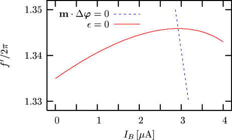
Figure 7: Decoupling (red solid) and symmetric (blue dashed) curves in the $(I_{B},f^{\prime})$ plane, where $I_{B}$ is the applied bias current and $f^{\prime}=2\pi\Phi_{x}^{\prime}/\Phi_{0}$ is the dimensionless externally applied magnetic flux threading the SQUID loop. Both curves are obtained from the numerical minimization of the potential Eq. (II). The decoupling line is determined using the condition ${\bf m}\cdot\Delta{\mbox{\boldmath$\varphi$}}=0$, whereas the symmetric line follows from the condiction $\epsilon=0$.

III Decoherence

The dissipative quantum dynamics of the qubit will be described using a Caldeira-Leggett model CaldeiraLeggett which is consistent with the classical dissipative equation of motion, Eq. (30). We then quantize the combined system and bath Hamiltonian and use the master equation for the superconducting phases $\varphi$ of the qubit and SQUID in the Born-Markov approximation to obtain the relaxation and decoherence times of the qubit.

III.1 Relaxation time $T_{1}$

The relaxation time of the qubit in the semiclassical approximation fn1 is given by

$$T_{1}^{-1}=\frac{\Delta^{2}}{E^{2}}\left(\frac{\Phi_{0}}{2\pi}\right)^{2}|{\bf m}\cdot\Delta{\mbox{\boldmath$\varphi$}}|^{2}{\rm Re}\frac{E}{Z(E)}\coth\left(\frac{E}{2k_{B}T}\right),$$ (37)

where $\Delta{\mbox{\boldmath$\varphi$}}\equiv{\mbox{\boldmath$\varphi$}}_{0}-{\mbox{\boldmath$\varphi$}}_{1}$ is the vector joining the two minima in configuration space and

$$E=\sqrt{\Delta^{2}+\epsilon^{2}}$$ (38)

is the energy splitting between the two (lowest) eigenstates of the double well and $\Delta$ is the tunnel coupling between the two minima. We will evaluate $T_{1}$ on the symmetric line where $\epsilon=0$, and therefore, $E=\Delta$. At the points in parameter space $(I_{B},f^{\prime})$ where ${\bf m}\cdot\Delta{\mbox{\boldmath$\varphi$}}$ vanishes, the system will be decoupled from the environment (in lowest order perturbation theory), and thus $T_{1}\rightarrow\infty$. From our numerical determination of ${\mbox{\boldmath$\varphi$}}_{0}$ and ${\mbox{\boldmath$\varphi$}}_{1}$, the decoupling flux $f^{\prime}$, at which ${\bf m}\cdot\Delta{\mbox{\boldmath$\varphi$}}=0$, is obtained as a function of $I_{B}$ (Fig. 7). From this analysis, we can infer the parameters $(I_{B},f^{\prime})$ at which $T_{1}$ will be maximal and the relaxation time away from the divergence. In practice, the divergence will be cut off by other effects which lie beyond the scope of this theory. However, we can fit the peak value of $T_{1}$ from recent experiments Delft-new with a residual impedance of $R_{\rm res}\simeq 3.5\,{\rm M}\Omega$ which lies in a different part of the circuit than $Z$ (Fig.5). We do not need to further specify the position of $R_{\rm res}$ in the circuit; we only make use of the fact that it gives rise to an additional contribution to the relaxation rate of the form Eq. (37) but with a vector ${\bf m}_{\rm res}\neq{\bf m}$, with ${\bf m}_{\rm res}\cdot\Delta{\mbox{\boldmath$\varphi$}}\neq 0$ on the decoupling line. Without loss of generality, we can adjust $R_{\rm res}$ such that ${\bf m}_{\rm res}\cdot\Delta{\mbox{\boldmath$\varphi$}}=1$. Such a residual coupling may, e.g., originate from the subgap resistances of the junctions. The relaxation time $T_{1}$ obtained from Eq. (37) as a function of $I_{B}$ along the symmetric line $\epsilon=0$ (Fig. 7) with a cut-off of the divergence by $R_{\rm res}$ is plotted in Fig. 8, along with the experimental data from sample A in Delft-new . In Fig. 9, we also plot $T_{1}$ (theory and experiment) as a function of the applied magnetic flux around the symmetric point at zero bias current. For the plots of $T_{1}$ in Figs. 8 and 9, we have used the experimental parameters $\Delta/h=5.9\,{\rm GHz}$, $Z(E)\simeq Z_{\rm ext}(E)=60\,\Omega$, and $T=100\,{\rm mK}$.

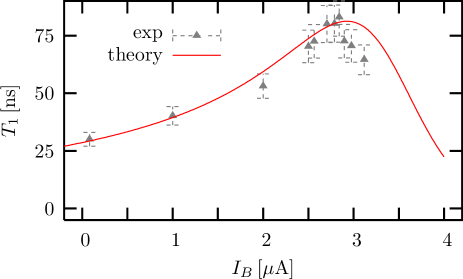
Figure 8: Theoretical relaxation time $T_{1}$ (solid line) as a function of the applied bias current $I_{B}$, along the symmetric line (Fig. 7). The value of $I_{B}$ where $T_{1}$ diverges coincides with the intersection of the symmetric line with the decoupling line in Fig. 7; the divergence is removed in the theory curve by including a residual impedance of $R_{\rm res}=3.5\,{\rm M}\Omega$. The experimentally obtained data for sample A in Ref. Delft-new, are shown as triangle symbols with error bars.

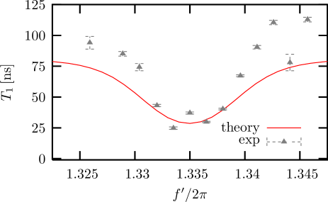
Figure 9: Theoretical relaxation time $T_{1}$ (solid line) as a function of the applied magnetic flux $f^{\prime}=\Phi_{x}^{\prime}/\Phi_{0}$ at zero bias current, $I_{B}=0$, around the symmetric point, $\epsilon=0$. Experimentally obtained data for sample A in Ref. Delft-new, are shown as triangle symbols with error bars. The theory curve from the semiclassical $T_{1}$ formula, Eq. (37), is expected to be valid in the range $|\epsilon|\lesssim\Delta$, which corresponds roughly to $1.33\lesssim f^{\prime}/2\pi\lesssim 1.34$. Experimental points outside the plotted range of $f^{\prime}$ where the theory curve is not expected to be valid, are not shown.

III.2 Decoherence time $T_{2}$

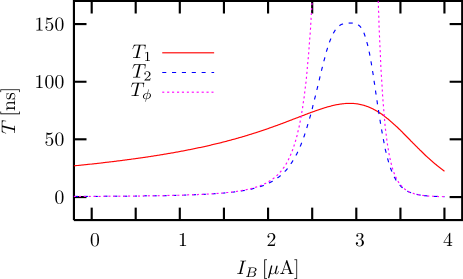
Figure 10: Theoretical relaxation, pure dephasing, and decoherence times $T_{1}$, $T_{\phi}$, and $T_{2}$ as a function of applied bias current $I_{B}$, along the symmetric line (Fig. 7). As in Fig. 8, we have included decoherence from a residual impedance of $R_{\rm res}=3.5\,{\rm M}\Omega$.

The decoherence time $T_{2}$ is related to the relaxation time $T_{1}$ via

$$\frac{1}{T_{2}}=\frac{1}{T_{\phi}}+\frac{1}{2T_{1}},$$ (39)

where $T_{\phi}$ denotes the (pure) dephasing time. On the symmetric line $f^{\prime}=f^{*}(I_{B})$ (see Fig. 7), the contribution to the dephasing rate $T_{\phi}^{-1}$ of order $R_{Q}/Z$ vanishes, where $R_{Q}=e^{2}/h\approx 25.8\,{\rm k}\Omega$ denotes the quantum of resistance. However, there is a second-order contribution $\propto(R_{Q}/Z)^{2}$, which we can estimate as follows. The asymmetry $\epsilon=U({\mbox{\boldmath$\varphi$}}_{0})-U({\mbox{\boldmath$\varphi$}}_{1})$ of the double well as a function of the bias current $I_{B}$ at fixed external flux $f^{\prime}$ can be written in terms of a Taylor series around $I_{B}^{*}$,

$$\epsilon(I_{B})=\epsilon_{0}+\epsilon_{1}\delta I_{B}+\epsilon_{2}\delta I_{B}^{2}+O(\delta I_{B})^{3},$$ (40)

where $\delta I_{B}(t)=I_{B}(t)-I_{B}^{*}$ is the variation away from the dc bias current $I_{B}^{*}$. The coefficients $\epsilon_{i}(I_{B})$ can be obtained numerically from the minimization of the potential $U$, Eq. (II). The approximate two-level Hamiltonian $\frac{\Delta}{2}\sigma_{X}+\frac{\epsilon}{2}\sigma_{Z}$ in its eigenbasis is then, up to $O(\delta I_{B}^{3})$,

$$H = \frac{1}{2}\sqrt{\Delta^{2}+\epsilon^{2}}\sigma_{z}=\frac{\Delta}{2}\sigma_{z}+\frac{\epsilon^{2}}{4\Delta}\sigma_{z}$$ (41)

$$= \frac{\tilde{\Delta}}{2}\sigma_{z}+\frac{\epsilon_{0}\epsilon_{1}}{2\Delta}\sigma_{z}\delta I_{B}+\left(\frac{\epsilon_{1}^{2}}{4\Delta}+\frac{\epsilon_{0}\epsilon_{2}}{2\Delta}\right)\sigma_{z}\delta I_{B}^{2},\quad$$ (42)

where $\tilde{\Delta}=\Delta+\epsilon_{0}^{2}/2\Delta$. On the symmetric line, $\epsilon_{0}=0$, the term linear in $\delta I_{B}$ vanishes. However, there is a non-vanishing second-order term $\propto\epsilon_{1}^{2}$ that contributes to dephasing on the symmetric line. Without making use of the correlators for $\delta I_{B}^{2}$, we know that the pure dephasing rate $T_{\phi}^{-1}$ will be proportional to $\epsilon_{1}(I_{B})^{4}$ which allows us to predict the dependence of $T_{\phi}$ on $I_{B}$. A discussion of the second-order dephasing within the spin-boson model can be found in MakhlinShnirman . However, in order to explain the order of magnitude of the experimental result Delft-new for $T_{\phi}$ correctly, the strong coupling to the plasma mode may also play an important role Delft-new ; Bertet-unpublished . The result presented here cannot be used to predict the absolute magnitude of $T_{\phi}$, but we can obtain an estimate for the dependence of $T_{\phi}$ on the bias current $I_{B}$ via $\epsilon_{1}(I_{B})=d\epsilon/dI_{B}$ obtained numerically from our circuit theory, via

$$T_{\phi}^{-1}(I_{B})\approx T_{\phi}^{-1}(0)\left(\frac{\epsilon_{1}(I_{B})}{\epsilon_{1}(0)}\right)^{4},$$ (43)

where for dimensional reasons we can write the proportionality constant in terms of a zero-frequency resistance $R_{0}$ and an energy $\bar{\omega}$ (note, however, that this corresponds to one free parameter in the theory), $T_{\phi}^{-1}(0)/\epsilon_{1}(0)\approx 2\bar{\omega}^{3}/R_{0}^{2}\Delta^{2}$. For the plots of $T_{\phi}$ and $T_{2}$ in Fig. 10, we have used the resistance $R_{0}=1450\,\Omega$ and have chosen $\bar{\omega}/2\pi\approx 1\,{\rm THz}$ to approximately fit the width of the $T_{2}$ curve. The relaxation, dephasing, and decoherence times $T_{1}$, $T_{\phi}$, and $T_{2}$ are plotted as a function of the bias current $I_{B}$ in Fig. 8 and Fig. 10.

The calculated relaxation and decoherence times $T_{1}$ and $T_{2}$ agree well with the experimental data Delft-new in their most important feature, the peak at $I_{B}\approx 2.8\,\mu{\rm A}$. This theoretical result does not involve fitting with any free parameters, since it follows exclusively from the independently known values for the circuit inductances and critical currents. Moreover, we obtain good quantitative agreement between theory and experiment for $T_{1}$ away from the divergence. The shape of the $T_{1}$ and $T_{2}$ curves can be understood qualitatively from the theory.

IV Coupling to the plasmon mode

In addition to decoherence, the coupling to the external circuit (Fig. 4) can also lead to resonances in the microwave spectrum of the system that originate from the coupling between the qubit to a LC resonator formed by the SQUID, the inductance $L_{\rm sh}$ and capacitance $C_{\rm sh}$ of the “shell” circuit (plasmon mode). We have studied this coupling quantitatively in the framework of the circuit theory BKD , by replacing the circuit elements $I_{B}$ and $Z$ in the circuit graph by the elements $L_{\rm sh}$ and $C_{\rm sh}$ in series, obtaining the graph matrices

$${\bf F}_{CL}=\left(\begin{array}[]{r r r}-1&1&0\cr-1&1&0\cr-1&1&0\cr 0&-1&1\cr 0&-1&0\cr 0&0&-1\end{array}\right)\!\!,\,{\bf F}_{KL}=\left(\begin{array}[]{r r r}0&-1&1\cr 0&-1&1\cr-1&1&0\end{array}\right)\!,$$ (53)

where the last row in ${\bf F}_{CL}$ corresponds to the tree branch $C_{\rm sh}$ and the rightmost column in both ${\bf F}_{CL}$ and ${\bf F}_{KL}$ correspond to the loop closed by the chord $L_{\rm sh}$.

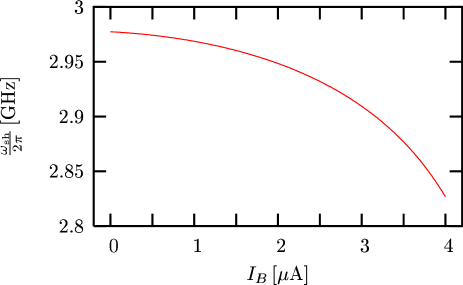
Figure 11: Plasma frequency $\omega_{\rm sh}$ as a function of the applied bias current $I_{B}$. The variation is due to the change the effective in Josephson inductances as $I_{B}$ is varied.

Neglecting decoherence, the total Hamiltonian can be written as

$${\cal H}={\cal H}_{S}+{\cal H}_{\rm sh}+{\cal H}_{S,{\rm sh}},$$ (54)

where ${\cal H}_{S}$, defined in Eq. (21), describes the qubit and SQUID system. The Hamiltonian of the plasmon mode can be brought into the second quantized form

$${\cal H}_{\rm sh}=\frac{Q_{\rm sh}^{2}}{2C_{\rm sh}}+\left(\frac{\Phi_{0}}{2\pi}\right)^{2}\frac{\varphi_{\rm sh}^{2}}{2L_{\rm t}}=\hbar\omega_{\rm sh}\left(b^{\dagger}b+\frac{1}{2}\right),$$ (55)

by introducing the resonance frequency $\omega_{\rm sh}=1/\sqrt{L_{t}C_{\rm sh}}$, the total inductance (where the SQUID junctions have been linearized at the operating point) $L_{t}\simeq L_{\rm sh}+L^{\prime}/4+L_{J}^{\prime}/(\cos(\varphi_{L})+\cos(\varphi_{R}))$, and the creation and annihilation operators $b^{\dagger}$ and $b$, via

$$\varphi_{\rm sh}=\frac{2\pi}{\Phi_{0}}\sqrt{\frac{\hbar}{2C_{\rm sh}\omega_{\rm sh}}}(b+b^{\dagger})=2\sqrt{\pi}\sqrt{\frac{Z_{\rm sh}}{R_{Q}}}(b+b^{\dagger}),$$ (56)

with the impedance $Z_{\rm sh}=\sqrt{L_{t}/C_{\rm sh}}$. For the coupling between the qubit/SQUID system (the phases $\varphi$) and the plasmon mode (the phase $\varphi_{\rm sh}$ associated with the charge on $C_{\rm sh}$, $Q_{\rm sh}=C_{\rm sh}\Phi_{0}\dot{\varphi}_{\rm sh}/2\pi$, we obtain

$${\cal H}_{S,{\rm sh}}=\left(\frac{\Phi_{0}}{2\pi}\right)^{2}\frac{1}{M_{\rm sh}}\varphi_{\rm sh}{\bf m}\cdot{\mbox{\boldmath$\varphi$}},$$ (57)

where ${\bf m}$ is given in Eq. (31) and $M_{\rm sh}\approx L_{\rm sh}+L^{\prime}/4$ (the exact expression for $M_{\rm sh}$ is a rational function of $L_{\rm sh}$ and the circuit inductances which we will not display here). Using Eq. (56) and the semiclassical approximation

$${\bf m}\cdot{\mbox{\boldmath$\varphi$}}\approx-\frac{1}{2}\sigma_{z}{\bf m}\cdot\Delta{\mbox{\boldmath$\varphi$}}+{\rm const.},$$ (58)

we arrive at

$${\cal H}_{S,{\rm sh}}=\lambda\sigma_{z}(b+b^{\dagger}),$$ (59)

with the coupling strength

$$\lambda=-\sqrt{\pi}\left(\frac{\Phi_{0}}{2\pi}\right)^{2}\sqrt{\frac{Z_{\rm sh}}{R_{Q}}}\frac{1}{M_{\rm sh}}{\bf m}\cdot\Delta{\mbox{\boldmath$\varphi$}}.$$ (60)

Note that this coupling vanishes along the decoupling line (Fig. 7) and also rapidly with the increase of $L_{\rm sh}$.

The complete two-level Hamiltonian then has the well-known Jaynes-Cummings form,

$${\cal H}=\Delta\sigma_{x}+\epsilon\sigma_{z}+\hbar\omega_{\rm sh}\left(b^{\dagger}b+\frac{1}{2}\right)+\lambda\sigma_{z}(b+b^{\dagger}).$$ (61)

For the parameters in Ref. Delft-new, , $C_{\rm sh}=12\,{\rm pF}$ and $L_{\rm sh}=170\,{\rm pH}$, we find $\omega_{\rm sh}\approx 2\pi\times 2.9\,{\rm GHz}$ (see Fig. 11) and $Z_{\rm sh}=5\,\Omega$, thus $\sqrt{Z_{\rm sh}/R_{Q}}\approx 0.01$. Note that the dependence of the Josephson inductance (and thus of $L_{t}$ and $\omega_{\rm sh}$) on the state of the qubit leads to an ac Stark shift term $\propto\sigma_{z}b^{\dagger}b$ which was neglected in the coupling Hamiltonian Eq. (61).

We find a coupling constant of $\lambda\approx 210\,{\rm MHz}$ at $I_{B}=0$. The coupling constant as a function of the bias current $I_{B}$ is plotted in Fig. 12. The relatively high values of $\lambda$ should allow the study of the coupled dynamics of the qubit and the plasmon mode. In particular, recently observed side resonances with the sum and difference frequencies $E\pm\omega_{\rm sh}$ Chiorescu-coupling can be explained in terms of the coupled dynamics, Eq. (61). Also, it should be possible to tune in-situ the coupling to the plasmon mode $\lambda$ at will, using pulsed bias currents.

Figure 12: Coupling constant $\lambda$ between the qubit and the plasmon mode. The coupling disappears at the crossing with the decoupling line (Fig. 7), i.e., when ${\bf m}\cdot\Delta{\mbox{\boldmath$\varphi$}}=0$.

V Discussion

We have found that the double-layer structure of SC circuits fabricated using the shadow evaporation technique can drastically change the quantum dynamics of the circuit due to the presence of unintended junctions. In particular, the double-layer structure breaks the symmetry of the Delft qubit CNHM (see Fig. 1), and leads to relaxation and decoherence. We explain theoretically the observed compensation of the asymmetry at high $I_{B}$ Delft-new and calculate the relaxation and decoherence times $T_{1}$ and $T_{2}$ of the qubit, plotted in Fig. 10. We find good quantitative agreement between theory and experiment in the value of the decoupling current $I_{B}$ where the relaxation and decoherence times $T_{1}$ and $T_{2}$ reach their maximum. In future qubit designs, the asymmetry can be avoided by adding a fourth junction in series with the three qubit junctions. It has already been demonstrated that this leads to a shift of the maxima of $T_{1}$ and $T_{2}$ close to $I_{B}=0$, as theoretically expected, and to an increase of the maximal values of $T_{1}$ and $T_{2}$ Delft-new .

The asymmetry of the circuit also gives rise to an interesting coupling between the qubit and an LC resonance in the external circuit (plasmon mode), which has been observed experimentally Chiorescu-coupling , and which we have explained theoretically. The coupling could potentially lead to interesting effects, e.g., Rabi oscillations or entanglement between the qubit and the plasmon mode.

References

• (1) Y. Makhlin, G. Schön, and A. Shnirman, Rev. Mod. Phys. 73, 357 (2001).
• (2) J. E. Mooij, T. P. Orlando, L. Levitov, L. Tian, C. H. van der Wal, S. Lloyd, Science 285, 1036 (1999).
• (3) T. P. Orlando, J. E. Mooij, L. Tian, C. H. van der Wal, L. S. Levitov, S. Lloyd, J. J. Mazo, Phys. Rev. B 60, 15398 (1999).
• (4) C. H. van der Wal, A. C. J. ter Har, F. K. Wilhelm, R. N. Schouten, C. J. P. M. Harmans, T. P. Orlando, S. Lloyd, and J. E. Mooij, Science 290, 773 (2000).
• (5) I. Chiorescu, Y. Nakamura, C. J. P. M. Harmans, and J. E. Mooij, Science 299, 1869 (2003).
• (6) M. H. Devoret, p. 351 in Quantum fluctuations, lecture notes of the 1995 Les Houches summer school, eds. S. Reynaud, E. Giacobino, and J. Zinn-Justin (Elsevier, The Netherlands, 1997).
• (7) L. Tian, L. S. Levitov, J. E. Mooij, T. P. Orlando, C. H. van der Wal, S. Lloyd, in Quantum Mesoscopic Phenomena and Mesoscopic Devices in Microelectronics, I. O. Kulik, R. Ellialtioglu, eds. (Kluwer, Dordrecht, 2000), pp. 429-438; cond-mat/9910062.
• (8) L. Tian, S. Lloyd, and T. P. Orlando, Phys. Rev. B 65, 144516 (2002).
• (9) C. H. van der Wal, F. K. Wilhelm, C. J. P. M. Harmans, and J. E. Mooij, Eur. Phys. J. B 31, 111 (2003).
• (10) P. Bertet, I. Chiorescu, G. Burkard, K. Semba, C. J. P. M. Harmans, D. P. DiVincenzo, J. E. Mooij, submitted to Phys. Rev. Lett. (cond-mat/0412485).
• (11) R. W. Simmonds, K. M. Lang, D. A. Hite, D. P. Pappas, and J. M. Martinis, Phys. Rev. Lett. 93, 077003 (2004).
• (12) G. Burkard, R. H. Koch, and D. P. DiVincenzo, Phys. Rev. B 69, 064503 (2004).
• (13) I. Chiorescu, P. Bertet, K. Semba, Y. Nakamura, C. J. P. M. Harmans, and J. E. Mooij, Nature 431, 159 (2004).
• (14) A. O. Caldeira and A. J. Leggett, Ann. Phys. (N.Y.) 143, 374 (1983).
• (15) The semiclassical approximation accurately describes the double well in the case where the states centered at the left and right minima are well localized (see Ref. BKD, , Sec. XIA).
• (16) Y. Makhlin and A. Shnirman, Phys. Rev. Lett. 92, 178301 (2004).
• (17) P. Bertet, unpublished.