Self-Organized Criticality and Stock Market Dynamics: an Empirical Study.

Abstract

The Stock Market is a complex self-interacting system, characterized by intermittent behaviour. Periods of high activity alternate with periods of relative calm. In the present work we investigate empirically the possibility that the market is in a self-organized critical state (SOC). A wavelet transform method is used in order to separate high activity periods, related to the avalanches found in sandpile models, from quiescent. A statistical analysis of the filtered data shows a power law behaviour in the avalanche size, duration and laminar times. The memory process, implied by the power law distribution of the laminar times, is not consistent with classical conservative models for self-organized criticality. We argue that a “near-SOC” state or a time dependence in the driver, which may be chaotic, can explain this behaviour.

1 Introduction

Since the publication of the articles of Bak, Tang and Wiesenfeld (BTW) [1], the concept of self-organized criticality (SOC) has been invoked to explain the dynamical behaviour of many complex systems, from physics to biology and the social sciences [2, 3]. The key concept of SOC is that complex systems, that is systems constituted by many interacting elements, although obeying different microscopic physics, may exhibit similar dynamical behaviour. In particular, the statistical properties of these systems can be described by power laws, reflecting a lack of any characteristic scale. These features are equivalent to those of physical systems during a phase transition, that is at the critical point. It is worth emphasizing that the original idea [1] was that the critical state was reached “naturally” , without any external tuning. This is the origin of the adjective self-organized. In reality a certain degree of tuning is necessary: implicit tunings like local conservation laws and specific boundary conditions seem to be important ingredients for the appearance of power laws [2].

The classical example of a system exhibiting SOC behaviour is the 2D sandpile model [1, 2, 3]. Here the cells of a grid are randomly filled, by an external random driver, with “sand”. When the gradient between two adjacent cells exceeds a certain threshold a redistribution of the sand occurs, leading to more instabilities and further redistributions. The benchmark of this system, indeed of all systems exhibiting SOC, is that the distribution of the avalanche sizes, their duration and the energy released, obey power laws.

The framework of self-organized criticality has been claimed to play an important role in solar flaring [4], space plasmas [5] and earthquakes [6] in the context of both astrophysics and geophysics. In the biological sciences, SOC, has been related, for example, with biodiversity and evolution/extinction [7]. Some work has also been carried out in the social sciences. In particular, traffic flow and traffic jams [8], wars [9] and stock-market [3, 10, 11, 12] dynamics have been studied. A more detailed list of subjects and references related to SOC can be found in the review paper of Turcotte [3].

In the present work we will provide empirical evidence for connections between self-organized criticality and the stock market, considered as a complex system constituted of many interacting individuals. We analyze the tick-by-tick behaviour of the Nasdaq100 index, $P(t)$, from 21/6/1999 to 19/6/2002 for a total of $2^{19}$ data. A sample of this data is illustrated in Fig. 1(a). In particular, we study the logarithmic returns of this index, which are defined as $R(t)=\ln(P(t+1))-\ln(P(t))$ and plotted in Fig. 1(b).

To examine the extent to which our findings apply to other stock market indices we also studied the S&P ASX50 (for the Australian stock market) at intervals of 30 minutes over the period 20/1/1998 to 1/5/2002, for a total of $2^{14}$ data points. Possible differences between daily and high frequency data have also been taken into consideration though the analysis of the Dow Jones daily closures from 2/2/1939 to 13/4/2004. The results are presented in Sec. 3.

From a visual analysis of the time series of returns, Fig. 1(b), we observe long periods of relative tranquility, characterized by small fluctuations, and periods in which the index goes through very large fluctuations, equivalent to avalanches, clustered in relatively short time intervals. These may be viewed as a consequence of a build-up process leading the system to an extremely unstable state. Once this critical point has been reached, any small fluctuation can, in principle, trigger a chain reaction, similar to an avalanche, which is needed to stabilize the system again.

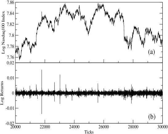
Figure 1: Sample of the tick-by-tick time series of the Nasdaq100(a), as well as the corresponding returns (b).

2 Wavelet Method

With the recent development of the interdisciplinary area of complexity, many physicists have started to study the dynamical properties of stock markets [13, 14]. Empirical results have shown that the time series of financial returns show a behaviour similar to hydrodynamic turbulence [15, 16] – although differences have also been pointed out [16]. Both the spatial velocity fluctuations in turbulent flows and the stock market returns show an intermittent behaviour, characterized by broad tails in the probability distribution function (PDF), and a non-linear multifractal spectrum [15]. The PDF for the normalized logarithmic returns,

$$r(t)=\frac{R(t)-\langle R(t)\rangle_{l}}{\sigma(R(t))},$$ (1)

where $\langle\ldots\rangle_{l}$ is the average over the length of the sample, $l$, and $\sigma$ the standard deviation, is plotted in Fig. 2. The departure from a Gaussian behaviour is evident, in particular, in the peak of the distribution and in the broad tails, which are related to extreme events.

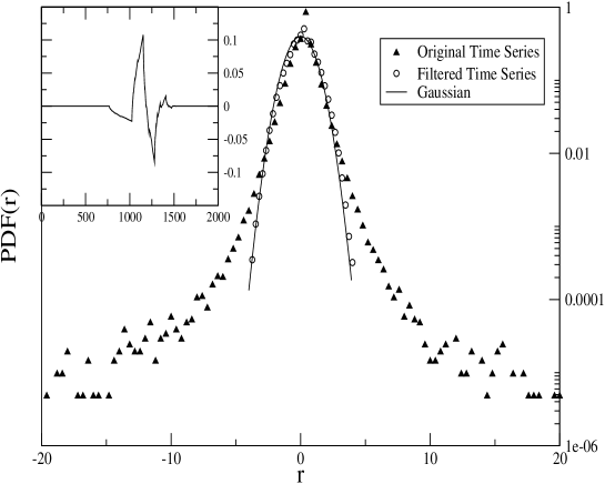
Figure 2: PDF of the logarithmic returns of the Nasdaq100 index before (triangles) and after filtering (circles), with $C=2$. The original time series is reduced to the level of noise. A Gaussian distribution is plotted for comparison. The insert shows the fourth member of the Daubechies wavelets used in the filtering.

The empirical analogies between turbulence and the stock market may suggest the existence of a temporal information cascade for the latter [15]. This is equivalent to assuming that various traders require different information according to their specific strategies. In this way different time scales become involved in the trading process. In the present work we use a wavelet method in order to study multi-scale market dynamics.

The wavelet transform is a relatively new tool for the study of intermittent and multifractal signals [19]. The approach enables one to decompose the signal in terms of scale and time units and so to separate its coherent parts – that is, the bursty periods related to the tails of the PDF – from the noise-like background, thus enabling an independent study of the intermittent and the quiescent intervals [20].

The continuous wavelet transform (CWT) is defined as the scalar product of the analyzed signal, $f(t)$, at scale $\lambda$ and time $t$, with a real or complex “mother wavelet”, $\psi(t)$:

$$W_{T}f(t)=\langle f,\psi_{\lambda,t}\rangle=\int f(u)\bar{\psi}_{\lambda,t}(u)du=\frac{1}{\sqrt{\lambda}}\int f(u)\bar{\psi}(\frac{u-t}{\lambda})du.$$ (2)

The idea behind the wavelet transform is similar to that of windowed Fourier analysis and it can be shown that the scale parameter is indeed inversely proportional to the classic Fourier frequency. The main difference between the two techniques lies in the resolution in the time-frequency domain. In the Fourier analysis the resolution is scale independent, leading to aliasing of high and low frequency components that do not fall into the frequency range of the window. However in the wavelet decomposition the resolution changes according to the scale (i.e. frequency). At smaller scales the temporal resolution increases at the expense of frequency localization, while for large scales we have the opposite. For this reason the wavelet transform is considered a sort of mathematical “microscope”. While the Fourier analysis is still an appropriate method for the study of harmonic signals, where the information is equally distributed, the wavelet approach becomes fundamental when the signal is intermittent and the information localized.

The CWT of Eq.(2) is a powerful tool to graphically identify coherent events, but it contains a lot of redundancy in the coefficients. For a time series analysis it is often preferable to use a discrete wavelet transform (DWT). The DWT can be seen as a appropriate sub-sampling of Eq.(2) using dyadic scales. That is, one chooses $\lambda=2^{j}$, for $j=0,...,L-1$, where $L$ is the number of scales involved, and the temporal coefficients are separated by multiples of $\lambda$ for each dyadic scale, $t=n2^{j}$, with $n$ being the index of the coefficient at the $j$th scale. The DWT coefficients, $W_{j,n}$, can then be expressed as

$$W_{j,n}=\langle f,\psi_{j,n}\rangle=2^{-j/2}\int f(u)\psi(2^{-j}u-n)du,$$ (3)

where $\psi_{j,n}$ is the discretely scaled and shifted version of the mother wavelet. The wavelet coefficients are a measure of the correlation between the original signal, $f(t)$, and the mother wavelet, $\psi(t)$ at scale $j$ and time $n$. In order to be a wavelet, the function $\psi(t)$ must satisfy some conditions. First it has to be well localized in both real and Fourier space and second the following relation

$$C_{\psi}=2\pi\int_{-\infty}^{+\infty}\frac{|\hat{\psi}(k)|^{2}}{k}dk<\infty,$$ (4)

must hold, where $\hat{\psi}(k)$ is the Fourier transform of $\psi(t)$. The requirement expressed by Eq.(4) is called admissibility and it guarantees the existence of the inverse wavelet transform. The previous conditions are generally satisfied if the mother wavelet is an oscillatory function around zero, with a rapidly decaying envelope. Moreover, for the DWT, if the set of the mother wavelet and its translated and scaled copies form an orthonormal basis for all functions having a finite squared modulus, then the energy of the starting signal is conserved in the wavelet coefficients. This property is, of course, extremely important when analyzing physical time series [21]. More comprehensive discussions on the wavelet properties and applications are given in Refs. [22] and [19]. Among the many orthonormal bases known, in our analysis we use the fourth member of the Daubechies wavelets [22], shown in the insert of Fig. 2. The spiky form of this wavelet insures a strong correlation for the bursty events in the time series. The following method of analysis has also been tested with other wavelets and the results are qualitatively unchanged.

The importance of the wavelet transform in the study of turbulent signals lies in the fact that the large amplitude wavelet coefficients are related to the extreme events in the tails of the PDF, while the laminar or quiescent periods are related to the ones with smaller amplitude [21]. In this way it is possible to define a criterion whereby one can filter the time series of the coefficients depending on the specific needs. In our case we adopt the method used in Ref. [21] and originally proposed by Katul et al [23]. In this method wavelet coefficients that exceed a fixed threshold are set to zero, according to

$$\tilde{W}_{j,n}=\left\{\begin{array}[]{ccc}W_{j,n}&{\rm if}&W^{2}_{j,n}<C\cdot\langle W^{2}_{j,n}\rangle_{n},\\ 0&{\rm otherwise},\end{array}\right.$$ (5)

here $\langle\ldots\rangle_{n}$ denotes the average over the time parameters at a certain scale and $C$ is the threshold coefficient. In the next section we will see that the precise value of the parameter $C$ is not critical for our analysis. However it is possible to tune $C$ such that only Gaussian noise is filtered. Once we have filtered the wavelet coefficients $\tilde{W}_{j,n}$ we perform an inverse wavelet transform, obtaining a smoothed version, Fig. 3(b), of the original time series, Fig. 3(a). The residuals of the original time series with the filtered one correspond to the bursty periods which we aim to study, Fig. 3(c).

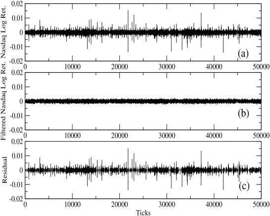
Figure 3: A sample of the original time series of logarithmic returns for the Nasdaq100 is shown in (a), same as Fig. 1(b). The filtered version is shown in (b). The noise-like behaviour of this time series is evident. The residual time series is shown in (c). This corresponds to the high activity periods of the time series, related to the broad wings of the PDF. The cut-off parameter in this case is $C=2$.

3 Data Analysis

In the previous section we have introduced the wavelet method in order to distinguish periods of high activity and periods of low or noise-like activity. The results are shown in Fig. 3 for $C=2$. In order to choose an appropriate cut-off for the wavelet energy, that is to fix a proper $C$, we tune this parameter until the statistics on the kurtosis and the skewness of the filtered time series approach the noise levels, namely 3 and 0 respectively. Once we have isolated the noise part of the time series we are able to perform a reliable statistical analysis on the coherent events of the residual time series, Fig. 3(c). In particular, we define coherent events as the periods of the residual time series in which the volatility, $v(t)\equiv|R(t)|$, is above a small threshold, $\epsilon\approx 0$. The smoothing procedure is emphasized by the change in the PDFs before and after the filtering – as shown in Fig. 2. From this plot it is clear how the broad tails, related to the high energy events that we want to study, and the associated central peak are cut-off by the filtering procedure. The filtered time series is basically a Gaussian, related to a noise process.

A parallel between avalanches in the classical sandpile models (BTW models) exhibiting SOC [1] and the previously defined coherent events in the stock market is straightforward. In order to test the relation between the two, we make use of some properties of the BTW models. In particular, we use the fact that the avalanche size distribution and the avalanche duration are distributed according to power laws, while the laminar, or waiting times between avalanches are exponentially distributed, reflecting the lack of any temporal correlation between them [24, 25]. This is equivalent to stating that the triggering process has no memory.

Similarly to the dissipated energy in a turbulent flow, we define an avalanche, $V$, in the market context as the integrated value of the squared volatility, over each coherent event of the residual time series. The duration, $D_{t}$, is defined as the interval of time between the beginning and the end of a coherent event, while the laminar time, $L_{t}$, is the time elapsing between the end of an event and the beginning of the next one. The time series for $V$, $D_{t}$ and $L_{t}$ are plotted in Fig. 4 for $C=2$.

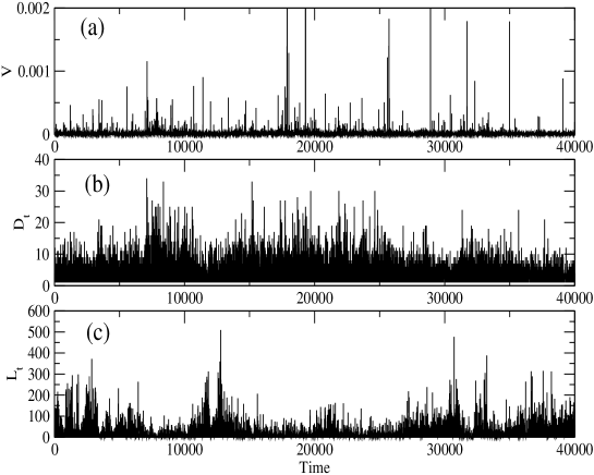
Figure 4: Time series for the avalanche volumes, $V$, for the Nasdaq100, (a); duration, $D_{t}$, of the avalanches, (b); and laminar times, $L_{t}$ (c). The plots are obtained using $C=2$ as the filtering parameter.

The results for the statistical analysis for the Nasdaq100 index are shown in Figs. 5, 6 and 7, respectively, for the avalanche size, duration and laminar times. The robustness of our method has been tested against the energy threshold, we perform the same analysis with different values of $C$.

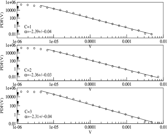
Figure 5: Probability distribution function for the avalanche sizes tested against several values of $C$. The power law behaviour is robust with respect to this parameter.

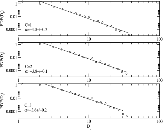
Figure 6: The duration of the high activity periods show a power law distribution, independent of the value of $C$.

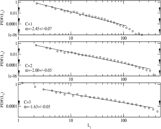
Figure 7: Power law distribution of laminar times for different values of $C$.

A power law relation is clearly evident for all the quantities investigated, largely independent of the specific value of $C$. At this point is important to stress the difference in the distribution of laminar times between the BTW model and the data analyzed. As explained previously, the BTW model shows an exponential distribution for the latter, derived from a Poisson process with no memory [24, 25]. The power law distribution found for the stock market instead implies the existence of temporal correlations between coherent events. This empirical result rules-out the hypothesis that the stock market is in a SOC state, at least in relation to the classical sandpile models.

In order to extend the study of the avalanche behaviour to different markets, we perform the same analysis over the 30 minute returns for the S&P ASX50. The results are shown in Figs. 8, 9 and  10. While the power law scaling for the laminar times is still very clear, the power law for the other quantities is to less precise, perhaps reflecting a different underlying dynamics compared to the Nasdaq100. On the other hand it is also important to stress the difference in length of the two time series analyzed. While for the Nasdaq100 we used $2^{19}$ data points, only $2^{14}$ were available for the S&P ASX50, making the first study statistically more reliable.

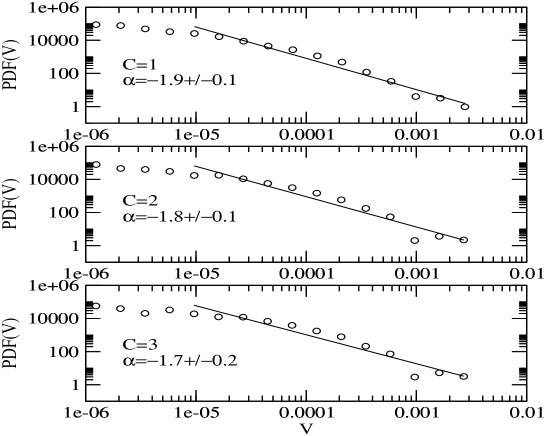
Figure 8: Probability distribution function for the avalanche sizes for the S&P ASX50, from 20/1/1988 to 1/5/2002.

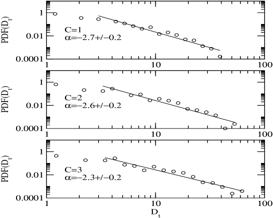
Figure 9: Distribution of the duration of the coherent events for the S&P ASX50.

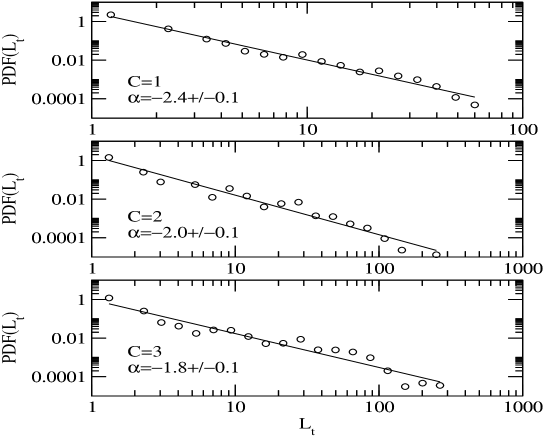
Figure 10: Distribution of laminar times for S&P ASX50 index.

We also investigate the possibility of differences between high frequency data and daily closures by considering a sample of $2^{14}$ daily closures of the Dow Jones index, from 2/2/1939 to 13/4/2004. The power law behaviour is consistent with that found for the high frequency data, as shown in Figs. 11,  12 and  13.

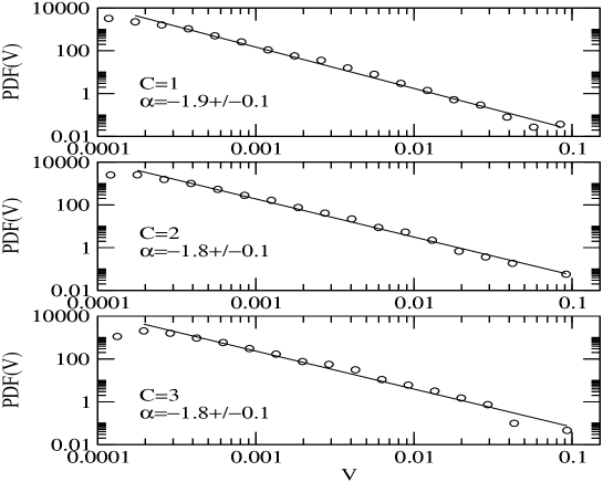
Figure 11: Probability distribution function for the avalanche sizes for the Dow Jones daily closures, from 2/2/1939 to 13/4/2004.

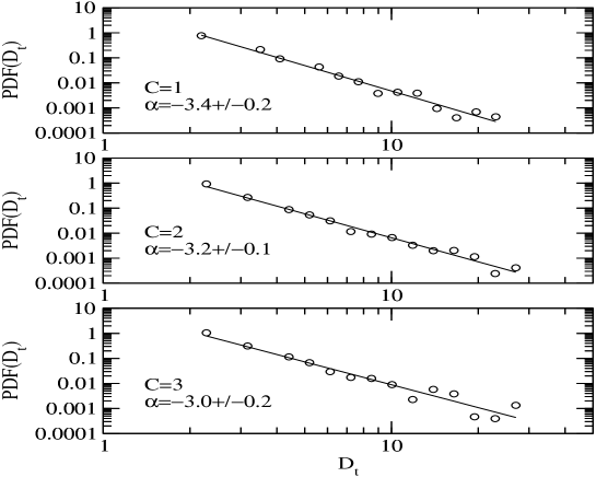
Figure 12: Distribution of the duration of the Dow Jones index.

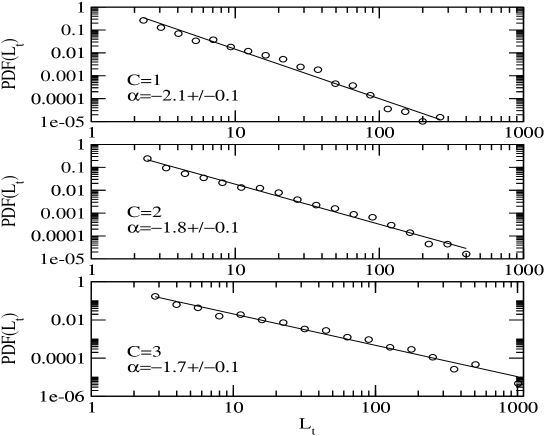
Figure 13: Distribution of laminar times for the Dow Jones index.

4 Discussion

Similar power law behaviour for $V$, $D_{t}$ and $L_{t}$ has been found in the context of solar flaring [24] and in geophysical time-series [21]. In the case of solar flaring, Boffetta et. al [24] have shown that the characteristic distributions found empirically are more similar to the dissipative behaviour of the shell model for turbulence [26, 27] than to SOC. On the other hand the intermittency in turbulent flows discussed in Sec 2 is believed to be the result of a non-linear energy cascade that generates non-Gaussian events at small scales [17] where the shape of the PDF is extremely leptokurtic. At larger scales the spatial correlation decreases and the PDF converges toward a Gaussian. These features imply the absence of global self-similarity – which, as we have noted, is an intrinsic component of SOC models [18].

Freeman et. al [28] have argued that, although an exponential distribution holds for classical sandpile models, there exist some non-conservative modifications of the BTW models in which departures from an exponential behaviour for the $L_{t}$ distribution [29, 30, 31, 32] are observed in the presence of scale-free dynamics for other relevant parameters. The question remains whether or not these systems are still in a SOC state [28]. If we assume that the power law scaling of the laminar times corresponds to a breakdown of self-organized criticality, then we face the problem of how to explain the observed scale-free behaviour of the non-conservative models. This ambiguity can be resolved if we assume that the system is in a near-SOC state, that is the scaling properties of the system are kept even if it is not exactly critical and temporal correlations may be present [28, 33]. Another possible scenario is related with the existence of temporal correlations in the driver [34, 35]. In this case the power law behavior of the waiting time distribution would be explained and the realization of a SOC state preserved [34, 35].

5 Conclusions

In the present work we have investigated empirically the possible relations between the theory of self-organized criticality and the stock market. The existence of a SOC state for the market would be of great theoretical importance, as this would impose some constraints on the dynamics of this complex system. A bounded attractor in the state space would be implied. Moreover, we would have a better understanding of business cycles.

From the wavelet analysis on a sample of high frequency data for the Nasdaq100 index, we have found that the behaviour of high activity periods, or avalanches, is characterized by power laws in the size, duration and laminar times. The power laws in the avalanche size and duration are a characteristic feature of a critical underlying dynamics in the system, but this is not enough to claim the self-organized critical state. In fact the power law behavior in the laminar time distribution implies a memory process in the triggering driver that is absent in the classical BTW models, where an exponential behavior is expected. This does not rule out completely the hypothesis of underlying self-organized critical dynamics in the market. Non-conservative systems, as for the case of the stock market, near the SOC state can still show power law dynamics even in presence of temporal correlations of the avalanches [28, 33]. Another possible explanation is that the memory process, possibly chaotic, is intrinsic in the driver. In this case the power law behavior of the waiting time distribution would be explained and the realization of a SOC state preserved [34, 35].

These findings extend beyond the Nasdaq100 index analysis. A similar quantitative behaviour has been observed in the S&P ASX50 high frequency data for the Australian market and the daily closures of the Dow Jones index for the American market. At this point it is important to stress that this does not imply that all the markets must display the same identical characteristics. In the case of a near-SOC dynamics, for example, the power law shape of the distribution can be influenced by the degree of dissipation of the system which may change from market to market, implying a non-universal behaviour.

In conclusion, a definitive relation between SOC theory and the stock market has not been found. Rather, we have shown that a memory process is related with periods of high activity. The memory could result from some kind of dissipation of information, similar to turbulence, or possibly a chaotic driver applied to the self-organized critical system. Of course, a combination of the two processes can also be possible. Our future work will be devoted to the study of new tests for self-organized criticality and the implementation of numerical models [36].

References

- [1] P. Bak et al., Phys. Rev. Lett. 59, 381 (1987); P. Bak et al., Phys. Rev. A 38, 364 (1988).
- [2] H. J. Jensen, Self-Organized Criticality: Emergent Complex Behavior in Physical and Biological Systems, (Cambridge University Press, Cambridge, 1998).
- [3] D. L. Turcotte, Rep. Prog. Phys. 62, 1377 (1999).
- [4] E.T. Lu and R.J. Hamilton, Astrophys.J. 380, L89 (1991); E.T. Lu et al., Astrophys.J. 412, 841 (1993).
- [5] T. Chang et al., Advences in Space Environmental Research, Vol.I, (Kluwer Academic Publisher,AH Dordrecht, The Netherlands, 2003); A. Valdiva et al., Advences in Space Environmental Research, Vol.I, (Kluwer Academic Publisher,AH Dordrecht, The Netherlands, 2003).
- [6] P. Bak and C. Tang, J. Geophys. Res. 94, 15 635 (1989); Sornette A. and Sornette D., Europhys. Lett. 9, 197 (1989); Sornette D. et al.,J. Geophys. Res. 95, 17 353 (1990); J. Huang et al., Europhys. Lett. 41, 43 (1998).
- [7] P. Bak and K. Snappen, Phys. Rev. Lett. 71, 4083 (1993).
- [8] K. Nagel and H.J. Herrmann, Physica A 199, 254 (1993); K. Nagel and M. Paczuski, Phys. Rev. E 51, 2909 (1995); T. Nagatani, J.Phys. A:Math.Gen. 28, L119 (1995); T. Nagatani, Fractals 4, 279 (1996).
- [9] D.C. Roberts and D.L. Turcotte, Fractals 6, 351 (1998).
- [10] P. Bak et al.,Ric. Econ. 47, 3 (1993).
- [11] P. Bak et al.,Physica A 246, 430 (1997).
- [12] J. Feigenbaum, Rep. Prog. Phys. 66, 1611 (2003).
- [13] R. N. Mantegna and H. E. Stanley, An Introduction to Econophysics: Correlation and Complexity in Finance, (Cambridge University Press, Cambridge, 1999); J.-P. Bouchard and M. Potters, Theory of Financial Risk, (Cambridge University Press, Cambridge, 1999).
- [14] W. Paul and J. Baschnagel, Stochastic Processes: From Physics to Finance, (Spriger-Verlag, Berlin,1999).
- [15] S. Ghashghaie et al., Nature 381, 767 (1996).
- [16] R. N. Mantegna and H. E. Stanley, Physica A 239, 225 (1997).
- [17] U. Frisch, Turbulence, (Cambridge University Press, Cambridge, 1995).
- [18] V. Carbone et al., Europhys. Lett.,58 (3), 349 (2002).
- [19] M. Farge, Annu. Rev. Fluid Mech. 24, 395 (1992).
- [20] M. Farge et al., Phys. Fluids 11, 2187 (1999).
- [21] P. Kovcs et al. Planet. Space Sci. 49, 1219 (2001).
- [22] I. Daubechies, Comm. Pure Appl. Math. 41 (7), 909 (1988).
- [23] G.G. Katul et al., Wavelets in Geophysics, pp. 81-105, (Academic, San Diego, Calif. 1994)
- [24] G. Boffetta et al., Phys. Rev. Lett. 83, 4662 (1999).
- [25] M.S. Wheatland et al., Astrophys.J.509, 448 (1998).
- [26] T. Bohr et. al., Dynamical System Approach to Turbulence, (Cambridge University Press, Cambridge, 1998).
- [27] P. Giuliani and V. Carbone, Europhys. Lett. 43, 527 (1998).
- [28] M.P. Freeman et. al., Phys. Rev. E 62, 8794 (2000).
- [29] K. Christensen and Z. Olami, Geophys. Res. Lett. 97, 8729 (1992).
- [30] Z. Olami and K. Christensen, Phys. Rev. A. 46, R1720 (1992).
- [31] T. Hwa and M. Kardar, Phys. Rev. A, 45, 7002 (1992).
- [32] H.F. Chau and K.S. Cheng, Phys. Rev. A, 46, R2981 (1992).
- [33] J.X. Carvalho and C.P.C. Prado, Phys. Rev. Lett., 84, 4006 (2000).
- [34] P. De Los Rios et. al., Phys. Rev. E 56, 4876 (1997).
- [35] R. Sanchez et. al., Phys. Rev. Lett. 88, 068302-1 (2002).
- [36] M. Bartolozzi and A.W. Thomas, Phys. Rev. E 69, 046112 (2004).