Phase diagram for ultracold bosons in optical lattices and superlattices

Abstract

We present an analytic description of the finite-temperature phase diagram of the Bose-Hubbard model, successfully describing the physics of cold bosonic atoms trapped in optical lattices and superlattices. Based on a standard statistical mechanics approach, we provide the exact expression for the boundary between the superfluid and the normal fluid by solving the self-consistency equations involved in the mean-field approximation to the Bose-Hubbard model. The zero-temperature limit of such result supplies an analytic expression for the Mott lobes of superlattices, characterized by a critical fractional filling.

I Introduction

The standing wave produced by the interference among counterpropagating laser beams gives rise to a periodic potential commonly used to fragment and trap clouds of ultracold (possibly condensed) alkali atoms A:BAnderson ; A:Orzel ; A:Morsch . The local minima of such trapping potential are the sites of the so-called optical lattice A:Jaksch . The use of multiple wavelength laser beams allows to obtain superlattices, namely more structured periodic potentials characterized by a spatial modulation of the depth of the lattice wells A:Guidoni97 ; A:Roth03 ; A:Blakie ; CM:Santos ; A:Aizenman .

In the case of bosonic atoms cooled to within the lowest Bloch band of the periodic potential, it can be shown A:Jaksch that the physics of the system is described by the well-known Bose-Hubbard Hamiltonian A:Fisher

$$H\!=\!\sum_{j}\left[\frac{U}{2}n_{j}(n_{j}\!-\!1)\!-\!(\mu-v_{j})n_{j}\!-\!ta_{j}\sum_{h\sim j}\tau_{jh}a_{h}^{+}\right]$$ (1)

where the subscripts $j,h$ label the sites of the optical lattice, $a_{j}^{+}$ ($a_{j}$) creates (annihilates) a boson at site $j$, $n_{j}=a_{j}^{+}a_{j}$ counts the bosons at site $j$, and the symbol $\sim$ restricts the sum over $h$ to the nearest neighbours of $j$. This is obtained by a scheme analogous to the tight-binding approximation commonly adopted for the study of electrons in solids, i.e. by expanding the state of the system onto a set of wavefunctions localized at the local minima of the trapping potential. The parameters $U$, $t$, $\tau_{jh}$ and $v_{j}$ are hence given in terms of overlap integrals between the localized wavefunctions at neighbouring sites and the trapping potential. Specifically, $U$ represents the repulsive boson-boson interaction, $v_{j}$ is the local potential at site $j$ and $t\cdot\tau_{jh}$ is the hopping amplitude between sites $j$ and $h$. More in detail, $t$ is a global scaling factor determined by the laser intensity, while $\tau_{jh}=\tau_{hj}$ is a local parameter depending on the details of the optical potential in the region between lattice sites $j$ and $h$ (see Fig. 3 for a schematic representation of the optical superlattices considered in the following). A fine tuning of parameters $v_{j}$, $t$ and $\tau_{ij}$ can be in principle obtained via suitable variations of experimental parameters such as the intensity, the frequency and the geometric setup of the laser beams producing the optical (super)lattice N:Feshback . For generic superlattices $\tau_{jh}$ and $v_{j}$ are periodic functions of the lattice labels , whereas in the case of the usual single-wavelength optical lattices they are usually assumed to be site-independent, so that one can set $\tau_{jh}=1$ and $v_{j}=0$ without loss of generality.

The parameter $\mu$ appearing in Hamiltonian (1) is the usual chemical potential of the grand canonical statistical approach, and is fixed by the total number of bosons in the system.

Hamiltonian (1) is also strictly related to systems other than the one under concern, such as Josephson junction arrays and quantum spin systems on lattices A:FazioPR ; CM:Garcia . The hallmark of such class of systems is no doubt the quantum phase transition between a superfluid and a (Mott) insulator phase A:Fisher originating from the competition between the repulsive and kinetic term of the Hamiltonian, whose magnitude are proportional to the parameters $U$ and $t$, respectively. The fine tuning of these parameters made possible by the striking progress in optical lattice techniques allowed Greiner and co-workers to observe the superfluid-insulator transition in a recent breakthrough experiment A:Greiner . More in general, ultracold neutral atoms make an ideal benchmark for testing the properties of widespread models of condensed matter physics A:Zwerger .

It is worth recalling that the above quantum phase transition is rigorously present only at zero temperature B:Sachdev , whereas at finite temperature thermal fluctuations induce a classical phase transition between a superfluid and a normal phase. However, at sufficiently low temperatures, a remnant of the insulating phase still persists within the normal phase. Indeed in these conditions it is possible to observe a sharp crossover between a compressible normal fluid and a phase characterized by a vanishing compressibility, which, for all practical purposes, can be considered a Mott insulator A:Sheshadri ; A:Dicker .

The zero-temperature phase diagram of the Bose-Hubbard model has been widely studied using a variety of techniques, including the mean-field approaches A:Sheshadri ; A:Amico ; A:vanOosten ; CM:Jain , strong coupling perturbative expansion A:Freericks1 ; A:Elstner99a ; CM:scpe , density matrix renormalization group A:Kuehner and of course Quantum Monte Carlo simulations A:Batrouni ; A:Kashurnikov96 .

As to the finite-temperature case, some early numerical results concerning the homogeneous lattice are reported in Ref. A:Kampf, , where a coarse graining mean-field approach is adopted, and in Ref. A:Sheshadri, , based on a random phase approximation refining the mean-field approach therein proposed. In Ref. A:Amico96, the weak-repulsion limit is addressed, and some results are obtained numerically within a different mean-field scheme, based on the linearization of the repulsive term rather than on the decoupling of the hopping term, like in Ref. A:Sheshadri, . Quite recently, Dickerscheid and co-workers A:Dicker adopted a slave-boson technique allowing to include the finite temperature effects in the mean-field picture of Ref. A:Sheshadri, . The ongoing interest in the issue under examination is further confirmed by Ref. CM:Giampaolo, —where a multiband model is addressed — and Ref. CM:Plimak, — where some analytic results are obtained by interpolating two different perturbative schemes and subsequently checked against density matrix renormalization group simulations. All of the above listed results have been obtained either numerically or applying some further approximation such as introducing tight restrictions on the number of particles per site. Note however that, despite such restrictions, the latter approach may prove sufficient to give satisfactory results within circumscribed regions of the phase diagram.

Here we focus on the mean-field approach to Hamiltonian (1) proposed by Sheshadri et al. A:Sheshadri , and, for any temperature $T$, we determine analytically the boundary of the superfluid domain of the phase diagram thereof. In this framework the phases of the system are characterized in terms of the so-called superfluid order parameter, to be determined as the stable fixed point of a self-consistency equation. Detailedly, this parameter vanishes in the normal fluid phase, whereas it has a finite value in the superfluid phase. We determine the critical boundary between these phases by discussing the (parameter dependent) stability of the fixed point corresponding to the normal phase. Furthermore we discuss the above-mentioned crossover between the compressible normal fluid and the insulator-like phase taking place outside the superfluid domain. Other than the usual $d$-dimensional homogeneous lattice, we consider a generic one-dimensional $\ell$-periodic superlattice, providing a solution in terms of the maximal eigenvalue of a $\ell\times\ell$-matrix. Explicit results are given for the the 2-periodic and for a special case of the 3-periodic superlattice, where such maximal eigenvalue can be easily worked out. The zero-temperature phase-diagram of the above mentioned systems is recovered taking the appropriate limit in our results. In particular, for superlattices, we find that rational filling lobes appear besides the usual integer-filling Mott domains. Also, we observe that the occurrence of the latter can be prevented with suitable choices of the supercell potential profile. All of our results prove equivalent to those obtained adopting the standard numerical algorithm, based on a self-consistent iterative procedure.

The plan of this paper is as follows. In section II we briefly recall the mean-field approach presented in Ref. A:Sheshadri, and introduce the finite-temperature self-consistency condition. In Section III we shortly address the homogeneous lattice case, providing the exact expression for the boundary of the superfluid domain, and discussing the crossover between the compressible normal fluid and a insulator-like phase. These results are extended to the case of periodic superlattices in Sec. IV, where the two above-mentioned special cases are explicitly considered. Most of the technical details of our derivation are confined to Appendix A. Section V contains our conclusions.

II Mean Field Approximation

The mean-field approach to the Bose-Hubbard model introduced by Sheshadri and co-workers A:Sheshadri relies on the standard approximation

$$a_{j}a_{h}^{+}\approx\langle a_{j}\rangle a_{h}^{+}+a_{j}\langle a_{h}^{+}\rangle-\langle a_{j}\rangle\langle a_{h}^{+}\rangle$$ (2)

where $\alpha_{j}\equiv\langle a_{j}\rangle=\langle a_{j}^{+}\rangle$ is the so-called superfluid parameter N:real , to be determined self-consistently. Indeed, equation (2) allows to recast Hamiltonian (1) as the sum of terms containing on-site operators only:

$${\cal H} = \sum_{j=1}^{M}{\cal H}_{j}$$ (3)

$${\cal H}_{j} = \frac{U}{2}n_{j}(n_{j}-1)-(\mu-v_{j})n_{j}$$ (4)

$$-t\left(a_{j}+a_{j}^{+}-\alpha_{j}\right)\sum_{h\sim j}\tau_{jh}\alpha_{h}$$

where $M$ is the number of lattice sites. Note that, unlike Hamiltonian (1), the mean-field Hamiltonian $\cal H$ features single boson terms, and therefore it does not conserve the total number of bosons.

A qualitative zero-temperature phase diagram of the BH model can be obtained by evaluating the expectation value $\langle\cdot\rangle$ on the ground state of Hamiltonian (3). Such evaluation must be performed self-consistently, since the ground state of $\cal H$ itself depends on the set of superfluid parameters $\{\alpha_{j}\}$. In the particular case of homogeneous lattices, translational invariance yields $\alpha_{j}=\alpha$, and one is left with ($M$ identical copies of) a single-site problem. The resulting phase diagram consists of a superfluid region, where $\alpha~{}>~{}0$, and a series of Mott-insulator lobes, where $\alpha=0$ and the local density $\langle n_{j}\rangle$ is pinned to an integer value (and hence the system is in an incompressible state, $\partial_{\mu}\langle n_{j}\rangle=0$ ). The boundaries of these Mott lobes have been determined numerically in the original paper A:Sheshadri , while their analytical expression has been reported in a quite recent work A:vanOosten .

More in general this mean-field approach has been adopted for studying the superfluid-insulator transition in some inhomogeneous situations. An harmonic confining potential $v_{j}\propto(j-j_{0})^{2}$ is considered in Ref. A:Polkov, , whereas the effect of topological inhomogeneity is addressed in Ref. A:BHComb, .

Here we are interested in the thermodynamics of the system, and we adopt the standard grand-canonical statistical mechanic approach,

$$\langle{\cal O}\rangle=\frac{{\rm Tr}({\cal O}e^{-\beta{\cal H}})}{{\rm Tr}(e^{-\beta{\cal H}})},$$ (5)

where the trace is evaluated on the whole Fock space. Exploiting the site-decoupling of the mean-field Hamiltonian ${\cal H}$, Eq. (3), the self-consistency conditions become

$$\alpha_{j}\!\! = \!\!\langle a_{j}\rangle=\frac{{\rm Tr}(a_{j}e^{-\beta{\cal H}})}{{\rm Tr}(e^{-\beta{\cal H}})}$$ (6)

$$= \!\!\frac{{\rm Tr}(a_{j}e^{-\beta{\cal H}_{j}})\prod_{k\neq j}{\rm Tr}(e^{-\beta{\cal H}_{k}})}{\prod_{k=1}^{M}{\rm Tr}(e^{-\beta{\cal H}_{k}})}\!=\!\frac{{\rm Tr}(a_{j}e^{-\beta{\cal H}_{j}})}{{\rm Tr}(e^{-\beta{\cal H}_{j}})}$$

where the traces in the second line are evaluated on the single site Fock space. Note that the superfluid parameters $\alpha_{j}$ can be safely assumed to be real since both ${\cal H}_{j}$ and $a_{j}$ are real operators.

In the following sections we illustrate how it is possible to determine analytically the critical condition for superfluidity, i.e. for the existence of a stable solution of the self-consistency equations (6) with $\alpha_{j}\neq 0$.

III Homogeneous case

When $v_{j}=0$ and $\tau_{jk}=\tau$ the system is translationally invariant and, similar to the above-recalled zero-temperature case, Eqs. (6) reduce to ($M$ identical copies of) a single consistency equation. Dropping the site-labeling subscripts one gets $\alpha_{j}=\alpha=\langle a\rangle$ and

$${\cal H}_{j}=\bar{\cal H}=\frac{U}{2}n(n-1)-\mu n-2d\,t\alpha(a+a^{+})$$ (7)

where $d$ is the dimension of the lattice and we discarded the constant term $2td\alpha^{2}$ since it can be factored out from both the numerator and the denominator of Eq. (5).

In this simple case the self-consistency constraint, Eq. (6), depends on the (site-independent) superfluid parameter $\alpha$, and it is met when the latter is a stable fixed point. It is easy to check that $\alpha=0$ is a fixed point of Eq. (6) whose stability depends on the parameters $U$, $\mu$ and $t$. In particular, when $\alpha=0$ is unstable, a stable solution $\alpha>0$ is expected and the system is in a superfluid state.

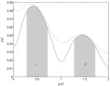
Figure 1: Finite temperature mean-field phase diagram for the homogeneous one-dimensional lattice. The dotted, solid and dashed lines are the critical curves, Eq. (8), for $T/U=0$, $T/U=0.04$ and $T/U=0.1$, respectively. In every case, the superfluid domain is above the relevant critical curve. For $T/U=0$, the region below the (dotted) critical curve consists of two disjoint Mott lobes. For $T/U=0.04$ (solid curve) a sharp crossover between a normal fluid phase and a insulator-like phase is present. The gray areas are the insulator-like regions as evaluated setting $\epsilon=10^{-3}$ in Eq. (12). As discussed in the text, the particle density is very close to an integer value (also shown) inside these regions. For $T/U=0.1$ (dashed curve) no insulator-like regions are present (for the same value of $\epsilon$).

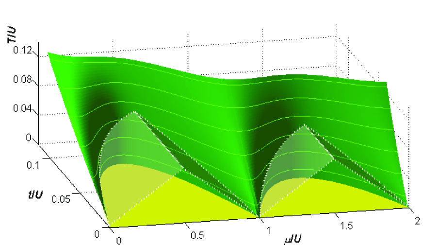
Figure 2: (Color online) Three dimensional representation of the finite-temperature mean-field phase diagram for a homogeneous one-dimensional lattice. Dark gray (green): critical surface, Eq. (8). Light gray (yellow): zero-temperature Mott lobes. White-rimmed transparent surfaces: boundaries between the insulator-like (below) and normal fluid (above) regions. Figure 1 is obtained by cross-sectioning this figure at the relevant values of $T/U$.

In Appendix A we show that the critical curve defining the superfluid domain border is

$$t_{c}(U,\mu,\beta)=\frac{\sum_{k=0}^{\infty}e^{\beta(\mu k-\frac{U}{2}k(k-1))}}{2d\sum_{k=0}^{\infty}Q_{k}(U,\mu)e^{\beta(\mu k-\frac{U}{2}k(k-1))}}$$ (8)

where

$$Q_{k}(U,\mu)=\frac{\mu+U}{(\mu-Uk)[U(k-1)-\mu]}$$ (9)

Note that when $\alpha=0$ the expectation value of the particle density does not depend on $t$, being simply

$$\rho(U,\mu,\beta)=\langle n\rangle=\frac{\sum_{k=0}^{\infty}ke^{\beta(\mu k-\frac{U}{2}k(k-1))}}{\sum_{k=0}^{\infty}e^{\beta(\mu k-\frac{U}{2}k(k-1))}}$$ (10)

Hence, unlike the zero-temperature case, the $\alpha=0$ region in general does not yield integer particle density. However it can be shown that, for sufficiently low temperatures, there are $\mu$ intervals where $\rho(U,\mu,\beta)$ is practically constant. This happens when a single term of the sums in (10), whose label we denote $k^{*}$, outweighs the remaining terms, i.e. when

$$e^{-\frac{\beta U}{2}(k^{*}-\frac{\mu}{U}-\frac{1}{2})^{2}}>\epsilon^{-1}e^{-\frac{\beta U}{2}(k^{*}\pm 1-\frac{\mu}{U}-\frac{1}{2})^{2}}$$ (11)

where $\epsilon$ is a small parameter. The last equation identifies the interval

$$k^{*}-1-\frac{\ln(\epsilon)}{\beta U}<\frac{\mu}{U}<k^{*}+\frac{\ln(\epsilon)}{\beta U}$$ (12)

where $\rho(U,\mu,\beta)\approx k^{*}$. More precisely, expanding Eq. (10) with respect to $\epsilon$ and considering only the linear order, one gets $|\rho-k^{*}|\approx\epsilon$. In the normal fluid region between two subsequent intervals of the form (12) the particle density can be described considering only the terms $k^{*}$ and $k^{*}+1$ in Eq. (10)

$$\rho(U,\mu,\beta)\approx\frac{k^{*}+(k^{*}+1)e^{\beta(\mu-Uk^{*})}}{1+e^{\beta(\mu-Uk^{*})}}$$

Last equation clearly shows the crossover between two subsequent insulator-like regions. Of course, when $\beta<-2\ln(\epsilon)/U$ there is no $\mu$ satisfying the Eq. (12), and the plateau-like behaviour of $\rho(U,\mu,\beta)$ disappears.

The same line of reasoning allows to obtain quite straightforwardly the exact phase diagram of the model in the zero temperature limit A:vanOosten . Indeed, when $\beta\to\infty$ only the terms labeled by $k=k^{*}$ survive in Eq. (8), so that the critical curve in the $\mu/U$-$t/U$ phase diagram is

$$\frac{t_{c}(U,\mu,\infty)}{U}=\frac{(\frac{\mu}{U}-k^{*})(k^{*}-1-\frac{\mu}{U})}{2d(\frac{\mu}{U}+1)}$$ (13)

and, according to Eq. (12), $\mu\in[k^{*}-1,k^{*}]$.

The boundary of the superfluid domain at different temperatures, along with the crossover between the normal fluid and the Mott insulator (when present) is shown in Figs. 1 and  2 for a homogeneous lattice with $d=1$. As it is evident from Eq. (8), the results for $d>1$ are obtained by a suitable rescaling of $t_{c}$.

IV Superlattices

We now turn to the case of superlattices, where the parameters appearing in Hamiltonian (3) are periodic functions of the site label. Our approach can be applied to a generic $d$-dimensional superlattice, but, for the sake of clarity, here we focus on the one-dimensional $\ell$-periodic case, $v_{j}=v_{j+\ell}$ and $\tau_{j,h}=(\delta_{h,j+1}+\delta_{h,j-1})\tau_{j+\ell,h+\ell}$. Note that this choice is not merely dictated by the ensuing notational simplification, but also experimentally relevant A:Morsch ; A:Orzel .

Since the superfluid parameters mirror the $\ell$-periodicity of the superlattice, $\alpha_{j}=\alpha_{j+\ell}$, the self-consistency conditions (6) reduce to $\ell$ independent equations. As in the homogeneous case, the choice $\alpha_{h}=0$ for all $h$’s is a fixed point of Eq. (6), and only when it is unstable the system is expected to be in a superfluid state. According to a standard approach, the stability of such fixed point can be discussed based on the spectrum of the matrix linearizing the map defined by Eq. (6) in the vicinity of the configuration $\alpha_{h}=0$. More in detail, the fixed point is stable only if the modulus of the maximal eigenvalue of such matrix is lower than one. By adopting a calculation technique similar to the one of the homogeneous case (see Appendix A), the linearized map turns out to be

$$\alpha_{h}\approx t\sum_{h^{\prime}=1}^{\ell}F_{h,h^{\prime}}\alpha_{h^{\prime}}$$ (14)

where, introducing $\mu_{h}=\mu-v_{h}$ and ${\cal T}_{h,h^{\prime}}=\tau_{h\,h^{\prime}}(\delta_{h\,h^{\prime}+1}+\delta_{h\,h^{\prime}-1})+\tau_{\ell,\ell+1}(\delta_{h\,1}\delta_{h^{\prime}\,\ell}+\delta_{h^{\prime}\,1}\delta_{h\,\ell})$,

$$F_{h,h^{\prime}}={\cal T}_{h,h^{\prime}}\frac{\sum_{k}Q_{k}(U,\mu_{h})\,e^{\beta(\mu_{h}k-\frac{U}{2}k(k-1))}}{\sum_{k}e^{\beta(\mu_{h}k-\frac{U}{2}k(k-1))}},$$ (15)

The function $Q_{k}(U,\mu)$ appearing in Eq. (15) is exactly the same as defined in Eq. (9). Since $F_{h,h^{\prime}}$ is a real and positive matrix, Perron-Frobenius theorem B:Meyer ensures that its maximal eigenvalue $\phi_{\rm M}(\beta,U,\mu)$ is real and positive. Hence, the fixed point $\alpha_{h}=0$ is unstable — and the system behaves like a superfluid — only when $t>t_{c}(\beta,U,\mu)=\phi_{\rm M}^{-1}$. Note that the critical curve separating the superfluid and the normal domains can also be defined as the lowest positive $t_{c}$ such that $P_{F}(t_{c}^{-1})=0$, where $P_{F}(\lambda)$ is the characteristic polynomial of matrix $F_{h,h^{\prime}}$.

In the normal phase ($t<t_{c}$ and $\alpha_{h}=0$, $\forall~{}h$) the local density of particles at site $h$ is:

$$\rho_{h}(U,\mu,\beta)=\langle n_{h}\rangle=\frac{\sum_{k}ke^{\beta((\mu_{h}k-\frac{U}{2}k(k-1))}}{\sum_{k}e^{\beta(\mu_{h}k-\frac{U}{2}k(k-1))}}$$ (16)

Analogously to the homogeneous case, for sufficiently low temperatures there exist intervals of $\mu$ where the local particle density is arbitrarily close to an integer value. In detail, introducing a small parameter $\epsilon$, $|\rho_{h}(U,\mu,\beta)-k^{*}|<\epsilon$ if $\mu\in{\cal M}_{h}(k^{*},\epsilon)$, where

$${\cal M}_{h}(0,\epsilon)=\left]-\infty,v_{h}+\frac{\ln(\epsilon)}{\beta}\right[$$

and, for any positive integer $k^{*}$,

$${\cal M}_{h}(k^{*},\epsilon)\!=\!\left]U(k^{*}\!-\!1)\!+\!v_{h}\!-\!\frac{\ln(\epsilon)}{\beta},Uk^{*}\!+\!v_{h}\!+\!\frac{\ln(\epsilon)}{\beta}\right[.$$ (17)

This in particular means that the average filling

$$\overline{\rho(U,\mu,\beta)}=\ell^{-1}\sum_{h=1}^{\ell}\rho_{h}(U,\mu,\beta)$$ (18)

remains very close to the rational value

$$\overline{k^{*}}=\ell^{-1}\sum_{h=1}^{\ell}k^{*}_{h}$$ (19)

as long as the chemical potential belongs to the interval

$${\cal M}(\{k^{*}_{h}\},\{v_{h}\},\epsilon)=\bigcap_{h=1}^{\ell}{\cal M}_{h}(k_{h}^{*},\epsilon)$$ (20)

where $\{k^{*}_{h}\}_{h=1}^{\ell}$ is a set of non-negative integers such that ${\cal M}\neq\emptyset$. If, conversely, $\alpha_{h}=0$ but $\mu\not\in{\cal M}$, the average filling is not close to a rational number and it significantly varies with varying $\mu$. That is to say, the compressibility is significantly different from zero, and the system behaves like a normal fluid, owing to thermal fluctuations.

In the zero-temperature limit the normal phase behaviour disappears and a (Mott)insulator-superfluid transition is recovered. Similar to the homogeneous case, the $\mu/U$-$t/U$ zero-temperature phase diagram consists of a superfluid domain and a series of insulating Mott-lobes. However, the average filling and compressibility within these lobes are exactly $\overline{k^{*}}$ and zero, respectively. Therefore, as it is expected CM:Santos , we obtain that superlattices can display an insulating-Mott behaviour even for some critical rational fillings.

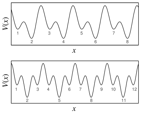
Figure 3: Schematic representation of the $\ell$-periodic optical superlattices explicitly considered in Sec. IV. The lattice sites correspond to the local minima of the optical potential $V(x)$ . Upper panel: $\ell=2$, $v_{j}=v_{j+2}\neq v_{j+1}$, $\tau_{j,j+1}=\tau_{j+2,j+3}\neq\tau_{j+1,j+2}$. Lower panel: $\ell=3$, $v_{j}=v_{j+2}\neq v_{j+1}$, $\tau_{j,j+1}=\tau_{j+1,j+2}\neq\tau_{j+2,j+3}$, $j=3k+1$, $k\in\mathbb{N}$.

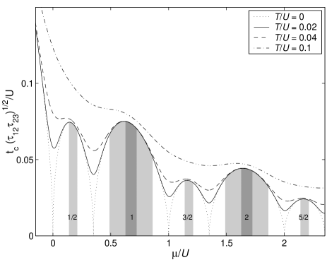
Figure 4: Phase diagram for the superlattice of periodicity $\ell=2$ with parameters $v_{2k}/U=0.35$, $v_{2k+1}/U=0$. Note that the possibly different values of parameters $\tau_{h,h^{\prime}}$ are conveniently absorbed into $t_{c}$ by a multiplicative rescaling. The filled areas correspond to the insulator-like phase for $T=0.02$ (light gray) and $T=0.04$ (dark gray) as evaluated setting $\epsilon=10^{-3}$ in Eq. (20). The rational numbers denote the particle density within the Mott-like domains.

Let us now analyze explicitly the two simple superlattices generated by the trapping potential schematically represented in Fig. 3. The upper panel of this figure corresponds to the simplest choice, namely a superlattice of periodicity $\ell=2$. In this case the maximal eigenvalue of matrix $F$ can be evaluated analytically, and the resulting critical value of $t$ turns out to be

$$t_{c}(U,\mu,\beta)=\sqrt{\frac{1}{F_{1,2}F_{2,1}}}$$ (21)

The ensuing mean-field phase-diagram for a particular choice of the parameters is displayed in Fig. 4. As mentioned above, rational (actually half-integer) filling Mott lobes appear in the zero-temperature phase diagram (dotted curves). As the temperature increases, the regions where the system is in a quasi insulating state shrink and eventually disappear, according to Eq. (20). It is interesting to observe that these regions may disappear at different temperatures, depending on their filling. This is clearly shown in Fig. 4, where the insulating regions relevant to $T=0.02$ (light gray) and $T=0.04$ (dark gray) are shown. Note that in the latter case there are only integer-filling (quasi) insulating regions.

Matrix $F$ can be analytically diagonalized with a limited effort also for the special case of 3-periodic lattice illustrated in the lower panel of Fig. 3, where $v_{1}=v_{3}$ and $\tau_{1,2}=\tau_{2,3}$, so that $F_{1,2}=F_{3,2}$, $F_{1,3}=F_{3,1}$ and $F_{2,1}=F_{2,3}$. After a straightforward calculation one gets

$$t_{c}(U,\mu,\beta)=\frac{2}{F_{1,3}+\sqrt{F_{1,3}^{2}+8F_{1,2}F_{2,1}}}$$ (22)

The relevant phase diagram is shown in Fig. 5.

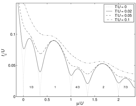
Figure 5: Phase diagram for the superlattice of periodicity $\ell=3$ with parameters $v_{3k}/U=v_{3k+1}/U=0.35$, $v_{3k+2}/U=0$, $\tau_{3k,3k+1}=1/2$ and $\tau_{3k+1,3k+2}=\tau_{3k+2,3k+3}=1$. The rational numbers denote the particle density within the zero-temperature Mott insulator domains.

Note that, similar to the previous example, the zero-temperature Mott lobes can be divided into two classes depending on the relevant particle density, which can be either $k$ or $k+1/3$, where $k\in\mathbb{N}$. This simple behaviour is a consequence of our choice for the local potentials. Of course, more structured choices result into a quite richer phase diagram, where the particle density in the insulator-like regions is an integer multiple of $\ell^{-1}$. Note that some of these multiples are excluded if the energy offset between any two sites $j$ and $h$ within the same supercell is an integer multiple of $U$. Indeed, in this situation, the intervals relevant to sites $j$ and $h$ defined by Eq. (17) overlap exactly. Hence for some set of integers the intersection defined by Eq. (20) is empty. This is exactly what happens in Fig. 5, where $v_{1}-v_{3}=0$. Interestingly, it is possible to devise superlattices where only fractional critical fillings are present, provided that the energy offset between two lattice sites is larger than $U$. This is shown in Fig 6, displaying the zero-temperature phase diagram for a superlattice of periodicity $\ell=4$ as obtained by numerical diagonalization of matrix $F$, Eq. (6).

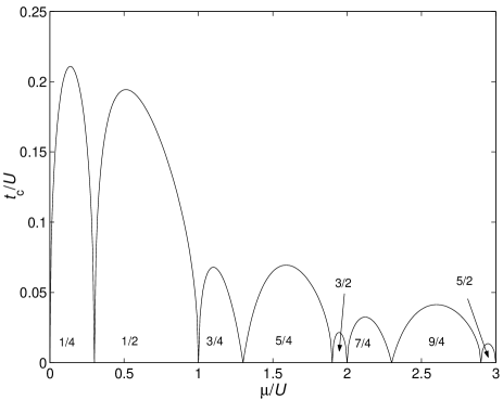
Figure 6: Zero-temperature phase diagram for the superlattice of periodicity $\ell=4$ with parameters $v_{4k}/U=1.9$, $v_{4k+2}/U=0.3$, $v_{4k+1}/U=1.3$, $v_{4k+3}/U=0.0$,$\tau_{k,k+1}=1$. The rational numbers denote the particle density within the Mott insulator domains. Note that, as we discussed in the text, for this particular choice of the well depths there are no integer critical fillings.

V Conclusions

In this paper we extend the mean-field approximation to the Bose-Hubbard model introduced in Ref. A:Sheshadri to include thermal fluctuations. An analytical study of the ensuing self-consistency equations allows us to determine the exact form of the boundary of the superfluid region at any finite temperature. We also quantify the crossover from the normal fluid to the insulator-like phase.

Other than to the homogeneous $d$-dimensional lattice considered in the original reference, we apply our method to a generic one-dimensional $\ell$-periodic superlattice, giving explicit results for $\ell=2$ and a special case of $\ell=3$. Results for more complex one-dimensional superlattices involve the evaluation of the maximal eigenvalue of a $\ell\times\ell$ matrix. Of course, this must be accomplished numerically even for relatively small matrix sizes. Nevertheless this approach much less demanding and more precise than the (equivalent) fully numerical solution of the self-consistency equation. The latter actually involves an iterative self-consistent diagonalization for each point of the the mesh grid describing the phase diagram. Our technique can be extended also to generic $d$-dimensional superlattices, where the size of the matrix to be diagonalized is $s\times s$, $s$ being the number of sites within a supercell. We remark that the boundaries of the superfluid region as evaluated with our method are valid also in the zero-temperature limit, thus providing the phase diagram for the superfluid-insulator quantum transition. In particular this allows to find the analytic expressions of the (mean-field) Mott lobes in the case explicitly considered above.

Appendix A

In this section the analytic expression for the boundary of the superfluid domain is derived in detail for the simple case of the homogeneous lattice. The generalization to the superlattice case is briefly discussed.

As we mention above, in the homogeneous $d$-dimensional case, the self-consistency constraints, Eqs. (6), reduce to a single equation in the variable $\alpha$, i.e. the site-independent superfluid parameter. It proves useful to recast such equation in terms of the quantity $\gamma\equiv\alpha t$ as

$$\gamma=t\frac{{\rm Tr}\left(a\,e^{-\beta\bar{\cal H}}\right)}{Z}=\frac{t}{4d\beta}\frac{d}{d\gamma}\log(Z)\equiv f(\gamma)$$ (23)

where

$$Z={\rm Tr}\left(e^{-\beta\bar{\cal H}}\right)$$ (24)

is the grand-canonical partition function of the single site problem. The additional $1/2$ factor in Eq. (23) ensues from the equality $\alpha=\langle a\rangle=\langle a^{+}\rangle\in{\mathbb{R}}$.

Let us now prove Eq. (8) by discussing the stability character of the fixed point $\gamma=0$ of the map (23). To this aim we truncate the on-site Fock basis considering states up to a given number of particles $n$ and denote $\bar{\cal H}_{n}$ the relevant Hamiltonian matrix. The final result is obtained letting $n$ to infinity.

Introducing the set of eigenvalues of $\bar{\cal H}_{n}$, $\{E_{k}(\gamma)\}_{k=0}^{n}$ , Eq. (23) becomes

$$\gamma=\frac{t}{4d}\frac{\sum_{k=0}^{n}e^{-\beta\,E_{k}(\gamma)}\frac{dE_{k}(\gamma)}{d\gamma}}{\sum_{k=0}^{n}e^{-\beta\,E_{k}(\gamma)}}$$ (25)

Now, since $p_{n}(E_{k}(\gamma);\gamma)=0$, where $p_{n}(\lambda;\gamma)$ is the characteristic polynomial of $\bar{\cal H}_{n}$

$$0 = \frac{dp_{n}(E_{k}(\gamma),\gamma)}{d\gamma}$$ (26)

$$= \Big{[}\frac{dE_{k}(\gamma)}{d\gamma}\partial_{\lambda}p_{n}(\lambda,\gamma)+\partial_{\gamma}p_{n}(\lambda,\gamma)\Big{]}_{\lambda=E_{k}(\gamma)}$$

so that it is possible to write

$$\frac{dE_{k}(\gamma)}{d\gamma}=-\left.\frac{\partial_{\gamma}p_{n}(\lambda,\gamma)}{\partial_{\lambda}p_{n}(\lambda,\gamma)}\right|_{\lambda=E_{k}(\gamma)}$$ (27)

Denoting $p_{n}^{\{k\}}(\lambda;\gamma)$ the characteristic polynomial of the matrix obtained by discarding from $\bar{\cal H}_{n}$ the rows and columns labeled by the set of indices $\{k\}$, and making use of the formula for the derivative of a determinant B:Meyer , one gets

$$\partial_{\lambda}p_{n}(\lambda,\gamma) = \sum_{k=0}^{n}p_{n}^{(k)}(\lambda;\gamma)$$

$$\partial_{\gamma}p_{n}(\lambda,\gamma) = \gamma 8\,d^{2}\left[\sum_{k=1}^{n}k\,p_{n}^{(k,k-1)}(\lambda;\gamma)+P(\gamma)\right]$$

where the polynomial $P(\gamma)$ is homogeneous, so that $P(0)=0$. Hence Eq. (25) becomes

$$\gamma=t\,\gamma\frac{\sum_{k=0}^{n}e^{-\beta\,E_{k}(\gamma)}q_{n}(E_{k};\gamma)}{\sum_{k=0}^{n}e^{-\beta\,E_{k}(\gamma)}}\equiv f(\gamma)$$ (28)

where

$$q_{n}(\lambda;\gamma) = \frac{1}{4d}\frac{\partial_{\gamma}p_{n}(\lambda,\gamma)}{\partial_{\lambda}p_{n}(\lambda,\gamma)}$$ (29)

$$= 2d\frac{\sum_{h=1}^{n}h\,p_{n}^{(h,h-1)}(\lambda;\gamma)+P(\gamma)}{\sum_{h=0}^{n}p_{n}^{(h)}(\lambda;\gamma)}$$

According to standard treatment, $\gamma=0$ is a stable solution of Eq. (28) only if $|\partial_{\gamma}f(\gamma)|_{\gamma=0}<1$, i.e.

$$t<\frac{\sum_{k=0}^{n}e^{-\beta\,E_{k}(0)}}{\sum_{k=0}^{n}q_{n}\left(E_{k}(0);0\right)e^{-\beta\,E_{k}(0)}}$$ (30)

Observing that

$$p_{n}^{\{k\}}(\lambda;0)=\prod_{h\not\in\{k\}}\left(E_{h}(0)-\lambda\right)$$ (31)

one gets

$$q_{n}(E_{k}(0);0)=2d\left[k\,p_{n}^{(k,k-1)}(E_{k}(0);0)+(k+1)\,p_{n}^{(k+1,k)}(E_{k}(0);0)\right]\left[p_{n}^{(k)}(E_{k}(0);0)\right]^{-1}$$ (32)

where we set $p_{n}^{(n,n+1)}(\lambda;\gamma)=p_{n}^{(-1,0)}(\lambda;\gamma)=0$. Now, recalling that $E_{k}(0)=\frac{U}{2}k(k-1)-\mu k$ one gets $\lim_{n\to\infty}q_{n}(E_{k}(0);0)=Q_{k}(U,\mu)$, where the function $Q_{k}$ is defined in Eq. (9). Therefore, the limit $n\to\infty$ of Eq. (30) gives the desired result, Eq. (8).

In the case of superlattices the parameters appearing in Hamiltonian (3) are periodic functions of the site labels. Here we focus on the one-dimensional $\ell$-periodic case, $v_{j}=v_{j+\ell}$ and $\tau_{j,h}=(\delta_{h,j+1}+\delta_{h,j-1})\tau_{j+\ell,h+\ell}$. Since the superfluid parameters mirror the $\ell$-periodicity of the superlattice, $\alpha_{j}=\alpha_{j+\ell}$, the self-consistency conditions (6) reduce to $\ell$ independent equations. Introducing the parameters $\gamma_{h}\equiv t\alpha_{h}$ ($h=1,\dots,\ell$, $\gamma_{\ell+1}\equiv\gamma_{1}$ and $\gamma_{0}\equiv\gamma_{\ell}$), equations (6) can be recast as:

$$\gamma_{h} = \frac{t}{4\beta}\left[\frac{1}{\tau_{h,h-1}}\frac{d\log(Z_{h})}{d\gamma_{h-1}}+\frac{1}{\tau_{h,h+1}}\frac{d\log(Z_{h})}{d\gamma_{h+1}}\right]$$ (33)

$$\equiv f_{h}(\{\gamma_{h^{\prime}}\})$$

where

$$Z_{h}={\rm Tr}\left(e^{-\beta\tilde{\cal H}_{h}}\right)$$ (34)

and

$$\tilde{\cal H}_{h} = \frac{U}{2}n(n-1)-(\mu-v_{h})n-$$ (35)

$$(\tau_{h,h-1}\gamma_{h-1}+\tau_{h,h+1}\gamma_{h+1})(a+a^{+})$$

A procedure similar to that detailedly illustrated in the case of homogeneous lattices allows to linearize Eq. (33), obtaining Eq. (14).

References

- (1) B. Anderson and M. Kasevich, Science 282, 1686 (1998).
- (2) C. Orzel, A. K. Tuchman, M. Fenselau, M. Yasuda and M. A. Kasevich, Science 291, 2386 (2001).
- (3) O. Morsch, J. H. Muller, M. Cristiani, D. Ciampini and E. Arimondo, Phys. Rev. Lett. 87, 140402 (2001).
- (4) D. Jaksch, C. Bruder, J. Cirac, C. Gardiner and P. Zoller, Phys. Rev. Lett. 81, 3108 (1998).
- (5) L. Guidoni, C. Triché, P. Verkerk and G. Grynberg, Phys. Rev. Lett. 79, 3363–3366 (1997).
- (6) R. Roth and K. Burnett, Phys. Rev. A 68, 023604 (2003).
- (7) P. B. Blakie and C. W. Clark, J. Phys. B 37, 1391 (2004).
- (8) L. Santos, M. Baranov, J. Cirac, H.-U. Everts, H. Fehrmann and M. Lewenstein, e-print cond-mat/0401502 (2004).
- (9) M. Aizenman, E. Lieb, R. Seiringer, J. Solovej and J. Yngvason, e-print cond-mat/0403240 (2004).
- (10) M. Fisher, P. Weichman, G. Grinstein and D. S. Fisher, Phys. Rev. B 40, 546 (1989).
- (11) The boson interaction can be also tuned experimentally making use of Feshback resonances.
- (12) R. Fazio and H. van der Zant, Phys. Rep. 355, 235 (2001).
- (13) J. J. García-Ripoll, M. Martin-Delgado and J. I. Cirac, e-print cond-mat/0404566 (2004).
- (14) M. Greiner, I. Bloch, O. Mandel, T. W. Hansch and T. Esslinger, Phys. Rev. Lett. 87, 160405 (2001).
- (15) W. Zwerger, J. Opt. B 5, S9 (2003).
- (16) S. Sachdev, Quantum Phase Transitions, Cambridge University Press, (1999).
- (17) K. Sheshadri, H. Krishnamurthy, R. Pandit and T. Ramakrishnan, Europhys. Lett. 22, 257 (1993).
- (18) D. Dickerscheid, D. van Oosten, P. Denteneer and H. Stoof, Phys. Rev. A 68, 043623 (2003).
- (19) L. Amico and V. Penna, Phys. Rev. Lett. 80, 2189 (1998).
- (20) D. van Oosten, P. van der Straten and H. Stoof, Phys. Rev. A 63, 053601 (2001).
- (21) P. Jain and C. Gardiner, e-print cond-mat/0404642 (2004).
- (22) J. K. Freericks and M. Monien, Europhys. Lett. 26, 545–550 (1994).
- (23) P. Buonsante, V. Penna and A. Vezzani, e-print cond-mat/0406467 (2004).
- (24) N. Elstner and H. Monien, Phys. Rev. B 59, 12184 (1999).
- (25) T. Kühner and H. Monien, Phys. Rev. B 58, R14741 (1998).
- (26) G. Batrouni, R. Scalettar and G. Zimanyi, Phys. Rev. Lett. 65, 1765 (1990).
- (27) V. Kashurnikov, A. Krasavin and B. Svistunov, JETP Lett. 64, 99 (1996).
- (28) A. Kampf and G. Zimanyi, Phys. Rev. B 47, 279 (1993).
- (29) L. Amico, M. Rasetti and R. Zecchina, Physica A 230, 300 (1996).
- (30) S. Giampaolo, F. Illuminati, G. Mazzarella and S. D. Siena, e-print cond-mat/0403145 (2004).
- (31) L. Plimak, M. Fleischhauer and M. Olsen, e-print cond-mat/0309587 (2004).
- (32) The superfluid parameters are real since the operators and have a real representation on the Fock basis.
- (33) A. Polkovnikov, S. Sachdev and S. Girvin, Phys. Rev. A 66, 053607 (2002).
- (34) P. Buonsante, R. Burioni, D. Cassi, V. Penna and A. Vezzani, e-print cond-mat/0405520 (2004).
- (35) C. Meyer, Matrix Analysis and Applied Linear Algebra, SIAM, (2001).