Stochastic equation for a jumping process with long-time correlations
Abstract
A jumping process, defined in terms of jump size distribution and waiting time distribution, is presented. The jumping rate depends on the process value. The process, which is Markovian and stationary, relaxes to an equilibrium and is characterized by the power-law autocorrelation function. Therefore, it can serve as a model of the noise as well as a model of the stochastic force in the generalized Langevin equation. This equation is solved for the noise correlations ; the resulting velocity distribution has sharply falling tails. The system preserves the memory about the initial condition for a very long time.
pacs:
05.40.-a, 02.50.-r, 05.10.GgI Introduction
A jumping process can be defined in terms of two probability distributions which determine a jump size and a waiting time between consecutive jumps. One usually assumes that both distributions are independent of each other. Such process is often regarded as a generalized form of the random walk and used to describe a diffusive transport. That approach, known as the continuous-time random walk theory mon , is able to account for various forms of diffusion, both normal and anomalous, by a suitable choice of the probability distributions defining the process met . Power-law dependences are especially interesting mon1 ; mon2 . A stochastic trajectory characterized by jump sizes so distributed, exhibits a pattern typical for the Lévy flights and features systems which reveal the enhanced diffusion bou . On the other hand, long tails of the waiting time distribution (long rests) evoke the opposite effect: they are responsible for the subdiffusion met ; yus . Processes which possess such tails are often treated in terms of the fractional diffusion equation bal ; bar ; met1 ; sca .
For uniform distribution of jumps in time, i.e. if the waiting time probability density has the exponential form, the jumping process relaxes to some stationary equilibrium. The kangaroo process fri provides a simple and well-known example. Instead of the jump size distribution, this process assumes a probability distribution of the process value after the jump and, in addition, a jumping rate which depends on the process value. An advantage of the kangaroo process from the point of view of possible applications stems from the fact that it can be easily constructed for arbitrary correlations. A need for models of correlated noises is obvious. For example, the long correlations, both in space and time, arise as a result of the fast modes removal procedure med ; yak ; han . Long tails of the correlation function emerge also in the relaxation process of a system coupled to a fractal heat bath via a random matrix interaction lut . In those cases the stochastic dynamics obeys the generalized, non-Markovian, Langevin equation and the Monte Carlo simulation of solutions requires a specific model of the noise. Unfortunately, the kangaroo process is not suitable to model noises with power law correlations: the distribution of the stochastic variable during the trajectory evolution is biased because the waiting time distribution changes its shape when it is inserted into the generalized Langevin equation sro . As a result, the relaxation to the thermal equilibrium cannot be achieved.
In this paper we consider a simple power-law correlated jumping process which is exempt of that difficulty. Our objective is not only to analyze the master equation for that process but above all to obtain the stochastic variable itself by solving a stochastic equation. Therefore the presented procedure can be utilized as a noise model for numerical simulations of the stochastic trajectories in the framework of the Langevin formalism. We define the process and discuss corresponding equations in Sec.II. The expression for the autocorrelation function is derived in Sec.III, whereas Sec.IV is devoted to the application of the process as a model of some specific form of the correlated noise in the generalized Langevin equation. The main results are summarized in Sec.IV.
II Definition of the process
We assume that a stochastic process is step-wise, i.e. a process value is constant within the time intervals : for . Jumping times are randomly distributed and jumping rate depends on the process value. The size of the jump, defined as the difference between the values of after and before the jump, is determined from a given probability distribution . Then the stochastic trajectory obeys the following equation
| (1) |
where the waiting time is governed by the Poissonian distribution:
| (2) |
which determines the probability density that a jump occurs in the interval . The initial condition for the Eq.(1), , follows from a given probability distribution . The Eq.(1) is stochastic because it determines the time evolution of the stochastic variable , in contrast to the master equation which can give us only probability distributions. The trajectory can be constructed step by step by sampling consecutive values of and from the distributions and , respectively.
The process is Markovian and stationary. The transition probability that the process value is between and at an infinitesimal time , providing it was equal at , is given by:
| (3) |
In the above expression we have utilized the fact that may depend only on time differences. The first term on the right-hand side of Eq.(3) is the probability that no jump occurred in the time interval . The term means the probability that one jump occurred. The master equation for a probability density can be obtained by calculating the time derivative from and taking into account all possible initial values :
| (4) |
We get the master equation in the following form
| (5) |
The jumping process described above is still too general and thus we introduce additional restrictions. Let be a two-dimensional vector, , with the unit length: . Therefore we require the norm to be preserved during the jumps. With these assumptions, the process can be described in terms of a single angle variable : and . For the probability density we take the Gaussian:
| (6) |
where is a given width and the normalization constant contains the modified Bessel function. We will demonstrate in the following that the jumping rate determines the shape of the process autocorrelation function. It appears algebraic if is given by the expression
| (7) |
where . Taking into account the above assumptions, we obtain the master equation Eq.(5) in the one-dimensional form:
| (8) |
The equilibrium solution of Eq.(8), , has to satisfy the condition const. Therefore, becomes quite simple:
| (9) |
Since for the jumping rate (7) , is properly normalized.
Numerical simulation of stochastic trajectories requires random numbers distributed like , according to Eq.(6). For that purpose we apply the rejection method which allows us to avoid evaluating complicated integrals. The algorithm is the following. First we sample uniformly distributed random numbers from the interval . Then is calculated and this value is compared with another random number, , uniformly distributed within the interval where and denote the minimum and maximum values of , respectively. If then is accepted, otherwise it is rejected and the sampling procedure is repeated.
III Autocorrelation function for the jumping process
The autocorrelation function of the process (ACF), , where the average is taken over the stationary distribution , can be evaluated from the following expression gar
| (10) |
The conditional probability of passing from to during the time , , can be obtained by taking into account all possible paths leading from to and summing over the jumps kam . The final formula for the Laplace transform of ACF can be expressed by the following series
| (11) |
Inverting the Laplace transform we obtain the final expression for ACF:
| (12) |
We are interested in the asymptotic bahaviour of for large . In this limit the first term of Eq.(12) can be estimated easily. Because of the exponential dependence of the integrand on , only a vicinity of contribute to the integral: . Therefore the first term can be approximated by the integral . In the second term we first calculate the integral over : . If we take the limit of large in the inner integral, the exponential containing can be dropped. Moreover becomes negligible, comparing to , as well as in the arguments of the cosine function. Then for any we have:
and the integral over can be easily evaluated. The required time dependence is of the form which means that the second term falls with time faster than the first one. The same conclusion refers to the higher terms. The second term has a simple asymptotic dependence also on the kernel width . Expanding the exponential functions over and taking into account that , we find that the second term decreases like for large . We finally conclude that the ACF can be well approximated by the first term of the Eq.(12) and its tail is algebraic:
| (13) |
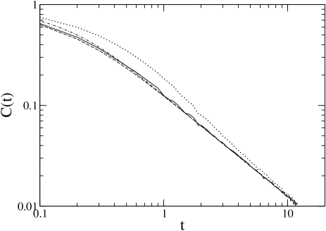
Fig.1 presents ACF for ; was calculated from the definition, by means of single trajectories evolution according to Eq.(1), for and . The equilibrium probability distribution was taken as the initial condition. The result for the larger value of agrees very well with the first term in Eq.(12) and it can be parameterized by the function
| (14) |
The existence of long tails of ACF means that the power spectrum of the process, defined by the Fourier transform as , is strongly enhanced at . The power spectrum can be obtained directly from by using the Wiener-Khinchin theorem gar : . For we get the following result:
| (15) |
Then our jumping process is characterized by the algebraic power spectrum and becomes the noise for . Overpopulation of small frequency values is due to the fact that the process is dominated by long waiting times between consecutive jumps. Such long intervals correspond to small values of , i.e. to the evolution along the axis. A quantity , which means the average of the Poissonian distribution (2), is well suited to characterize long rests. The statistics of is directly connected with the process value probability distribution and, in accordance with that, the density distribution of in the equilibrium, , can be derived from the equation . In the limit of large we obtain and this result means that the Poissonian waiting time distribution with variable jumping rate can possess, effectively, power law tails.
The jumping process with resembles a deterministic dynamical system: the Lorentz gas of periodically distributed hard disks. In this lattice a particle is elastically reflected by the discs and wanders freely among them. Free paths of the particle are infinite at directions parallel to the symmetry axes. The system is characterized by the velocity autocorrelation function with the tail , analogously to Eq.(14), and by the power spectrum . However, the long free path distribution falls faster then its stochastic counterpart, like ledous .
IV Application to the generalized Langevin equation
If a Brownian particle is driven by a stochastic force with a finite correlation time, the time evolution of the velocity obeys the generalized Langevin equation mori ; lee :
| (16) |
where is a position-dependent external potential, is a stochastic force and denotes the mass of the particle. The integro-differential equation (16) can be solved numerically for any if we apply a concrete model for the noise . In the case the Eq.(16) is manageable by Laplace transforms. We obtain the following solution:
| (17) |
where the Laplace transform of the resolvent is given by the equation
| (18) |
In the Eq.(16) the usual damping term – proportional to the velocity – which appears in the ordinary Langevin equation, has been substituted by the retarded friction in the form of a memory kernel to ensure proper characteristics of the equilibrium, namely the equation should satisfy the second fluctuation-dissipation theorem kubo . The kernel has to be proportional to the noise ACF : where is the temperature which characterizes the heat bath and is the Boltzmann constant. The introduction of memory friction changes the shape of the velocity autocorrelation function considerably: it is no longer restricted to the exponentials.
We wish to demonstrate how the process described in the preceded Sections can be applied as a model for the driving stochastic force in Eq.(16). For that purpose we choose ACF possessing the tail which characterizes e.g. the noise-induced Stark broadening frisch1 and nuclear collisions in the framework of a dynamical model sron . It can be also found in problems connected with phenomena in disordered media bou . This form of ACF is of special importance for molecular dynamics because it corresponds to the problem of scattering inside a periodic lattice zach . Let us then consider the ACF given by Eq.(14). Moreover we assume . In this case and Eq.(18) reads
| (19) |
In order to obtain the resolvent we need to inverse the above transform. Computing the usual contour integral produces the following result
| (20) |
where the constants , , and follow from the numerical evaluation of poles in the Eq.(19). The resolvent has the interpretation of the velocity autocorrelation function ,
| (21) |
R(t) falls from to negative values and then rises, approaching zero very slowly from below. The behaviour of at is determined by the integral in Eq.(20). In this limit, it becomes simpler: . Integrating over yields the integrand in the form and the integral over can be estimated kam as . The final expression reads
| (22) |
Therefore the tail of diminishes very slowly, like the tail of , and it is negative.
The velocity autocorrelation function determines the transport properties of the system: the diffusion coefficient can be expressed in terms of the Laplace transform of in the form: . Since for given by Eq.(14) , the transport is subdiffusive. We come to the same conclusion by the direct calculation of the position variance . Integrating twice over time, we get the following estimation:
| (23) |
Therefore the subdiffusion is very weak and hardly distinguishable from the normal diffusion. The same form of the anomalous diffusion has been found in a chaotic (deterministic) system gei and it has been attributed to the intermittency.
Our aim is to study the motion of the particle by a direct simulation of stochastic trajectories, assuming that the driving force in Eq.(16) is modeled by means of the stochastic process and satisfies Eq.(1). We restrict our analysis to the case . Inserting of the solution of Eq.(1) into Eq.(17) yields the two-dimensional trajectory of the particle velocity:
| (24) |
where by sampling of the consecutive jumping times we apply Eq.(2) with . Moreover, in the following we take the kernel width . A simple quantity one can evaluate from the Eq.(24) is the time dependence of the velocity variance where the average is taken
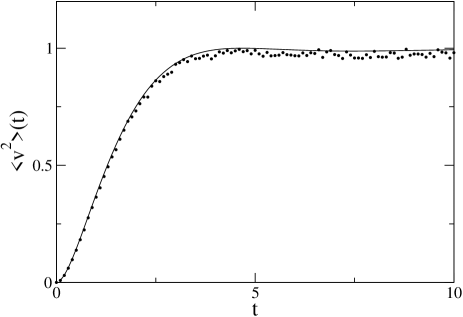
over the stationary distribution of the random force (9). Fig.2 presents this quantity, calculated with the initial condition , for and . On the other hand, the velocity variance can be derived analytically from the Eq.(24); the expression for involves only the second moment of the noise:
| (25) |
The velocity variance appears to be independent of a specific noise model and then analytical and numerical results should coincide. Indeed, Fig.2 demonstrates very good agreement of both results; they indicate the relaxation to the thermal equilibrium which is apparently reached at about uwa .
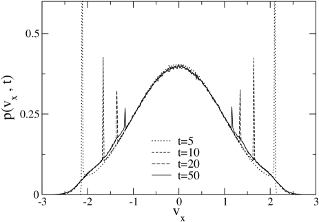
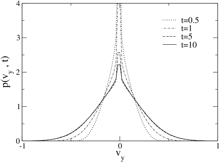
In a similar way, utilizing Eq.(24), we can determine a density distribution which means a probability that the velocity of the Brownian particle is in the interval . Fig.3 presents this distribution, corresponding to the first velocity component , for large times. The central part of the distribution is equilibrated already at but tails are not yet developed; they terminate with high and narrow peaks which originate from the initial condition . At short times (not shown in the figure) the peaks are still higher and expand gradually with time from a vicinity of the point . Full relaxation of the tails – which fall off faster than the Gaussian – to the stationary distribution is achieved at . Nevertheless, the memory about the initial condition is preserved for a very long time. The distribution of the second velocity component , presented in Fig.4, looks different; the width is much smaller and the tails show the exponential shape. A complete relaxation to stationary distribution is reached already at . The difference between the distributions for both velocity components follows from anisotropy of the function : there are no infinite waiting times corresponding to the motion in the direction.
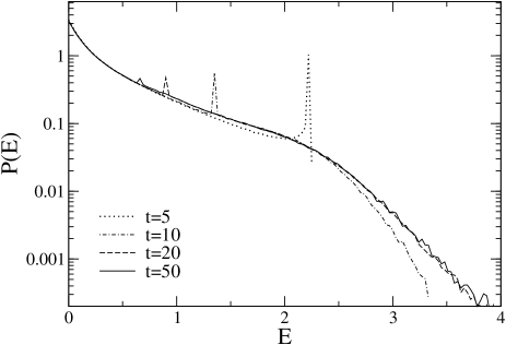
The energy spectrum of the Brownian particles deviate considerably from the Maxwellian distribution. Fig.5 presents the time evolution of the probability density distribution of the energy . At small values of the energy the curves have a cusp, whereas the tail of the distribution corresponding to the equilibrium state can be parameterized by the function . It is interesting that the probability density function which characterizes the transport dynamics in the framework of the continuous-time random walk, predicts a similar cusp for the subdiffusive motion met .
V Summary and discussion
The jumping process presented in this paper is characterized by
the jump size probability distribution and the waiting time
distribution which are correlated. The jumping rate depends on the
process value which is kept constant between consecutive jumps.
The process is Markovian and stationary, the corresponding master
equation possesses a nontrivial time-independent solution which is
completely determined by the jumping rate and which does not
depend on the jump size distribution. We have studied the process
in its two-dimensional version for jumps which do not change the
norm of the process value. The expression for ACF with power-law
tails has been derived. We have demonstrated that it is possible
to construct in a simple way a process which is a like noise.
Despite the fact that the waiting time distribution is
exponential, the intervals of constant process values can be very
long and actually algebraically distributed. This conclusion is
not surprising because the mean value of the exponential distribution
is also a stochastic variable. Then the
existence of long tails of the waiting time distribution does not
rule out a relaxation to the equilibrium.
The procedure described in the paper allows us to construct stochastic
trajectories corresponding to a wide class of power law ACF
in a simple manner. Therefore it can serve as a model of physical
phenomena and can be used as a stochastic force in the generalized Langevin
equation. We have solved this equation for an exemplary form of ACF,
, utilizing our process. Since waiting times are correlated with the
direction of the noise vector, the resulting velocity distribution exhibits a
strong anisotropy. The distribution of the first component, corresponding
to long waiting times, has rapidly falling tails
and indicates an extremely long
memory about the initial condition, despite the fact that the comprehensive
shape of the distribution equilibrates relatively fast. On the other hand,
the tails of the distribution corresponding to the second component
coincide with the standard Gaussian.
The tail of ACF is determined predominantly by the long waiting times
and then only one component of the process value is crucial for its shape.
Therefore, this component can constitute a one-dimensional counterpart of our
two-dimensional jumping process which still has the power-law ACF. This remark
is important if one requires a model of noise possessing
an arbitrary dimensionality.
References
- (1) E. W. Monroll and G. H. Weiss, J. Math. Phys. 6, 167 (1965).
- (2) R. Metzler and J. Klafter, Phys. Rep. 339, 1 (2000).
- (3) E. W. Monroll and G. H. Weiss, J. Math. Phys. 10, 753 (1969).
- (4) E. W. Monroll and H. Scher, J. Stat. Phys. 9, 101 (1973).
- (5) J.-P. Bouchaud and A. Georges, Phys. Rep. 195, 127 (1990).
- (6) S. B. Yuste and L. Acedo, Phys. Rev. E69, 031104 (2004).
- (7) V. Balakrishnan, Physica A 132, 569 (1985).
- (8) E. Barkai, R. Metzler, and J. Klafter, Phys. Rev. E 61, 132 (2000).
- (9) R. Metzler and J. Klafter, Phys. Rev. E 61, 6308 (2000).
- (10) E. Scalas, R. Gorenflo, and F. Mainardi, Phys. Rev. E 69, 011107 (2004).
- (11) A. Brissaud and U. Frisch, J. Math. Phys. 15, 524 (1974).
- (12) E. Medina, T. Hwa, M. Kardar, and Yi-Cheng Zhang, Phys. Rev. A 39, 3053 (1989).
- (13) V. Yakhot and S. A. Orszag, Phys. Rev. Lett. 57, 1722 (1986); V. Yakhot and Z.-S. She, Phys. Rev. Lett. 60, 1840 (1988).
- (14) P. Hänggi and P. Jung, Adv. Chem. Phys. 89, 229 (1995).
- (15) E. Lutz, Phys. Rev. E 64, 051106 (2001).
- (16) T. Srokowski, Phys. Rev. Lett. 85, 2232 (2000).
- (17) C. W. Gardiner, Handbook of Stochastic Methods for Physics, Chemistry and the Natural Sciences (Springer-Verlag, Berlin, 1985).
- (18) A. Kamińska and T. Srokowski, Phys. Rev. E 67, 061114 (2003).
- (19) J.P. Bouchaud and P.L. Le Doussal, J. Stat. Phys. 41, 225 (1985).
- (20) H. Mori, Prog. Theor. Phys. 33, 423 (1965); ibid 34, 399 (1965).
- (21) M. H. Lee, J. Math. Phys. 24, 2512 (1983).
- (22) R. Kubo, Rep. Prog. Phys. 29, 255 (1966).
- (23) A. Brissaud and U. Frisch, J. Quant. Spectrosc. Radiat. Transfer 11, 1767 (1971).
- (24) T. Srokowski and M. Płoszajczak, Phys. Rev. Lett. 75, 209 (1995).
- (25) A. Zacherl, T. Geisel, J. Nierwetberg, and G. Radons, Phys. Lett. A 114, 317 (1986).
- (26) T. Geisel and S. Thomae, Phys. Rev. Lett. 52, 1936 (1984).
- (27) For the kangaroo process taken as a noise model, does not reach the equilibrium value but instead it falls to zero sro .
- (28)