Fluid Invasion in Porous Media: Viscous Gradient Percolation

Abstract

We suggest that the dynamics of stable viscous invasion fronts in porous media depends on the volume capacitance of the media. At high volume capacitance, our network simulations provide numerical evidence of a scaling relation between the front width and its velocity. In the low volume capacitance regime, we derive a new effective scaling supported by network simulations and is in agreement with previous experiments on imbibition in paper and collections of glass beads.

Percolation theory has contributed much to our understanding of immiscible fluid displacement in porous media Sahimi ; Stauffer . For slow flow, randomness in capillary forces dominates and invasion percolation applies. In the presence of gravity, the local percolation probability is spatially non-uniform and gradient percolation is the standard description Hulin . Alternatively, when a viscous fluid displaces a non-viscous one, the pressure gradient also induces a gradient in the local percolation probability. The invasion front is hence expected to follow percolation geometry as well. However, the pressure field is not known apriori. This problem is therefore much more challenging and not well-understood.

Applying percolation theory, Xu, Yortsos and Salin suggested that the width of a viscous invasion front $w$ depends on its propagation velocity $v$ according to

$$w\sim v^{-\kappa}$$ (1)

where $\kappa\simeq 0.38$ in two dimensions Xu . This result is identical to that from a Buckley-Leverett type theory of Wilkinson Wilkinson although there have been other suggestions Lenormand ; Blunt . Previous network simulations lead to inconclusive results due to the limited network sizes used Xu ; Aker . In this paper, we report simulations at much larger scales using the simplest possible network models. Surprisingly, we observe two distinct scalings depending on the volume capacitance of the network defined as the volume of liquid that can be extracted from the porous medium locally per unit decrease in pressure Furuberg . At high capacitance, our simulations support the theory in Refs. Xu ; Wilkinson . At low capacitance, we obtain a different scaling in agreement with two interesting experiments on imbibition in paper Horvath and collections of glass beads Rubio .

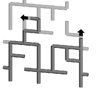
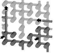
Figure 1: Snapshots of fluid invasion for networks with low (a) and high (b) volume capacitance at in-plane pipe population $p_{0}=0.53$. Wetted (dry) regions are shaded in dark (light) gray. Radii are rescaled by a factor 0.5 for clarity. Only connected pipes are shown. Arrows indicate instantaneous directions of menicus movements. Dewetting is forbidden in (a). In (b), one menicus recedes due to suction by other invaded pipes with stronger capillary forces.

Our models are based on a simple pipe network in Ref. Lam simulating the wetting of two-dimensional porous media with the bottom immersed into a liquid reservoir. We adopt a square lattice with spacing $a$ and periodic boundary conditions in the lateral direction. We define a in-plane bond population $p_{0}$ which is the probability that a bond on the square lattice is occupied by a cylindrical pipe of radius $r=0.25a$. A fraction $1-p_{0}$ of the bonds are left vacant. Given a pressure gradient $\nabla P$ along a pipe, the liquid flows according to Poiseuille’s law for viscous flow with a flux ${\pi r^{4}}\nabla P/{8\mu}$ where $\mu$ is the viscosity Sahimi . The atmospheric pressure is assumed to be zero without loss of generality. Nodes at the bottom row are directly connected to the liquid source and are also maintained at zero pressure. The pipes are simplified models of complicated fluid channels. Without strictly following the properties of realistic pipes, we assume that the capillary pressure for an advancing meniscus inside a pipe follows an uniform random distribution in the interval $[0,\Gamma_{0}]$ with $\Gamma_{0}$ being a constant. The liquid pressure behind a meniscus hence varies from $-\Gamma_{0}$ to 0. All nodes are volumeless and gravity is neglected. Air flow as well as trapping are not considered. A simple system of units in which $a=\Gamma_{0}=\mu=1$ is assumed.

Two variants of the model are considered. They differ in the volume capacitance defined as the volume of liquid extracted from the porous medium locally per unit decrease in pressure Furuberg . We first define a low capacitance network (Fig. 1(a)). In this case, we forbid any receding meniscus by assuming an ideally hysteric capillary pressure withstanding any tendency of dewetting. The liquid surface is rigid and the volume capacitance is indeed zero. We also consider a high capacitance network (Fig. 1(b)) in which receding menisci are allowed and are non-hysteric. Furthermore, an extra dangling pipe perpendicular to the lattice is connected to every node. They all have length $a$ and radius $r=0.5a$. The capillary pressure takes a random value uniformly distributed in $[0,0.3\Gamma_{0}]$. This enhance the volume capacitance at pressure around $-0.3\Gamma_{0}$ to $0$ which is the relevant range since it coincides with typical local pressures measured in wetted regions in our simulations. An increase (decrease) in the local pressure within this range activates the filling (draining) of many of these pipes resulting in the strong capacitance enhancement. We have checked that further increasing the capacitance by adding even more dangling pipes or increasing their radii give similar results. For simplicity, no new menisci can be generated by breaking any continuous column of liquid during dewetting.

We simulate fluid invasion using Euler’s method. For both models, the pressure field is first computed at the beginning of each iteration. Specifically, Poiseuille’s law and fluid conservation at all nodes leads to Kirchoff’s equations coupling the pressure at neighboring nodes. We also apply the boundary conditions that the pressure at moving and stationary menisci follows from the capillary pressure and the no flow condition respectively. The Kirchoff’s equations are then solved using successive over-relaxation method. For the low capacitance model with ideally hysteric capillarity, meniscus in a partially filled pipe may start or stop advancement depending on the calculated pressure. This alters the boundary conditions and the whole calculation is repeated until the states of motion of all menisci are consistent with the pressure field. For both models, we speed up the calculation by directly computing only the pressure at the percolation backbone. We require that the liquid influx from the source agrees with the total out-flux at the moving menisci within 1%. From the pressure, the velocities of all moving menisci are found. Their positions are then advanced over a short period in which all displacements are less than $0.1a$.

Figure 2: Log-log plot of the invasion front width $w$ against velocity $v$. The slopes of the dashed lines are -0.47 and -0.36 respectively. Inset: log-log plot of $w$ against $v\ln w$. The dashed line has a slope -0.53.

Figure 2 plots the front width $w$ against its velocity $v$ for both models at pipe population $p_{0}=0.50,0.53$ and 0.56. The lateral width of the lattice used is $L=1000a$ and all results have been averaged over 60 independent runs. Results are extracted from surface height profiles $h(x)$ measured from the liquid source which mark the highest invaded node at lateral coordinate $x$. The time derivative of the spatial and ensemble average $\bar{h}$ gives $v$ while the r.m.s. fluctuation gives $w$. The data fall nicely into straight lines in the log-log plot and verify Eq. (1). Contrary to conventional belief, there are two distinct sets of slopes averaging to $\kappa=0.47(2)$ and 0.36(2) for the low and high volume capacitance networks respectively.

Figure 3: Rescaled plots of local saturation $S$ (a), percolation probability $p$ (b), and pressure $P$ (c) against rescaled coordinate $z=(y-\bar{h})/w$. Note that $P$ requires different rescaling forms for the low and high volume capacitance cases.

To attain better insights into the problem, we now examine closely the geometry of the invasion fronts. Fronts at various locations and widths will be compared. We hence define a rescaled distance $z$ from the center of a front by $z=(y-\bar{h})/w$ where $y$ is the vertical coordinate. An important quantity is the local saturation $S(y)$ defined as the fraction of in-plane pipes which are completely invaded at height $y$. Figure 3(a) plots $S(y)/w^{D-2}$ against $z$ using the same data as in Fig. 1 where $D=91/48$ is the fractal dimension Stauffer . Values recorded near the beginning and the end of each set of simulations are plotted. Specifically, time $t$ goes from $1.8\times 10^{5}$ to $2.5\times 10^{8}$ corresponding to $w$ in between 3.1 and 32. All 12 curves collapse nicely into a single curve implying the scaling form

$$S(y)=w^{D-2}f_{S}(z)$$ (2)

where $f_{S}$ is a rescaled function. This verifies the percolation geometry of the fronts with $w$ being the correlation length Stauffer . Similarly, we define the local percolation probability $p(y)$ as the probability that an in-plane pipe connected to an invaded node is completely filled. Figure 3(b) plots $(p(y)-p_{c})/w^{-1/\nu}$ against $z$ where $\nu=4/3$ and $p_{c}=1/2$ are respectively the correlation length exponent and the percolation threshold. Good data collapse is again observed supporting

$$p(y)-p_{c}=w^{-1/\nu}f_{p}(z).$$ (3)

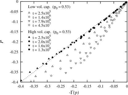
Figure 4: Plot of the average pressure $P$ against the instantaneous maximum pressure $-\Gamma(p)$ expected from the percolation probability $p$.

Data collapses for pressure in Fig. 3(c) are most interesting and will be explained after examining the relation between the local pressure and the local percolation probability. During invasion, the percolation probability at any point increases as pipes with ever lower capillary pressure are filled. Given a local percolation probability $p$, pipes with capillary pressure as low as $\Gamma(p)=(1-p/p_{0})\Gamma_{0}$ are expected to be filled. There is hence at least one instance when the pressure climbs up to instantaneous maximum value $-\Gamma(p)$. Figure 4 compares the local pressure $P$ with $-\Gamma(p)$. Only results for $p_{0}=0.53$ are shown but other values give similar findings.

At high volume capacitance, Fig. 4 shows that the pressure simply coincides with its upper bound, i.e.

$$P=-\Gamma(p)$$ (4)

Letting $P_{c}=-\Gamma(p_{c})$, it implies

$$P(y)-P_{c}~{}\sim~{}p(y)-p_{c}$$ (5)

which has been widely used in the literature Xu ; Wilkinson ; Lenormand ; Blunt ; Aker and is valid for gradient percolation Hulin . However, for viscous gradient percolation, Eq. (4) is indeed non-trivial and results from the strong damping of pressure fluctuations. Local pressure depends on the capillary pressure of the pipes under invasion. Pipes with capillary pressure in the range $[\Gamma(p),\Gamma_{0}]$ are to be invaded. The pressure is hence dominated by those with the smallest capillary pressure $\Gamma(p)$ which takes the longest time to wet. Moreover, we observe that when a pipe with a higher capillary pressure is invaded, it quickly draws liquid from neighboring pipes, especially perpendicular ones with capillary pressure close to $\Gamma(p)$. There is hence only a brief and highly localized pressure disturbance which has little impact on the average pressure. After completing the invasion, these neighbors are slowly refilled directly from the liquid reservoir and maintain the pressure roughly at $-\Gamma(p)$ again. This pressure stabilization mechanism leads to Eq. (4). Then, Eqs. (3) and (5) imply $P(y)-P_{c}=w^{-1/\nu}f_{P}(z)$. We therefore plot $(P(y)-P_{c})/w^{-1/\nu^{\prime}}$ against $z$ for the high capacitance case and is shown in Fig. 3(c) using filled symbols. We have taken $\nu^{\prime}=1.5$ for the best data collapse which is in reasonable agreement with the exact value $4/3$. The discrepancy inherits from the slight deviation from Eq. (4) as observed in Fig. 4 and results from imcomplete damping of the pressure fluctuations due to the finite volume capacitance of the network. The pressure difference $\Delta P_{H}$ across the front is hence

$$\Delta P_{H}\sim w^{-1/\nu}.$$ (6)

At low capacitance, Fig. 4 implies $P<-\Gamma(p)$ instead. Pipes with capillary pressure larger than $\Gamma(p)$ can now significantly pull down the pressure when invaded. A new analytic description of the pressure field is now presented. We first quantitatively define the front region by $z_{a}\leq z\leq z_{b}$. We take $z_{a}=-2$ since it marks the bottom of the lattice for $p_{0}=0.50$ and $z_{b}=2$ as it is where the saturation practically vanishes. We denote quantities evaluated at the boundaries by the subscripts $a$ and $b$. For $z<z_{a}$ corresponding to the bulk region, good connectivity suppresses pressure fluctuations and Eq. (4) holds approximately. In particular, the pressure at $z_{a}$ is $P_{a}=-\Gamma(p_{a})$. In contrast, the pressure fluctuates strongly at $z_{b}$ between $-\Gamma_{0}$ and $-\Gamma(p_{b})$ as pipes with capillary pressure in the range $[\Gamma(p_{b}),\Gamma_{0}]$ are invaded. With dewetting in other pipes forbidden, they draw liquid directly from the water reservoir. This leads to strong delocalized pressure fluctuations. The invasion of a pipe with capillary pressure $P_{cap}$ takes a period $\tau\sim(P_{cap}+P_{a})^{-1}$. A characteristic pressure $P_{b}$ at $z_{b}$ hence follows from the time averaged capillary pressure. Straight-forward algebra gives $P_{b}=P_{a}-\Delta P_{L}$ where

$$\Delta P_{L}=[{\Gamma_{0}-\Gamma(p_{b})}]/\ln\left[\frac{\Gamma_{0}+P_{a}}{\Gamma(p_{b})+P_{a}}\right].$$ (7)

Here $\Delta P_{L}$ represents a characteristic pressure difference across the front. We thus suggest $P(y)-P_{a}=\Delta P_{L}f_{P}(z)$. It is verified by the reasonable data collapse in Fig. 3(c) which plots $(P(y)-P_{a})/\Delta P_{L}$ against $z$ for the high capacitance case using open symbols. We have used $p_{a,b}=p_{c}+w^{-1/\nu}f_{p}(z_{a,b})$ from Eq. (3) and further assumed $f_{p}(z_{a})=0.15$ and $f_{p}(z_{b})=-0.5$ which are consistent with values read directly from Fig. 3(b).

Now, we can calculate the exponent $\kappa$ defined in Eq. (1). The permeability of the front is $k\sim w^{-\mu/\nu-1}$ where $\mu$ is the conductivity exponent Stauffer . The liquid flux across the front is then $k\Delta P_{H,L}$ for high and low capacitance respectively. However, it should equal $vS$ as well. Using also Eq. (2), we obtain $v\sim w^{\mu/\nu+D-1}\Delta P_{L,H}$. For the high capacitance model obeying Eq. (6), we arrive at Eq. (1) with

$$\kappa=\nu/(1+\mu+\nu(D-1))\simeq 0.38$$ (8)

derived previously in Refs. Xu ; Wilkinson ; Aker . Our network simulations in the high capacitance regime lead to $\kappa\simeq 0.36(2)$ giving a direct numerical support to Eq. (8).

For the low capacitance case, we apply Eq. (7) which simplifies at large $w$ to $\Delta P_{L}\sim(\ln w)^{-1}$. Therefore, Eq. (1) is replaced by

$$v\sim\frac{w^{-1/\kappa}}{\ln w}$$ (9)

with a new exponent

$$\kappa=\nu/(\mu+\nu(D-1))\simeq 0.53$$ (10)

The scaling thus admits a logarithmic correction. This is verified by the log-log plot of $w$ against $v\ln w$ in the inset of Fig. 2 which gives straight lines with the expected slope -0.53(2) for $w\gtrsim 8$. A naive measurement of $\kappa$ from a log-log plot of $w$ against $v$ disregarding the correction should lead to an effective exponent $\kappa_{e}$ in between $0.38$ and $0.53$. Using Eq. (7), we obtain $\kappa_{e}\simeq 0.46$ in good agreement with the value $0.47(2)$ directly measured from our simulations and 0.48 from imbibition experiments in Refs. Horvath ; Rubio .

We have considered extreme values of the volume capacitance. In general, networks with significant pressure fluctuations extending beyond or well-within the invasion front are at the low or high capacitance limit respectively. Networks with intermediate capacitance are therefore expected to crossover to the high capacitance regime at the large front width limit. However, from experiments, pressure fluctuations in the form of Haines jumps propagate far beyond the invasion front Furuberg . It is also known that wetting and drainage in porous media are highly hysteric. These further establish that the new low-capacitance condition is the correct experimentally relevant regime. In addition, similar to the original model in Ref. Lam , our low capacitance model can also reproduce the rich dynamical features of the invasion front in Ref. Horvath with reasonable accuracy at $p_{0}=0.53$ and will be reported elsewhere.

In conclusion, we have derived a new effective scaling relation based on viscous gradient percolation for fluid invasion fronts in porous media with low volume capacitance. This regime is characterized by realistic features including highly hysteric capillary flow and long-range propagation of pressure disturbances. The scaling is supported by large scale network simulations and agrees with previous experiments. We also show numerically that a well-known scaling theory applies only at high volume capacitance which is not supported experimentally.

We thank V.K. Horváth, L.M. Sander, J.Q. You and F.G. Shin for helpful discussions. This work was supported by HK RGC Grant No. PolyU-5191/99P.

References

- (1) M. Sahimi, Flow and transport in porous media and fractured rock, VCH (1995).
- (2) D. Stauffer and A. Aharony, Introduction to percolation theory, 2nd ed., Taylor & Francis (1994).
- (3) J.P. Hulin, E. Clément, C. Baudet, J.F. Gouyet, and M. Rosso, Phys. Rev. Lett. 61, 333 (1988).
- (4) B. Xu, Y.C. Yortsos, and D. Salin, Phys. Rev. E 57, 739 (1998).
- (5) D. Wilkinson, Phys. Rev. A 34, 1380 (1986).
- (6) R. Lenormand, Proc. R. soc. London, Ser. A 423, 159 (1989).
- (7) M. Blunt, M.J. King, and H. Scher, Phys. Rev. A 46, 7680 (1992).
- (8) E. Aker, K.J Mäløy, and Alex Hansen, Phys. Rev. E 61, 2936 (2000).
- (9) L. Furuberg, K.J. Mäløy, and J. Feder, Phys. Rev. E 53, 966 (1996).
- (10) V. K. Horváth and H. E. Stanley, Phys. Rev. E 52, 5166 (1995)
- (11) M.A. Rubio, C.A. Edwards, A. Dougherty and J.P. Gollub, Phys. Rev. Lett. 63 1685 (1989).
- (12) C.H. Lam and V.K. Horváth, Phys. Rev. Lett. 85, 1238 (2000); Phys. Rev. Lett. 86, 6047 (2001).