Linear response theory around a localized impurity in the pseudogap regime of an anisotropic superconductor: precursor pairing vs the $d$-density-wave scenario

Abstract

We derive the polarizability of an electron system in (i) the superconducting phase, with $d$-wave symmetry, (ii) the pseudogap regime, within the precursor pairing scenario, and (iii) the $d$-density-wave (dDW) state, characterized by a $d$-wave hidden order parameter, but no pairing. Such a calculation is motivated by the recent proposals that imaging the effects of an isolated impurity may distinguish between precursor pairing and dDW order in the pseudogap regime of the high-$T_{c}$ superconductors. In all three cases, the wave-vector dependence of the polarizability is characterized by an azymuthal modulation, consistent with the $d$-wave symmetry of the underlying state. However, only the dDW result shows the fingerprints of nesting, with nesting wave-vector ${\bf Q}=(\pi,\pi)$, albeit imperfect, due to a nonzero value of the hopping ratio $t^{\prime}/t$ in the band dispersion relation. As a consequence of nesting, the presence of hole pockets is also exhibited by the $({\bf q},\omega)$ dependence of the retarded polarizability.

I Introduction

Imaging of the electronic properties around an isolated nonmagnetic impurity such as Zn in the high-$T_{c}$ superconductors (HTS) has provided direct evidence of the unconventional nature of the superconducting state in the cuprates, and in particular of the $d$-wave symmetry of its order parameter below the critical temperature $T_{c}$ Pan et al. (2000); Hudson et al. (1999, 2001); Pan et al. (2001). In the underdoped regime of the HTS, various models have been proposed to describe the pseudogap state above $T_{c}$.

Several experimental results provide substantial evidence of a pseudogap opening at the Fermi level in underdoped cuprates for $T_{c}<T<T^{\ast}$, even though no unique definition of the characteristic temperature $T^{\ast}$ is possible, as it generally depends on the actual experimental technique employed (see Refs. Randeria (1999); Timusk and Statt (1999) for a review, and refs. therein). Also, the doping dependence of $T^{\ast}$ is still a matter of controversy Tallon and Loram (2001). Owing to its $d$-wave symmetry, the pseudogap has been naturally interpreted in terms of precursor superconducting pairing. In particular, the pseudogap has been associated to phase fluctuations of the order parameter above $T_{c}$ Emery and Kivelson (1995) (see Ref. Loktev et al. (2001) for a review). Within this precursor pairing scenario, the phase diagram of the HTS can be described as a crossover from Bose-Einstein condensation (in the underdoped regime) to BCS superconductivity (in the overdoped regime) Loktev et al. (2001); Randeria (1995); Andrenacci et al. (1999); Strinati (2000).

Recently, it has been proposed that many properties of the pseudogap regime may be explained within the framework of the so-called $d$-wave-density scenario (dDW) Chakravarty et al. (2001a, b); Chakravarty and Kee (2000). This is based on the idea that the pseudogap regime be characterized by a fully developed order parameter, at variance with the precursor pairing scenario, where a fluctuating order parameter is postulated. The dDW state is an ordered state of unconventional kind, and is usually associated with staggered orbital currents in the CuO₂ square lattice of the HTS Affleck and Marston (1988); Marston and Affleck (1989); Kotliar (1988); Schulz (1989). Much attention has been recently devoted to show the consistency of the dDW scenario with several experimental properties of the HTS Chakravarty et al. (2001b). These include transport properties, such as the electrical and thermal conductivities Yang and Nayak (2002); Sharapov et al. (2003) and the Hall effect Chakravarty et al. (2002); Balakirev et al. (2003), thermodynamic properties Kee and Kim (2002); Wu and Liu (2002), time symmetry breaking Kaminski et al. (2002), and angular resolved photoemission spectroscopy (ARPES) Chakravarty et al. (2003). The possible occurrence of a dDW state in microscopic models of correlated electrons has been checked in ladder networks Marston et al. (2002).

It has been recently proposed that direct imaging of the local density of states (LDOS) around an isolated impurity by means of scanning tunneling microscopy (STM) could help understanding the nature of the ‘normal’ state in the pseudogap regime Zhu et al. (2001); Wang (2002); Morr (2002); Møller Andersen (2003). The idea that an anisotropic superconducting gap should give rise to directly observable spatial features in the tunneling conductance near an impurity was suggested by Byers et al. Byers et al. (1993), whereas earlier studies Choi and Muzikar (1990) had considered perturbations of the order parameter to occur within a distance of the order of the coherence length $\xi$ around an impurity. Later, it was shown that an isolated impurity in a $d$-wave superconductor produces virtual bound states close to the Fermi level, in the nearly unitary limit Balatsky (1995). Such a quasi-bound state should appear as a pronounced peak near the Fermi level in the LDOS at the impurity site Salkola et al. (1996), as is indeed observed in Bi-2212 Pan et al. (2000) and YBCO Iavarone et al. (2002).

In the normal state, the frequency-dependent LDOS at the nearest and next-nearest neighbor sites, with respect to the impurity site, should contain fingerprints of whether the pseudogap regime is characterized by precursor pairing Kruis et al. (2001) or dDW order Wang (2002); Morr (2002). This is due to the fact that while pairing above $T_{c}$ without phase coherence is a precursor of Cooper pairing, and therefore of spontaneous breaking of U(1) gauge invariance, the dDW state can be thought as being characterized by the spontaneous breaking of particle-hole symmetry, in the same way as a charge density wave breaks pseudospin SU(2) symmetry Shen and Xie (1997). The LDOS around a nonmagnetic impurity in both the dSC, the dDW and the competing dSC+dDW phases in the underdoped regime has been actually calculated e.g. by Zhu et al. Zhu et al. (2001).

In this context, a complementary information is that provided by the polarizability $F^{\mathrm{R}}({\bf q},\omega)$ of the system, which gives a measure of the linear response of the charge density to an impurity potential. In the case of $d$-wave superconductors, it has been demonstrated that the anisotropic dependence of the superconducting order parameter on the wave-vector ${\bf q}$ gives rise to a clover-like azymuthal modulation of $F^{\mathrm{R}}({\bf q},\omega)$ along the Fermi line for a 2D system Angilella et al. (2003a).

These patterns in the ${\bf q}$ dependence of $F^{\mathrm{R}}({\bf q},\omega)$ are here confirmed also for a more realistic band for the cuprates. In addition to that, the dDW result also shows fingerprints of the ${\bf Q}=(\pi,\pi)$ nesting properties of such a state.

The paper is organized as follows. In Sec. II, we review the expression of the polarizability for the $d$-wave superconducting state (dSC) and derive that of the $d$-wave pseudogap regime, within the precursor pairing scenario (dPG). In Sec. III, we derive the polarizability for the dDW state. By allowing nonzero values of the hopping ratio $t^{\prime}/t$ in the dispersion relation Pavarini et al. (2001); Angilella et al. (2002); Angilella et al. (2003b), we will explicitly consider the case in which perfect nesting is destroyed. Such a case is relevant for the study of the dDW state, given its particle-hole character. In Sec. IV, we consider the competition of dDW order with an subdominant dSC state in the underdoping regime. In Sec. V, we present our numerical results for the polarizability in the dSC, dPG, and dDW states, both in the static limit and as a function of frequency. We eventually summarize and make some concluding remarks in Sec. VI.

II Linear response function in the dSC and dPG states

Within linear response theory, the displaced charge density $\delta\rho({\bf r})$ by a scattering potential $V({\bf r})$ in the Born approximation is given by

$$\delta\rho({\bf r})=\int V({\bf r}^{\prime})F^{\mathrm{R}}({\bf r}-{\bf r}^{\prime},E_{\mathrm{F}})d{\bf r}^{\prime},$$ (1)

which implicitly defines the linear response function $F^{\mathrm{R}}({\bf r},E_{\mathrm{F}})$ at the Fermi energy $E_{\mathrm{F}}$. Here and in the following we set the elementary charge $e=1$. Its relevance in establishing the electronic structure of isolated impurities in normal metals and alloys has been earlier emphasized by Stoddart et al. Stoddart et al. (1969); Jones and March (1986). In momentum space, Eq. (1) readily translates into $\delta\rho({\bf q})=V({\bf q})F^{\mathrm{R}}({\bf q},E_{\mathrm{F}})$, showing that, for a highly localized scattering potential in real space [$V({\bf r})=V_{0}\delta({\bf r})$, say], the Fourier transform $\delta\rho({\bf q})$ of the displaced charge is simply proportional to $F^{\mathrm{R}}({\bf q},E_{\mathrm{F}})$.

In the presence of superconducting pairing, the generalization of the linear response function is given by the density-density correlation function (polarizability) Prange (1963):

$$F({\bf q},i\omega_{\nu}) = {\mathop{\rm{Tr}}\nolimits\,}\frac{1}{\beta}\sum_{\omega_{n}}\frac{1}{N}\sum_{\bf k}\tau_{3}{\mathcal{G}}({\bf k},i\omega_{n})$$ (2)

$$\times\,\tau_{3}{\mathcal{G}}({\bf k}-{\bf q},i\omega_{n}-i\omega_{\nu})$$

where ${\mathcal{G}}({\bf k},i\omega_{n})$ is the matrix Green’s function in Nambu notation, $\beta=T^{-1}$ is the inverse temperature, $\omega_{\nu}=2\nu\pi T$ is a bosonic Matsubara frequency, $\tau_{i}$ are the Pauli matrices in spinor space, the summations are performed over the $N$ wave-vectors ${\bf k}$ of the first Brillouin zone (1BZ) and all fermionic Matsubara frequencies $\omega_{n}=(2n+1)\pi T$, and the trace is over the spin indices. Here and below we shall use units such that $\hbar=k_{\mathrm{B}}=1$ and lattice spacing $a=1$. The retarded polarizability is defined as usual in terms of the analytic continuation as $F^{\mathrm{R}}({\bf q},\omega)=F({\bf q},i\omega_{\nu}\mapsto\omega+i0^{+})$. In the normal state, Equation (2) correctly reduces to the Lindhard function for the polarizability of a free electron gas Mahan (1990).

In the following, by specifying the functional form of ${\mathcal{G}}$ in the case of pairing with and without phase coherence, we will in turn derive the explicit expression for $F$ in the superconducting phase with a $d$-wave order parameter, and in the pseudogap regime, characterized by fluctuating $d$-wave order (precursor pairing scenario).

II.1 Superconducting phase

We assume the following BCS-like Hamiltonian:

$$H_{\mathrm{dSC}}=\sum_{{\bf k}s}\xi_{\bf k}c^{\dagger}_{{\bf k}s}c_{{\bf k}s}+\sum_{{\bf k}{\bf k}^{\prime}}V_{{\bf k}{\bf k}^{\prime}}c^{\dagger}_{{\bf k}\uparrow}c^{\dagger}_{-{\bf k}\downarrow}c_{-{\bf k}^{\prime}\downarrow}c_{{\bf k}^{\prime}\uparrow},$$ (3)

where $c^{\dagger}_{{\bf k}s}$ ($c_{{\bf k}s}$) is a creation (annihilation) operator for an electron in the state with wave-vector ${\bf k}$ and spin projection $s\in\{\uparrow,\downarrow\}$ along a specified direction, and $\xi_{\bf k}=\epsilon_{\bf k}-\mu$, with $\epsilon_{\bf k}$ the single-particle dispersion relation:

$$\epsilon_{\bf k}=-2t(\cos k_{x}+\cos k_{y})+4t^{\prime}\cos k_{x}\cos k_{y},$$ (4)

where $t=0.3$ eV, $t^{\prime}/t=0.3$ are tight binding hopping parameters appropriate for the cuprate superconductors, and $\mu$ the chemical potential. In Eq. (3), $V_{{\bf k}{\bf k}^{\prime}}$ is a model potential, which we assume to be separable and attractive in the $d_{x^{2}-y^{2}}$-wave channel: $V_{{\bf k}{\bf k}^{\prime}}=-\lambda g_{\bf k}g_{{\bf k}^{\prime}}$, with $g_{\bf k}=\frac{1}{2}(\cos k_{x}-\cos k_{y})$ and $\lambda>0$. Under these assumptions, the Hamiltonian, Eq. (3), is characterized by a nonzero superconducting order parameter $\langle c_{{\bf k}\uparrow}c_{-{\bf k}\downarrow}\rangle$, leading to a nonzero $d$-wave mean-field gap $\Delta_{\bf k}=\Delta_{\circ}g_{\bf k}$ below the critical temperature $T_{c}$.

Making use of the explicit expression for the matrix Green’s function ${\mathcal{G}}_{\mathrm{dSC}}$ in the superconducting state Abrikosov et al. (1975):

$${\mathcal{G}}_{\mathrm{dSC}}({\bf k},i\omega_{n})=\frac{i\omega_{n}\tau_{0}+\xi_{\bf k}\tau_{3}+\Delta_{\bf k}\tau_{1}}{(i\omega_{n})^{2}-E_{\bf k}^{2}},$$ (5)

with $E_{\bf k}=(\xi_{\bf k}^{2}+\Delta_{\bf k}^{2})^{1/2}$ the upper branch of the superconducting spectrum and $\tau_{0}$ the identity matrix in spin space, and performing the trace over spin indices and the summation over the internal frequency Mahan (1990) in Eq. (2), we obtain the linear response function for a $d$-wave superconducting state Prange (1963):

$$F_{\mathrm{dSC}}({\bf q},i\omega_{\nu}) = \frac{1}{N}\sum_{\bf k}\left[(u_{\bf k}u_{{\bf k}-{\bf q}}-v_{\bf k}v_{{\bf k}-{\bf q}})^{2}\left(\frac{f(E_{\bf k})-f(E_{{\bf k}-{\bf q}})}{E_{\bf k}-E_{{\bf k}-{\bf q}}-i\omega_{\nu}}+\mathrm{H.c.}\right)\right.$$ (6)

$$\left.+(u_{{\bf k}-{\bf q}}v_{\bf k}+u_{\bf k}v_{{\bf k}-{\bf q}})^{2}\left(\frac{f(E_{\bf k})+f(E_{{\bf k}-{\bf q}})-1}{E_{\bf k}+E_{{\bf k}-{\bf q}}-i\omega_{\nu}}+\mathrm{H.c.}\right)\right],$$

where $u_{\bf k}^{2}=\frac{1}{2}[1+\xi_{\bf k}/E_{\bf k}]$, $v_{\bf k}^{2}=1-u_{\bf k}^{2}$ are the usual coherence factors of BCS theory, and $f(\epsilon)=(1+e^{\beta\epsilon})^{-1}$ is the Fermi function at temperature $T$. In the limit of zero external frequency and $T\to 0$, Eq. (6) reduces to the static polarizability studied in Ref. Angilella et al. (2003a) for a $d$-wave superconductor.

II.2 Pseudogap regime, within the precursor pairing scenario

In the pseudogap regime, for $T_{c}<T<T^{\ast}$, within the precursor pairing scenario Loktev et al. (2001), one assumes the existence of Cooper pairs characterized by a ‘binding energy’ $\Delta_{\bf k}$ having the same symmetry of the true superconducting gap below $T_{c}$, but no phase coherence. In other words, no true off-diagonal long range order develops, and one rather speaks of a ‘fluctuating’ order Emery and Kivelson (1995). This means that the quasiparticle spectrum $E_{\bf k}=(\xi_{\bf k}^{2}+\Delta_{\bf k}^{2})^{1/2}$ is still characterized by a pseudogap $\Delta_{\bf k}=\Delta_{\circ}g_{\bf k}$ opening at the Fermi energy with $d$-wave symmetry, but now without phase coherence. Therefore, the diagonal elements of the matrix Green’s function ${\mathcal{G}}_{\mathrm{dPG}}$ coincide with those of its superconducting counterpart, Eq. (5), while the off-diagonal, anomalous elements are null:

$${\mathcal{G}}_{\mathrm{dPG}}({\bf k},i\omega_{n})=\frac{i\omega_{n}\tau_{0}+\xi_{\bf k}\tau_{3}}{(i\omega_{n})^{2}-E_{\bf k}^{2}}.$$ (7)

The effects due to a finite lifetime of the precursor Cooper pairs can be mimicked by adding a finite imaginary energy linewidth $i\Gamma$ to the dispersion relation entering Eq. (7), or by substituting the spectral functions associated with the quasiparticle states with ‘broadened’ ones, as discussed in Appendix A. The relation between the two approaches and with analytical continuation has been discussed in Appendix A of Ref. Andrenacci and Beck (2003).

Within this precursor pairing scenario, Equation (2) in the pseudogap regime then reads:

$$F_{\mathrm{dPG}}({\bf q},i\omega_{\nu}) = \frac{1}{N}\sum_{\bf k}\left[(u_{\bf k}^{2}u_{{\bf k}-{\bf q}}^{2}+v_{\bf k}^{2}v_{{\bf k}-{\bf q}}^{2})\left(\frac{f(E_{\bf k})-f(E_{{\bf k}-{\bf q}})}{E_{\bf k}-E_{{\bf k}-{\bf q}}-i\omega_{\nu}}+\mathrm{H.c.}\right)\right.$$ (8)

$$\left.+(u_{{\bf k}-{\bf q}}^{2}v_{\bf k}^{2}+u_{\bf k}^{2}v_{{\bf k}-{\bf q}}^{2})\left(\frac{f(E_{\bf k})+f(E_{{\bf k}-{\bf q}})-1}{E_{\bf k}+E_{{\bf k}-{\bf q}}-i\omega_{\nu}}+\mathrm{H.c.}\right)\right],$$

where we are implicitly assuming $T_{c}<T<T^{\ast}$.

III Linear response function in the dDW state

The mean-field Hamiltonian for the $d$-density-wave state is Chakravarty et al. (2001a):

$$H_{\mathrm{dDW}}=\sum_{{\bf k}s}[\xi_{\bf k}c^{\dagger}_{{\bf k}s}c_{{\bf k}s}+iD_{\bf k}c^{\dagger}_{{\bf k}s}c_{{\bf k}+{\bf Q}s}],$$ (9)

where the summation is here restricted to all wave-vectors ${\bf k}$ belonging to the first Brillouin zone, ${\bf Q}=(\pi,\pi)$ is the dDW ordering wave-vector, and $D_{\bf k}=D_{\circ}g_{\bf k}$ is the dDW order parameter. As anticipated above, the dDW state is characterized by a broken symmetry and a well-developed order parameter, at variance with the precursor pairing scenario of the pseudogap regime. Such a state is associated to staggered orbital currents circulating with alternating sense in the neighboring plaquettes of the underlying square lattice. As a result, the unit cell in real space is doubled, and the Brillouin zone is correspondingly halved. At variance with other ‘density waves’, the dDW order is characterized not by charge or spin modulations, but rather by current modulations.

The nonzero, singlet order parameter $\Phi_{\bf Q}$ breaks pseudospin invariance in the particle-hole space:

$$\langle c^{\dagger}_{{\bf k}+{\bf Q}s}c_{{\bf k}s^{\prime}}\rangle=i\Phi_{\bf Q}g_{\bf k}\delta_{ss^{\prime}}.$$ (10)

Whereas it possesses $d$-wave symmetry, as expected, its imaginary value leads to the breaking of a relatively large number of symmetries, such as time reversal, parity, translation by a lattice spacing, and rotation by $\pi/2$, although the product of any two of these is preserved (see Ref. Sharapov et al. (2003) for a detailed analysis).

Introducing the spinor $\Psi_{{\bf k}s}^{\dagger}=(c^{\dagger}_{{\bf k}s}\,\,c^{\dagger}_{{\bf k}+{\bf Q}s})$, the dDW Hamiltonian, Eq. (9), can be conveniently rewritten as Yang and Nayak (2002); Sharapov et al. (2003):

$$H_{\mathrm{dDW}}={\sum_{{\bf k}s}}^{\prime}\Psi_{{\bf k}s}^{\dagger}[(\epsilon_{\bf k}^{+}-\mu)\tau_{0}+\epsilon_{\bf k}^{-}\tau_{3}+D_{\bf k}\tau_{1}]\Psi_{{\bf k}s},$$ (11)

where $\epsilon_{\bf k}^{\pm}=\frac{1}{2}(\epsilon_{\bf k}\pm\epsilon_{{\bf k}+{\bf Q}})$, and the prime restricts the summation over wave-vectors ${\bf k}$ belonging to the reduced (‘magnetic’) Brillouin zone only. Notice that $\epsilon^{\pm}_{{\bf k}+{\bf Q}}=\mp\epsilon_{\bf k}^{\pm}$. Correspondingly, the matrix Green’s function at the imaginary time $\tau$ can be defined as ${\mathcal{G}}_{\mathrm{dDW}}({\bf k},\tau)=-\langle T_{\tau}\Psi_{{\bf k}s}(\tau)\Psi^{\dagger}_{{\bf k}s}(0)\rangle$, whose inverse reads Morr (2002); Sharapov et al. (2003):

$${\mathcal{G}}_{\mathrm{dDW}}^{-1}({\bf k},i\omega_{n})=\begin{pmatrix}i\omega_{n}-\xi_{\bf k}&iD_{\bf k}\\ -iD_{\bf k}&i\omega_{n}-\xi_{{\bf k}+{\bf Q}}\end{pmatrix}.$$ (12)

In the case of perfect nesting ($t^{\prime}=0$) for the dispersion relation, Eq. (4), Sharapov et al. Sharapov et al. (2003) explicitly find

$${\mathcal{G}}_{\mathrm{dDW}}({\bf k},i\omega_{n})=\frac{(i\omega_{n}+\mu)\tau_{0}+\epsilon_{\bf k}\tau_{3}-D_{\bf k}\tau_{2}}{(i\omega_{n}+\mu)^{2}-\epsilon_{\bf k}^{2}-D_{\bf k}^{2}},$$ (13)

to be compared and contrasted with Eq. (5) for the superconducting phase. Notice, in particular, the different way the chemical potential $\mu$ enters the two expressions.

In the general case ($t^{\prime}\neq 0$), perfect nesting is lost, and we have to refer to the general form of ${\mathcal{G}}_{\mathrm{dDW}}^{-1}$, Eq. (14). One finds:

$${\mathcal{G}}_{\mathrm{dDW}}({\bf k},i\omega_{n}) = \frac{1}{(i\omega_{n}-E_{\bf k}^{+})(i\omega_{n}-E_{\bf k}^{-})}$$ (14)

$$\times\,\begin{pmatrix}i\omega_{n}-\xi_{{\bf k}+{\bf Q}}&-iD_{\bf k}\\ iD_{\bf k}&i\omega_{n}-\xi_{\bf k}\end{pmatrix},$$

where $E_{\bf k}^{\pm}=-\mu+\epsilon_{\bf k}^{+}\pm\sqrt{(\epsilon_{\bf k}^{-})^{2}+D_{\bf k}^{2}}$ are the two branches of the quasiparticle spectrum obtained by diagonalizing Eq. (9) Yang and Nayak (2002). Notice that $E_{{\bf k}+{\bf Q}}^{\pm}=E^{\pm}_{\bf k}$.

In the limit $t^{\prime}=0$, Eq. (14) correctly reduces to Eq. (13), even though it is not straightforward to express Eq. (14) in the same compact matrix notation. In the limit of perfect nesting ($t^{\prime}=0$), the dispersion relation, Eq. (4), is antisymmetric with respect to particle-hole conjugation, $\epsilon_{{\bf k}+{\bf Q}}=-\epsilon_{\bf k}$. As a result, $E_{\bf k}^{\pm}=-\mu\pm(\epsilon_{\bf k}^{2}+D_{\bf k}^{2})^{1/2}$, which is to be contrasted with the quasiparticle spectrum of the superconducting state or the pseudogap state within the precursor pairing scenario, $\pm E_{\bf k}=\pm[(\epsilon_{\bf k}-\mu)^{2}+\Delta_{\bf k}^{2}]^{1/2}$. The difference comes again from the fact that the Bogoliubov excitations in the dSC and the dPG states are Cooper pairs, while the dDW ordered state is characterized by particle-hole mixture Kee and Kim (2002); Møller Andersen (2003).

The polarizability in the dDW state is derived in Appendix B. We just quote here the final result, which can be cast in compact matrix notation as:

$$F_{\mathrm{dDW}}({\bf q},i\omega_{\nu}) = {\mathop{\rm{Tr}}\nolimits\,}\frac{1}{\beta}\sum_{\omega_{n}}\frac{1}{N}{\sum_{\bf k}}^{\prime}\kappa{\mathcal{G}}_{\mathrm{dDW}}({\bf k},i\omega_{n})$$ (15)

$$\times\,\kappa{\mathcal{G}}_{\mathrm{dDW}}({\bf k}-{\bf q},i\omega_{n}-i\omega_{\nu}),$$

where now $\kappa=\tau_{0}+\tau_{1}$, and ${\mathcal{G}}_{\mathrm{dDW}}$ is the matrix Green’s function for the dDW state, Eq. (14). Performing the frequency summation Mahan (1990), one eventually finds:

$$F_{\mathrm{dDW}}({\bf q},i\omega_{\nu})=\frac{1}{N}{\sum_{\bf k}}^{\prime}\sum_{i,j=\pm}\frac{f(E_{\bf k}^{i})-f(E_{{\bf k}-{\bf q}}^{j})}{E_{\bf k}^{i}-E_{{\bf k}-{\bf q}}^{j}-i\omega_{\nu}}.$$ (16)

IV Competition between dSC and dDW orders

In the underdoped regime, it has been predicted on phenomenological grounds that the dDW order should compete with a subdominant dSC phase Chakravarty et al. (2001a). This has been confirmed by model calculations at the mean-field level Zhu and Ting (2001); Wu and Liu (2002), showing that indeed an existing broken symmetry of dDW kind at high temperature suppresses that critical temperature for the subdominant dSC ordered phase. Recently, the competition between dDW and dSC orders has been shown to be in agreement with the unusual $T$-dependence of the restricted optical sum rule, as observed in the underdoped HTS Benfatto et al. (2003).

In order to take into account for the competition between the dSC and dDW orders at finite temperature, one has to separately consider the electron states within the two inequivalent halves of the Brillouin zone. Therefore, it is convenient to make use of the 4-components Nambu spinor $\Psi_{\bf k}^{\dagger}\equiv(\Psi_{{\bf k}\uparrow}^{\dagger}~{}~{}\Psi_{-{\bf k}\downarrow}^{\top})$, or explicitly:

$$\Psi_{\bf k}=\begin{pmatrix}c_{{\bf k}\uparrow}\\ c_{{\bf k}+{\bf Q}\uparrow}\\ c^{\dagger}_{-{\bf k}\downarrow}\\ c^{\dagger}_{-{\bf k}-{\bf Q}\downarrow}\end{pmatrix}.$$ (17)

At the mean-field level, the Hamiltonian for the competing dSC and dDW phases thus reads

$$H_{{\mathrm{dSC}}+{\mathrm{dDW}}}={\sum_{\bf k}}^{\prime}\Psi_{\bf k}^{\dagger}\hat{H}_{\bf k}\Psi_{\bf k},$$ (18)

where $\hat{H}_{\bf k}$ is the $4\times 4$ Hermitean matrix defined by

$$\hat{H}_{\bf k}=\begin{pmatrix}\xi_{\bf k}&iD_{\bf k}&\Delta_{\bf k}&0\\ -iD_{\bf k}&\xi_{{\bf k}+{\bf Q}}&0&-\Delta_{\bf k}\\ \Delta_{\bf k}^{\ast}&0&-\xi_{-{\bf k}}&iD_{-{\bf k}}\\ 0&-\Delta^{\ast}_{\bf k}&-iD_{-{\bf k}}&-\xi_{-{\bf k}-{\bf Q}}\end{pmatrix},$$ (19)

with real eigenvalues $E_{{\bf k}i}$ (here, $i=0,\ldots 3$) given by

$$E^{2}_{{\bf k}i} = \Delta_{\bf k}^{2}+D_{\bf k}^{2}-\xi_{\bf k}\xi_{{\bf k}+{\bf Q}}$$ (20)

$$+(\xi_{\bf k}+\xi_{{\bf k}+{\bf Q}})\left[\epsilon_{\bf k}^{+}-\mu\pm\sqrt{(\epsilon_{\bf k}^{-})^{2}+D_{\bf k}^{2}}\right],$$

and orthonormal eigenvectors $|{\bf k}i\rangle$ (for given ${\bf k}$ in the reduced 1BZ). It may be straightforwardly checked that $E_{{\bf k}i}$ reduces to the dSC superconducting spectrum, $\pm E_{\bf k}$, and to the dDW quasiparticle dispersion relations, $E_{\bf k}^{\pm}$, in the limits $D_{\circ}=0$ (pure dSC) and $\Delta_{\circ}=0$ (pure dDW), respectively, when the halving of the 1BZ is removed.

In the particle-hole symmetric case ($t^{\prime}=0$), making use of the nesting properties described in Sec. III, Eq. (20) simplifies as:

$$E_{{\bf k}i}=\pm\sqrt{\Delta_{\bf k}^{2}+\left(\mu\pm\sqrt{\epsilon_{\bf k}^{2}+D^{2}_{\bf k}}\right)^{2}}.$$ (21)

For $\mu=0$, the four branches of the spectrum degenerate into the Dirac cone Lee (1997); Lee and Wen (1997)

$$E_{{\bf k},0\equiv 2,1\equiv 3}=\pm\sqrt{\epsilon_{\bf k}^{2}+\Delta_{\bf k}^{2}+D^{2}_{\bf k}},$$ (22)

thus showing that the two gaps have the same role, i.e. the system may be equivalently described as a dDW or a dSC superconductor, with a $d$-wave gap $\sqrt{\Delta_{\bf k}^{2}+D^{2}_{\bf k}}$ in either case. Either a non-zero hopping ratio ($t^{\prime}/t\neq 0$) or a hole-doping away from half-filling ($\mu\neq 0$ when $t^{\prime}=0$) destroys this particular symmetry, and one has to resort to the eigenvalues $E_{{\bf k}i}$, Eq. (20).

In order to obtain the Green’s functions in the dSC+dDW case, it is useful to introduce the $4\times 4$ matrices ($i,j=0,\ldots 3$)

$$\Gamma_{ij}=\tau_{i}\otimes\tau_{j},$$ (23)

whose algebra is given by

$$\Gamma_{ij}\Gamma_{lm}=i\varepsilon_{ijk}i\varepsilon_{lmn}\Gamma_{kn},$$ (24)

where $\varepsilon_{ijk}$ is the totally antisymmetric Levi-Civita tensor, and

$$\Gamma_{33}^{\pm}=\frac{1}{2}(\Gamma_{30}\pm\Gamma_{33}).$$ (25)

Then the matrix Hamiltonian Eq. (19) takes the form

$$\hat{H}_{\bf k}=\epsilon_{\bf k}\Gamma_{33}^{+}+\epsilon_{{\bf k}+{\bf Q}}\Gamma_{33}^{-}-\mu\Gamma_{30}-D_{\bf k}\Gamma_{02}+\Delta_{\bf k}\Gamma_{13},$$ (26)

whence the inverse Green’s function (now a $4\times 4$ matrix in Nambu space) straightforwardly follows as

$${\mathcal{G}}^{-1}_{{\mathrm{dSC}}+{\mathrm{dDW}}}({\bf k},i\omega_{n})=i\omega_{n}\Gamma_{00}-\hat{H}_{\bf k}.$$ (27)

As in the dDW case, Eq. (15) (see also Appendix B), the linear response function in the dSC+dDW case can be given a compact matrix form as

$$F_{{\mathrm{dSC}}+{\mathrm{dDW}}}({\bf q},i\omega_{\nu}) = {\mathop{\rm{Tr}}\nolimits\,}\frac{1}{\beta}\sum_{\omega_{n}}\frac{1}{N}{\sum_{\bf k}}^{\prime}\hat{\kappa}{\mathcal{G}}_{{\mathrm{dSC}}+{\mathrm{dDW}}}({\bf k},i\omega_{n})$$ (28)

$$\!\!\!\!\!\!\!\times\,\hat{\kappa}{\mathcal{G}}_{{\mathrm{dSC}}+{\mathrm{dDW}}}({\bf k}-{\bf q},i\omega_{n}-i\omega_{\nu}),$$

where now the vertex matrix in the $4\times 4$ Nambu spinor space is given by

$$\hat{\kappa}=\tau_{3}\otimes\kappa=\begin{pmatrix}\tau_{0}+\tau_{1}&0\\ 0&-\tau_{0}-\tau_{1}\end{pmatrix}.$$ (29)

Finally, it can be shown that Eq. (28) also admits the following spectral decomposition, analogous to Eq. (16):

$$F_{{\mathrm{dSC}}+{\mathrm{dDW}}}({\bf q},i\omega_{\nu}) =$$

$$\!\!\!\!\!\!\!\!\!\!\!\!\!\!\!\!\!\!\!\!\!\frac{1}{N}{\sum_{\bf k}}^{\prime}\sum_{i,j}\frac{f(E_{{\bf k}i})-f(E_{{\bf k}-{\bf q}j})}{E_{{\bf k}i}-E_{{\bf k}-{\bf q}j}-i\omega_{\nu}}u_{ij}({\bf k},{\bf q}),$$

where $u_{ij}({\bf k},{\bf q})={\mathop{\rm{Tr}}\nolimits\,}(\hat{\kappa}P_{{\bf k}i}\hat{\kappa}P_{{\bf k}-{\bf q}j})$, and $P_{{\bf k}i}=|{\bf k}i\rangle\langle{\bf k}i|$ is the orthonormal projector operator on the $i$ eigenstate of the matrix Hamiltonian, Eq. (19).

V Numerical results and discussion

We have evaluated numerically the polarizability for the dPG and the dDW cases, Eqs. (8) and (16), and for the mixed dSC+dDW case, Eq. (LABEL:eq:FdSCdDW), as a function of the relevant variables. Our numerical results for the pure dSC case turn out to be very similar to the dPG case (at least over the range of variables considered below), and will not be shown here. In the dPG and in the pure dDW cases, we adopt the following set of parameters, which are believed to be relevant for the cuprate superconductors: $t=0.3$ eV, $t^{\prime}/t=0.3$, $\mu=-t$, corresponding to a hole-like Fermi line and a hole doping $\sim 14.3\%$, $\Delta_{\circ}=D_{\circ}=0.06$ eV in the dPG and in the dDW cases, respectively Chakravarty et al. (2003), and $T=100$ K.

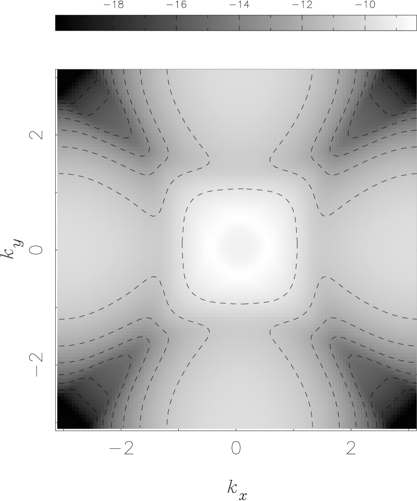
(a)

(b)

Figure 1: Static polarizability for the dPG state in momentum space, $F_{\mathrm{dPG}}({\bf q},0)$, Eq. (8) [in eV^-1, panel (a)], for $\Delta_{\circ}=0.06$ eV, $T=100$ K, and $\mu=-t=-0.3$ eV, corresponding to the hole-like Fermi line in the normal state shown in panel (b). Panel (b) also reports the special points $\Gamma=(0,0)$, $X=(\pi,0)$, $M=(\pi,\pi)$, along with the points $A$ and $B$ where the Fermi line $\xi_{\bf k}=0$ intersects the symmetry contour $\Gamma$–$X$–$M$–$\Gamma$.

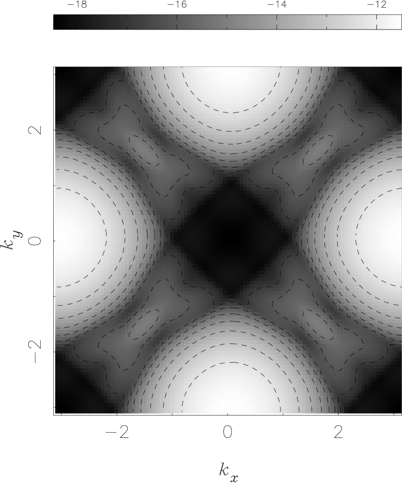
(a)

(b)

Figure 2: Static polarizability for the pure dDW state in momentum space, $F_{\mathrm{dDW}}({\bf q},0)$, Eq. (16) [in eV^-1, panel (a)], for $D_{\circ}=0.06$ eV, $T=100$ K, and $\mu=-t=-0.3$ eV, corresponding to the hole pockets $E_{\bf k}^{-}=0$ shown in panel (b). Panel (b) also reports the special points $\Gamma=(0,0)$, $X=(\pi,0)$, $M=(\pi,\pi)$, along with the points $B_{1}$ and $B_{2}$ where the line $E_{\bf k}^{-}=0$ intersects the symmetry contour $\Gamma$–$X$–$M$–$\Gamma$.

V.1 Zero external frequency

In order to make contact with earlier work Angilella et al. (2003a), we first consider the case of zero external (bosonic) frequency, $\omega_{\nu}=0$, in the time-ordered polarizabilities, Eqs. (8) and (16).

Our numerical results for the wave-vector dependence of $F({\bf q},0)$ over the 1BZ in the dPG and in the pure dDW cases are shown in Figs. 1 and 2, respectively. As a result of the $d$-wave symmetry of both the pseudogap within the precursor pairing scenario, and of the dDW order parameter, $F({\bf q},0)$ is characterized by a four-lobed pattern or azymuthal modulation Angilella et al. (2003a). However, the dDW case is also characterized by the presence of ‘hole pockets’, centered around ${\bf Q}/2=(\pi/2,\pi/2)$ and symmetry related points, due to the (albeit imperfect) nesting properties of the dDW state, with nesting vector ${\bf Q}=(\pi,\pi)$ (see Fig. 2b). Such a feature is reflected in the ${\bf q}$ dependence of $F_{\mathrm{dDW}}({\bf q},0)$, which is characterized by local maxima at the hole pockets, for the value $\mu=-t$ of the chemical potential considered here. (Other values of the chemical potentials give rise to analogous features, which are absent in the dPG case.)

Fig. 3 shows our numerical results for the static polarizability $F({\bf q},0)$ in the mixed dSC+dDW case, Eq. (LABEL:eq:FdSCdDW). Representative values of the amplitudes of the dSC and dDW order parameters have been taken as in Ref. Zhu and Ting (2001), viz. $\Delta_{\circ}=0.1t=0.03$ eV, $D_{\circ}=0.08t=0.024$ eV, at $T=0.01t\simeq 35$ K, for a particle-like Fermi line in the underdoped regime ($t=0.3$ eV, $t^{\prime}/t=0.3$, $\mu=-0.2016$ eV). Panel (b) of Fig. 3 shows the contour plot of the eigenvalue spectrum $E_{{\bf k}i}$, Eq. (20). The latter is characterized by pronounced minima near the hot spots at ${\bf Q}/2$, which evolve into cone-like nodes in the limit of pure dSC ($D_{\circ}=0$), or in the very special case $t^{\prime}=\mu=0$ [see Eq. (22)]. Accordingly, Fig. 3a for the static polarizability $F({\bf q},0)$ over the 1BZ is characterized by local maxima at the hot spots centered around ${\bf Q}/2$, as is the case in the pure dDW case (cf. Fig. 2a). Whereas the precise behavior of the static polarizability $F({\bf q},0)$ is of course determined by the actual amount of dSC+dDW mixing at a given temperature and doping, we can conclude that a sizeable dDW component manifests itself through the appearance of hole pockets centered around ${\bf Q}/2$ in the ${\bf q}$-dependence of $F({\bf q},0)$, also in the presence of a dSC condensate.

We have next evaluated the spatial dependence of $F({\bf r},0)$ (not shown), by Fourier transforming $F({\bf q},0)$ to real space. While $F({\bf r},0)$ is characterized by Friedel-like oscillations as $|{\bf r}|$ increases from the impurity site, as expected Zhu and Ting (2001); Angilella et al. (2003a), these radial, damped oscillations are superimposed by an azymuthal modulation, due to the $d$-wave symmetry of the normal state, both in the dPG and in the dDW cases. As a consequence, $F({\bf r},0)$ is characterized by a checkerboard pattern, closely related to the symmetry of the underlying square lattice, with local maxima on the nearest neighbor and local minima on the next-nearest neighbor sites. Since these features are common to both the dPG and dDW cases, the spatial dependence of the charge density oscillations is not directly helpful in distinguishing between the dPG and dDW states. However, real-space and wave-vector dependences of several quantities of interest for STM studies can be easily connected by means of Fourier transform scanning tunneling microscopy (FT-STM) techniques (see, e.g., Ref. Capriotti et al. (2003), and refs. therein). Such a technique has been proved very effective in detecting large-amplitude Friedel oscillations of the electron density on the Be(0001) Sprunger et al. (1997); Petersen et al. (1998) and Be(10$\bar{1}$0) surfaces Briner et al. (1998), and has been recently discussed in connection with experimental probes of fluctuating stripes in the HTS Kivelson et al. (2003). In particular, FT-STM experiments Sprunger et al. (1997); Petersen et al. (1998); Briner et al. (1998) have evidenced the role of correlation and reduced dimensionality in establishing such ‘giant’ Friedel oscillations in the electron density.

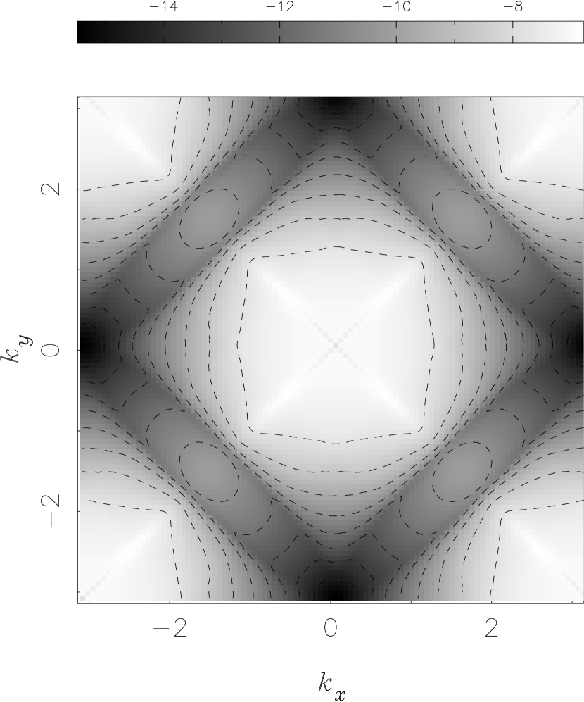
(a)

(b)

Figure 3: Static polarizability for the mixed dSC+dDW state in momentum space, $F_{{\mathrm{dSC}}+{\mathrm{dDW}}}({\bf q},0)$, Eq. (LABEL:eq:FdSCdDW) [in eV^-1, panel (a)], for $\Delta_{0}=0.1t=0.03$ eV, $D_{\circ}=0.08t=0.024$ eV, $T=0.01t\simeq 35$ K Zhu and Ting (2001), and $\mu=-0.2016$ eV, corresponding to a particle-like Fermi line closed around the $\Gamma$ point (underdoped regime). Panel (b) shows the contour plots of the eigenvalue spectrum $E_{{\bf k}i}$, Eq. 20.

V.2 Frequency dependence

We have next evaluated the frequency dependence of the retarded polarizabilities, in both the dPG and the dDW cases. Figures 4 and 5 show our numerical results for the $\omega$ dependence of $F^{\mathrm{R}}_{\mathrm{dPG}}({\bf q},\omega)$ and $F^{\mathrm{R}}_{\mathrm{dDW}}({\bf q},\omega)$, respectively. Each curve refers to either the real or the imaginary part of $F^{\mathrm{R}}({\bf q},\omega)$ as a function of $\omega$, for a fixed value of wave-vector ${\bf q}$ along the symmetry contour $\Gamma$–$X$–$M$–$\Gamma$ in the 1BZ (see Figs. 1b and 2 for its definition). While ${\bf q}$ runs along such contour, the Fermi line $\xi_{\bf k}=0$ is traversed twice (once at point $A$ along $X$–$M$ and once at $B$ along $M$–$\Gamma$, for the hole-like Fermi line considered here; see Fig. 1b), while the hole-pocket contour defined by $E_{\bf k}^{-}=0$ is traversed twice along the $M$–$\Gamma$ line (points $B_{1}\equiv B$ and $B_{2}$ in Fig. 2b).

As a consequence of the summation over ${\bf k}$ in either the full or reduced BZ in Eqs. (8) and (16), respectively, ${\mathop{\rm{Re}}\nolimits\,}F^{\mathrm{R}}({\bf q},\omega)$ is an even function of $\omega$, while ${\mathop{\rm{Im}}\nolimits\,}F^{\mathrm{R}}({\bf q},\omega)$ is an odd function of $\omega$ in both the dPG and dDW cases. Therefore, the different contributions of particle and hole states in the two cases is averaged out, and no asymmetric peaks in the $\omega$ dependence of such quantities are to be expected in the dDW case, as is the case for the local density of states Morr (2002); Møller Andersen (2003).

On the other hand, the existence of hole pockets centered around ${\bf Q}/2$ in the dDW state is clearly responsible for the different $\omega$ dependence of ${\mathop{\rm{Re}}\nolimits\,}F^{\mathrm{R}}_{\mathrm{dPG}}$ (Fig. 4a) versus ${\mathop{\rm{Re}}\nolimits\,}F^{\mathrm{R}}_{\mathrm{dDW}}$ (Fig. 5a), say, as ${\bf q}$ runs along the $\Gamma$–$X$–$M$–$\Gamma$ contours. While ${\mathop{\rm{Re}}\nolimits\,}F^{\mathrm{R}}_{\mathrm{dPG}}$ is characterized by a single relative maximum for $\omega>0$ for all wave-vectors ${\bf q}$ under consideration, ${\mathop{\rm{Re}}\nolimits\,}F^{\mathrm{R}}_{\mathrm{dDW}}$ possesses two relative maxima (or a relative maximum and a shoulder) for $\omega>0$. These two maxima tend to merge into a single one for $B_{2}\prec{\bf q}\prec B_{1}$, i.e. inside the hole pocket, and for ${\bf q}\approx A$, i.e. at the intersection of the free-particle Fermi line with the $X$–$M$ side (Fig. 5a). Likewise, the single relative maximum for $\omega>0$ in ${\mathop{\rm{Re}}\nolimits\,}F^{\mathrm{R}}_{\mathrm{dDW}}$ shifts towards larger frequencies as ${\bf q}$ runs from $\Gamma$ to $X$, is ‘diffracted’ at $A$ along the Fermi line as ${\bf q}$ runs from $X$ to $M$, and ‘bounces back’ at $B$, again along the Fermi line, as ${\bf q}$ runs from $M$ back to $\Gamma$. A similar analysis may be performed for ${\mathop{\rm{Im}}\nolimits\,}F^{\mathrm{R}}$ in the two cases (Figs. 4b and 5b).

As in the static limit, the competition of a sizeable dDW order parameter with an underlying dSC condensate does not give rise to qualitatively different results in the $\omega$-dependence of the polarizability, with respect to the pure dDW case.

One may conclude that, in both the dPG and dDW cases, the evolution with ${\bf q}$ of the features in $\omega$ dependence of $F^{\mathrm{R}}({\bf q},\omega)$ are closely related to the location of wave-vector ${\bf q}$ with respect to the Fermi line, and may therefore serve to indicate the presence of hole-pockets, as is the case for the dDW state.

(a)

(b)

Figure 4: Frequency dependence of the real [panel (a)] and imaginary parts [panel (b)] of the retarded polarizability, $F^{\mathrm{R}}({\bf q},\omega)$, in the dPG case, for wave-vector ${\bf q}$ varying along a symmetry contour $\Gamma$–$X$–$M$–$\Gamma$ in the 1BZ (see Fig. 1b). All curves have been shifted vertically for clarity, by an amount proportional to the path length from $\Gamma$ to actual wave-vector ${\bf q}$ along such symmetry contour (see right scale). Dotted line is the zero axis for $F^{\mathrm{R}}(0,\omega)$. All other parameters as in Fig. 1.

(a)

(b)

Figure 5: Same as Fig. 4, but for the dDW case. Special points in the 1BZ are as in Fig. 2b.

VI Conclusions

Motivated by recent STM experiments around a localized impurity in the HTS, we have derived the polarizability (density-density correlation function) $F({\bf q},\omega)$ for the pseudogap phase, both in the precursor pairing scenario and in the $d$-density-wave scenario. Expressions for the same function have been derived also in the underdoped regime, characterized by competing dSC+dDW orders.

In the static limit (here defined as the limit of zero external frequency for the time-ordered correlation function), the ${\bf q}$ dependence of $F({\bf q},0)$ reflects the $d$-wave symmetry of the precursor pairing ‘pseudogap’ or of the dDW order parameter, with an azymuthal modulation consistent with a clover-like pattern, as expected also for a superconductor with an isotropic band Angilella et al. (2003a). However, at variance to the dPG case, the ${\bf q}$ dependence of the static polarizability in the dDW state clearly exhibits the presence of hole pockets, due to the (albeit imperfect) nesting properties of the dDW state, with nesting vector ${\bf Q}=(\pi,\pi)$. Qualitatively similar results to the pure dDW case are obtained also in the mixed dSC+dDW, thus showing that hole pockets are a distinctive feature of dDW order. Such a behavior is confirmed by the ${\bf r}$ dependence of the static polarizability in real space. A detailed comparison with experimental data for the ${\bf r}$-dependence of the charge density displacement would of course require a much more detailed knowledge of the ${\bf q}$ dependence of the impurity potential, here crudely approximated with an $s$-wave Dirac $\delta$-function. In particular, the presence of higher momentum harmonics in the impurity potential may break the $d$-wave symmetry of the possible correlated or ordered states (dPG, dSC, dDW) here studied. Also, an extension of the present Born approximation for the impurity perturbation, e.g. to the $T$-matrix formalism, would afford a more reliable comparison with experimental results.

An analysis of the frequency dependence of the retarded polarizability $F^{\mathrm{R}}({\bf q},\omega)$ reveals that the ${\bf q}$ evolution of the features (local maxima or shoulders) in the $\omega$ dependence of this function is closely connected with the relative position of wave-vector ${\bf q}$ with respect to the Fermi line, and is therefore sensitive to the possible presence of hole pockets, as is the case for the dDW state.

Appendix A Finite lifetime effects

In order to take into account for finite lifetime effects on the linear response function for the pseudogap regime within the precursor pairing scenario, we write the diagonal elements of the matrix Green’s function as

$${\mathcal{G}}_{ii}({\bf k},i\omega_{n})=\frac{1}{2\pi}\int d\omega\frac{A_{ii}({\bf k},\omega)}{i\omega_{n}-\omega},$$ (31)

where $A_{11}({\bf k},\omega)=2\pi u_{\bf k}^{2}\delta(E_{\bf k}-\omega)$, $A_{22}({\bf k},\omega)=2\pi v^{2}_{\bf k}\delta(E_{\bf k}+\omega)$ are the appropriate spectral functions for BCS theory.

A finite energy linewidth $\Gamma$ can be attached to the energy state $E_{\bf k}$ by replacing the $\delta$-functions in the spectral functions $A_{ii}$ with broader ones, e.g. a Lorentzian function $a(\omega)=\frac{1}{\pi}\Gamma/(\omega^{2}+\Gamma^{2})$. Setting

$$A({\bf k},\omega)=2\pi[u_{\bf k}^{2}a(E_{\bf k}-\omega)+v_{\bf k}^{2}a(E_{\bf k}+\omega)],$$ (32)

in the static limit one obtains:

$$F^{\mathrm{R}}_{\mathrm{dPG}}({\bf q},\omega_{\mathrm{ext}}=0) = -\int\frac{f(\omega)-f(\omega^{\prime})}{\omega-\omega^{\prime}}$$ (33)

$$\times\,\phi({\bf q},\omega,\omega^{\prime})\,d\omega\,d\omega^{\prime},$$

where

$$\phi({\bf q},\omega,\omega^{\prime})=\frac{1}{(2\pi)^{2}}\frac{1}{N}\sum_{\bf k}A({\bf k},\omega)A({\bf k}-{\bf q},\omega^{\prime}).$$ (34)

Appendix B Polarizability for the dDW state

In order to derive the analog of the polarizability, Eq. (2), for the dDW state, we start with considering the density-density correlation function:

$$F({\bf q},\tau)=-\langle T_{\tau}\rho({\bf q},\tau)\rho(-{\bf q},0)\rangle,$$ (35)

where $\rho({\bf q},\tau)=\sum_{{\bf k}s}c^{\dagger}_{{\bf q}s}(\tau)c_{{\bf k}+{\bf q}s}(\tau)$ is the electron density operator, and $T_{\tau}$ denotes ordering with respect to the imaginary time $\tau$. Application of Wick’s theorem then yields

$$F({\bf q},\tau) = \sum_{\genfrac{}{}{0.0pt}{2}{{\bf k}{\bf k}^{\prime}}{ss^{\prime}}}\langle T_{\tau}c_{{\bf k}+{\bf q}s}(\tau)c^{\dagger}_{{\bf k}^{\prime}s^{\prime}}(0)\rangle\langle T_{\tau}c_{{\bf k}^{\prime}-{\bf q}s^{\prime}}(0)c^{\dagger}_{{\bf k}s}(\tau)\rangle$$ (36)

$$-\langle\rho({\bf q},0)\rangle\langle\rho(-{\bf q},0)\rangle,$$

the last term being a constant with respect to $\tau$, which can be neglected in Fourier transforming to the Matsubara frequency domain. In the dDW state, the contributions of terms like Eq. (10) should be explicitly considered. Therefore, we make use of the identity

$$\sum_{\bf k}f_{\bf k}={\sum_{\bf k}}^{\prime}(f_{\bf k}+f_{{\bf k}+{\bf Q}}),$$ (37)

for the summations on both ${\bf k}$ and ${\bf k}^{\prime}$ in Eq. (36), where the prime restricts the summation to wave-vectors ${\bf k}$ belonging to the reduced (magnetic) Brillouin zone. After Fourier transforming to the Matsubara frequency domain, one eventually has:

$$F_{\mathrm{dDW}}({\bf q},i\omega_{\nu}) = \frac{1}{\beta}\sum_{\omega_{n}}\frac{1}{N}{\sum_{\bf k}}^{\prime}[{\mathcal{G}}_{11}({\bf k},i\omega_{n})+{\mathcal{G}}_{12}({\bf k},i\omega_{n})$$

$$\!\!\!\!\!\!\!\!\!\!\!\!\!\!\!\!\!\!\!\!\!\!\!\!\!\!\!\!\!\!\!\!\!\!+{\mathcal{G}}_{21}({\bf k},i\omega_{n})+{\mathcal{G}}_{22}({\bf k},i\omega_{n})]$$

$$\!\!\!\!\!\!\!\!\!\!\!\!\!\!\!\!\!\!\!\!\!\!\!\!\!\!\!\!\!\!\!\!\!\!\!\!\!\!\!\!\times\,[{\mathcal{G}}_{11}({\bf k}-{\bf q},i\omega_{n}-i\omega_{\nu})+{\mathcal{G}}_{12}({\bf k}-{\bf q},i\omega_{n}-i\omega_{\nu})$$

$$\!\!\!\!\!\!\!\!\!\!\!\!\!\!\!\!\!\!\!\!\!\!\!\!\!\!\!\!\!\!\!\!\!\!+{\mathcal{G}}_{21}({\bf k}-{\bf q},i\omega_{n}-i\omega_{\nu})+{\mathcal{G}}_{22}({\bf k}-{\bf q},i\omega_{n}-i\omega_{\nu})],$$

where ${\mathcal{G}}_{ij}$ are the entries of ${\mathcal{G}}_{\mathrm{dDW}}({\bf k},i\omega_{n})$ in Eq. (14). The last expression can then be cast into the compact matrix form, Eq. (15), by introducing the constant auxiliary matrix $\kappa=\tau_{0}+\tau_{1}=\begin{pmatrix}1&1\\ 1&1\end{pmatrix}$. Equation (LABEL:eq:app:FdDW) simplifies further, by observing that ${\mathcal{G}}_{12}=-{\mathcal{G}}_{21}$ and that ${\mathcal{G}}_{11}+{\mathcal{G}}_{22}=(i\omega_{n}-E_{\bf k}^{+})^{-1}+(i\omega_{n}-E_{\bf k}^{-})^{-1}$.

References

- Pan et al. (2000) S. H. Pan, E. W. Hudson, K. M. Lang, H. Eisaki, S. Uchida, and J. C. Davis, Nature 403, 746 (2000).
- Hudson et al. (1999) E. W. Hudson, S. H. Pan, A. K. Gupta, K. W. Ng, and J. C. Davis, Science 285, 88 (1999).
- Hudson et al. (2001) E. W. Hudson, K. M. Lang, V. Madhavan, S. H. P. H. Eisaki, S. Uchida, and J. C. Davis, Nature 411, 920 (2001).
- Pan et al. (2001) S. H. Pan, J. P. O’Neal, R. L. Badzey, C. Chamon, H. Ding, J. R. Engelbrecht, Z. Wang, H. Eisaki, S. Uchida, A. K. Guptak, et al., Nature 413, 282 (2001).
- Randeria (1999) M. Randeria, in Proceedings of the CXXXVI International School of Physics “E. Fermi” on “Models and phenomenology for conventional and high-temperature superconductivity”, edited by G. Iadonisi, R. J. Schrieffer, and M. L. Chiofalo (IOS, Amsterdam, 1999), preprint cond-mat/9710223.
- Timusk and Statt (1999) T. Timusk and B. Statt, Rep. Prog. Phys. 62, 61 (1999).
- Tallon and Loram (2001) J. L. Tallon and J. W. Loram, Physica C 349, 53 (2001).
- Emery and Kivelson (1995) V. J. Emery and S. A. Kivelson, Nature 374, 434 (1995).
- Loktev et al. (2001) V. M. Loktev, R. M. Quick, and S. G. Sharapov, Phys. Rep. 349, 1 (2001).
- Randeria (1995) M. Randeria, in Bose Einstein Condensation, edited by A. Griffin, D. Snoke, and S. Stringari (Cambridge University Press, Cambridge, 1995), p. 355.
- Andrenacci et al. (1999) N. Andrenacci, A. Perali, P. Pieri, and G. C. Strinati, Phys. Rev. B 60, 12410 (1999).
- Strinati (2000) G. C. Strinati, Phys. Essays 13, 427 (2000).
- Chakravarty et al. (2001a) S. Chakravarty, R. B. Laughlin, D. K. Morr, and C. Nayak, Phys. Rev. B 63, 094503 (2001a).
- Chakravarty et al. (2001b) S. Chakravarty, H. Kee, and C. Nayak, Int. J. Mod. Phys. B 15, 2901 (2001b).
- Chakravarty and Kee (2000) S. Chakravarty and H.-Y. Kee, Phys. Rev. B 61, 14821 (2000).
- Affleck and Marston (1988) I. Affleck and J. B. Marston, Phys. Rev. B 37, 3774 (1988).
- Marston and Affleck (1989) J. B. Marston and I. Affleck, Phys. Rev. B 39, 11538 (1989).
- Kotliar (1988) G. Kotliar, Phys. Rev. B 37, 3664 (1988).
- Schulz (1989) H. Schulz, Phys. Rev. B 39, 2940 (1989).
- Yang and Nayak (2002) X. Yang and C. Nayak, Phys. Rev. B 65, 064523 (2002).
- Sharapov et al. (2003) S. G. Sharapov, V. P. Gusynin, and H. Beck, Phys. Rev. B 67, 144509 (2003).
- Chakravarty et al. (2002) S. Chakravarty, C. Nayak, S. Tewari, and X. Yang, Phys. Rev. Lett. 89, 277003 (2002).
- Balakirev et al. (2003) F. F. Balakirev, J. B. Betts, A. Migliori, S. Ono, Y. Ando, and G. S. Boebinger, Nature 424, 912 (2003).
- Kee and Kim (2002) H.-Y. Kee and Y. B. Kim, Phys. Rev. B 66, 012505 (2002).
- Wu and Liu (2002) C. Wu and W. V. Liu, Phys. Rev. B 66, R020511 (2002).
- Kaminski et al. (2002) A. Kaminski, S. Rosenkranz, H. M. Fretwell, J. C. Campuzano, Z. Li, H. Raffy, W. G.Cullen, H. You, C. G. Olson, C. M. Varma, et al., Nature 416, 610 (2002).
- Chakravarty et al. (2003) S. Chakravarty, C. Nayak, and S. Tewari, Phys. Rev. B 68, R100504 (2003).
- Marston et al. (2002) J. B. Marston, J. O. Fjærestad, and A. Sudbø, Phys. Rev. Lett. 89, 056404 (2002).
- Zhu et al. (2001) J. Zhu, W. Kim, C. S. Ting, and J. P. Carbotte, Phys. Rev. Lett. 87, 197001 (2001).
- Wang (2002) Q. Wang, Phys. Rev. Lett. 88, 057002 (2002).
- Morr (2002) D. K. Morr, Phys. Rev. Lett. 89, 106401 (2002).
- Møller Andersen (2003) B. Møller Andersen, Phys. Rev. B 68, 094518 (2003).
- Byers et al. (1993) J. M. Byers, M. E. Flatté, and D. J. Scalapino, Phys. Rev. Lett. 71, 3363 (1993).
- Choi and Muzikar (1990) E. S. Choi and P. Muzikar, Phys. Rev. B 41, 1812 (1990).
- Balatsky (1995) A. V. Balatsky, Phys. Rev. B 51, 15547 (1995).
- Salkola et al. (1996) M. I. Salkola, A. V. Balatsky, and D. J. Scalapino, Phys. Rev. Lett. 77, 1841 (1996).
- Iavarone et al. (2002) M. Iavarone, M. Salluzzo, R. Di Capua, M. G. Maglione, R. Vaglio, G. Karapetrov, W. K. Kwok, and G. Crabtree, Phys. Rev. B 65, 214506 (2002).
- Kruis et al. (2001) H. V. Kruis, I. Martin, and A. V. Balatsky, Phys. Rev. B 64, 054501 (2001).
- Shen and Xie (1997) S. Shen and X. C. Xie, Physica B 230-232, 1061 (1997), also available as preprint cond-mat/9507075.
- Angilella et al. (2003a) G. G. N. Angilella, F. E. Leys, N. H. March, and R. Pucci, J. Phys. Chem. Solids 64, 413 (2003a).
- Pavarini et al. (2001) E. Pavarini, I. Dasgupta, T. Saha-Dasgupta, O. Jepsen, and O. K. Andersen, Phys. Rev. Lett. 87, 047003 (2001).
- Angilella et al. (2002) G. G. N. Angilella, E. Piegari, and A. A. Varlamov, Phys. Rev. B 66, 014501 (2002).
- Angilella et al. (2003b) G. G. N. Angilella, R. Pucci, A. A. Varlamov, and F. Onufrieva, Phys. Rev. B 67, 134525 (2003b).
- Stoddart et al. (1969) J. C. Stoddart, N. H. March, and M. J. Stott, Phys. Rev. 186, 683 (1969).
- Jones and March (1986) W. Jones and N. H. March, Theoretical Solid-State Physics. Non-equilibrium and Disorder, vol. 2 (Dover, New York, 1986).
- Prange (1963) R. E. Prange, Phys. Rev. 129, 2495 (1963).
- Mahan (1990) G. D. Mahan, Many-Particle Physics (Plenum Press, New York and London, 1990), 2nd ed.
- Abrikosov et al. (1975) A. A. Abrikosov, L. P. Gorkov, and I. E. Dzyaloshinski, Methods of Quantum Field Theory in Statistical Physics (Dover, New York, 1975).
- Andrenacci and Beck (2003) N. Andrenacci and H. Beck, … …, … (2003), preprint cond-mat/0304084.
- Zhu and Ting (2001) J. Zhu and C. S. Ting, Phys. Rev. Lett. 87, 147002 (2001).
- Benfatto et al. (2003) L. Benfatto, S. G. Sharapov, and H. Beck, … …, … (2003), preprint cond-mat/0305276.
- Lee (1997) P. A. Lee, Science 277, 50 (1997).
- Lee and Wen (1997) P. A. Lee and X. G. Wen, Phys. Rev. Lett. 78, 4111 (1997).
- Capriotti et al. (2003) L. Capriotti, D. J. Scalapino, and R. D. Sedgewick, Phys. Rev. B 68, 014508 (2003).
- Sprunger et al. (1997) P. T. Sprunger, L. Petersen, E. W. Plummer, E. Lægsgaard, and F. Besenbacher, Science 275, 1764 (1997).
- Petersen et al. (1998) L. Petersen, P. T. Sprunger, P. Hofmann, E. Lægsgaard, B. G. Brines, M. Doering, H. Rust, and E. W. Plummer, Phys. Rev. B 57, R6858 (1998).
- Briner et al. (1998) B. G. Briner, P. Hofmann, M. Doering, H. Rust, E. W. Plummer, and A. M. Bradshaw, Phys. Rev. B 58, 13931 (1998).
- Kivelson et al. (2003) S. A. Kivelson, I. P. Bindloss, E. Fradkin, V. Oganesyan, J. M. Tranquada, A. Kapitulnik, and C. Howald, Rev. Mod. Phys. 75, 1201 (2003).