Influence of long-range correlated quenched disorder on the adsorption of long flexible polymer chains on a wall.

Abstract

The process of adsorption on a planar wall of long-flexible polymer chains in the medium with quenched long-range correlated disorder is investigated. We focus on the case of correlations between defects or impurities that decay according to the power-low $x^{-a}$ for large distances $x$, where ${\bf x}=({\bf r},z)$. Field theoretical approach in $d=4-\epsilon$ and directly in $d=3$ dimensions up to one-loop order for the semi-infinite $|\phi|^{4}$ m-vector model (in the limit $m\to 0$) with a planar boundary is used. The whole set of surface critical exponents at the adsorption threshold $T=T_{a}$, which separates the nonadsorbed region from the adsorbed one is obtained. Moreover, we calculate the crossover critical exponent $\Phi$ and the set of exponents associated with them. We perform calculations in a double $\epsilon=4-d$ and $\delta=4-a$ expansion and also for a fixed dimension $d=3$, up to one-loop order for different values of the correlation parameter $2<a\leq 3$.

The obtained results indicate that for the systems with long-range correlated quenched disorder the new set of surface critical exponents arises. All the surface critical exponents depend on $a$. Hence, the presence of long-range correlated disorder influences the process of adsorption of long-flexible polymer chains on a wall in a significant way.

I Introduction

Universal properties of long-flexible polymer chains change when small amount of long-range correlated quenched disorder is introduced into an infinite medium Blavatska01 ; Holovatch01 . The correlated defects (i.e. regions that cannot be occupied by the chain) may occur, for example, in a porous medium or in a disordered sponge-like structure formed by lipid membranes in biological systems. Intuitively, if the correlations between the defects and/or impurities decay sufficiently slowly, then the chain has to go around large correlated regions, and effectively occupies larger space, with the defects contained inside the region occupied by the coil. As a result, the polymer swells. If, however, the range of correlations is very large, then the polymer may be trapped between the walls of defects (i.e. the probability of going beyond the defected region is low), and this may lead to a collapsed state. These heuristic arguments suggest that the polymer either swells or collapses, depending on the range of correlations between the defects or impurities. Indeed, recent results agree with the intuitive expectations Blavatska01 ; Holovatch01 . For different ranges of correlations (i.e. different values of $a$ for the power-law decay of correlations $1/x^{a}$) the swelling of the polymer is described by different dependencies of the radius of gyration on the number of monomers. Finally, for $a<2.3$ Blavatska01 ; Holovatch01 a first-order transition to a collapsed state was found Blavatska01 ; Holovatch01 .

Motivated by the above results we focus our attention on the effect of the presence of a small amount of long-range correlated quenched disorder in the bulk on the adsorption of long-flexible polymer chains on a planar surface forming the system boundary. In real systems different kinds of defects and impurities may be localized inside the bulk or at the boundary. As was found in Ref.DN89 , introducing into the system short-range correlated random quenched surface disorder is irrelevant for critical behavior, but long-range correlated quenched surface disorder with $g(r)\sim 1/r^{a}$ can be relevant if $a<d-1$, and is irrelevant if $a\geq d-1$. The question how the adsorption phenomena of long flexible polymer chains depend on the presence of long-range-correlated quenched disorder in the bulk remains open, however. New universality class characterizing the polymer in the presence of long-range correlated disorder indicates that the critical exponents describing the properties of the polymer chain near the wall should assume different values than in the pure system. The purpose of this work is a determination of the surface critical exponents to first order in perturbation expansion, in order to gain information about a qualitative change of adsorption of the chains when the range of correlations between the defects in the bulk increases (i.e., $a$ is decreased).

Long flexible polymer chains in a good solvent are perfectly described by a model of self-avoiding walks (SAW) on a regular lattice Cloizeaux . Their scaling properties in the limit of an infinite number of steps $N$ may be derived by a formal $m\to 0$ limit of the $O(m)$ vector model at its critical point deGennes . The average square end-to-end distance, the number of configurations with one end fixed and with both ends fixed at the distance $x=\sqrt{({\vec{x}}_{A}-{\vec{x}}_{B})^{2}}$ exhibit the following asymptotic behavior in the limit $N\to\infty$

$$<R^{2}>\sim N^{2\nu},\quad\quad\quad Z_{N}\sim q^{N}N^{\gamma-1},\quad\quad\quad Z_{N}(x)\sim q^{N}N^{-(2-\alpha)},$$ (1)

respectively. $\nu$, $\gamma$ and $\alpha$ are the universal correlation length, susceptibility and specific heat critical exponents for the $m=0$ model, $d$ is the space dimensionality, $q$ is a non universal fugacity. $1/N$ plays a role of a critical parameter analogous to the reduced critical temperature in magnetic systems.

When the polymer solution is in contact with a solid substrate (or with vapor), then the monomers interact with the surface (or their chemical potential at the interface is different than in the bulk). At sufficiently low temperatures, $T<T_{a}$, the attraction between the monomers and the surface leads to an adsorbed state, where a finite fraction of the monomers is attached to the system boundary. Deviation from the adsorption threshold, $c\propto(T-T_{a})/T_{a})$, changes sign at the transition between the adsorbed ($c<0$) and the nonadsorbed state ($c>0$) and it plays a role of a second critical parameter. The adsorption threshold for infinite chains, where $1/N\to 0$ and $c\to 0$ is a multicritical phenomenon. We shall assume that the solution of polymer chains is sufficiently dilute, so that interchain interactions and overlapping between different chains can be neglected, and it is sufficient to consider surface effects for configurations of a single chain. For pure solvents the investigation of adsorption phenomena of long-flexible polymer chains on a surface was a subject of a series of works (for the sake of brevity we notice only few of them deGennes ; EKB82 ; eisenriegler:83 ; Eisenriegler ; HG94 ; SKG99 ; SGK01 ; RDGKS02 ; ZLB90 ). The polymer adsorption on a wall in the limit of an infinite chain is closely related to surface critical phenomena in the $m$ - vector model of a magnet in a semi-infinite geometry in the limit $m\to 0$ G76 ; deGennes ; Barber . Based on the above analogy, Eisenriegler and co-workers EKB82 ; eisenriegler:83 ; Eisenriegler described the scaling properties of long chains near a wall on the basis of the results of the field theory developed for semi-infinite magnetic systems in Ref.DD81 ; DD83 ; D86 . Surface multicritical phenomena in dilute polymer systems (at $T=T_{a}$ and $N\to\infty$) correspond to the special transition in semiinfinte magnets. The special transition ($c=0$) is characterized by one additional independent surface critical exponent $\eta_{\parallel}$, which characterizes critical correlations in directions parallel to the surface. The whole set of the other surface critical exponents can be obtained on the basis of $\eta_{\parallel}$ and the bulk critical exponents $\nu$ and $\eta$ with the help of surface scaling relations. The crossover critical exponent $\Phi$ characterizes the crossover behavior between the special and ordinary transitions ($c\neq 0$). The latter exponent is related to the length scale eisenriegler:83 ; Eisenriegler ,

$$\xi_{c}\sim|c|^{-\nu/\Phi},$$ (2)

associated with the parameter $c$. In the polymer problem the length $\xi_{c}$ can be interpreted as the distance from the surface up to which the properties of the polymer depend on the value of $c$, not only on its sign. The remaining, bulk length scales are the average end-to-end distance $\xi_{R}=\sqrt{<R^{2}>}\sim N^{\nu}$ and the microscopic length $l$ – the effective monomer linear dimension. Near the multicritical point the only relevant lengths are $\xi_{R}\to\infty$ and $\xi_{c}\to\infty$, and the properties of the system depend on the ratio $\xi_{R}/\xi_{c}$. In the asymptotic scaling regime the universal physical quantities $X(N,c)$ and $Y(z;N,c)$ assume the scaling forms

$$X(N,c)=N^{a_{X}}X^{s}_{\pm}\big{(}\xi_{R}/\xi_{c}\big{)},\hskip 28.45274ptY(z;N,c)=N^{a_{Y}}Y^{s}_{\pm}\big{(}z/\xi_{R},\xi_{R}/\xi_{c}\big{)},$$ (3)

where $X^{s}_{\pm}$ and $Y^{s}_{\pm}$ denote the scaling functions with the subscripts $+$ and $-$ corresponding to $c>0$ and $c<0$ respectively. The characteristic length ratio is $(\xi_{R}/\xi_{c})^{\Phi/\nu}\sim|c|N^{\Phi}$, where $cN^{\Phi}$ is the standard scaling variable EKB82 . The exponents $a_{X}$ and $a_{Y}$ assume different values for different quantities $X$ and $Y$. Let us first consider the mean square end-to-end distance for one end attached to the surface and the other one free. In the semi-infinite system the translational invariance is broken, and the parallel $<R^{2}_{\parallel}>$ and perpendicular $<R^{2}_{\perp}>$ parts of the average end-to-end distance $<R^{2}>=<R^{2}_{\perp}+R^{2}_{\parallel}>$ should be distinguished. For $<R^{2}_{\perp}>^{1/2}$ the exponent in the scaling form (3) is $a_{X}=\nu$ and the corresponding scaling functions assume the form $\sim const$ for $c\geq 0$ and $\sim 1/y$ for $c<0$, where $y=\xi_{R}/\xi_{c}$ EKB82 . Thus, for the adsorbed state and for $N\to\infty$ the length associated with $c$ describes the thickness $\xi$ of the adsorbed layer,

$$\xi=<R^{2}_{\perp}>^{1/2}\sim\xi_{c}\hskip 28.45274ptc<0.$$ (4)

This thickness diverges for $c=1/N=0$ and for finite negative values of $c$ remains finite for an infinite chain. For $c\geq 0$ the asymptotic behavior of the mean distance of the free end from the other end attached to the surface is

$$<R^{2}_{\perp}>^{1/2}\sim N^{\nu}\hskip 28.45274ptc\geq 0,$$ (5)

i.e it has the same asymptotic behavior as in the bulk. The asymptotic scaling form of $<R^{2}_{\parallel}>^{1/2}$ for $c<0$ is $<R^{2}_{\parallel}>^{1/2}\sim|c|^{(\nu^{d-1}-\nu)/\Phi}N^{\nu^{d-1}}$, where $\nu^{d-1}$ is the correlation exponent in $d-1$ dimensions. For $c\geq 0$ the scaling form of $<R^{2}_{\parallel}>^{1/2}$ is given by Eq. (5), i.e. it is also the same as in the bulk.

For the fraction of monomers at the surface, $N_{1}/N$, the following asymptotic behavior has been found for $N\to\infty$ EKB82 ; Eisenriegler ,

$$N_{1}/N\sim\left\{\begin{array}[]{lll}|c|^{(1-\Phi)/\Phi}&\;\;\mbox{if}&\;\;\;\mbox{$c<0$}\\ N^{\Phi-1}&\;\;\mbox{if}&\;\;\;\mbox{$c=0$}\\ (cN)^{-1}&\;\;\mbox{if}&\;\;\;\mbox{$c>0$}\end{array}\right..$$ (9)

Hence, for $N\to\infty$ and for finite, negative values of $c$, $N_{1}/N$ is finite, but for $c\geq 0$ $N_{1}/N\to 0$ for $N\to\infty$. The thickness of the adsorbed layer is closely related to the fraction of monomers at the surface $N_{1}/N$ EKB82 ; Eisenriegler , since the more monomers are fixed at the wall, the smaller the region occupied by the remaining monomers. In particular, for weakly adsorbed phase ($c<0$ and $|c|\ll 1$) we find $N_{1}/N\sim\xi^{-(1-\Phi)/\nu}$.

The scaling behavior is also obeyed by the mean number of the free ends in the layer between $z$ and $z+dz$, which is proportional to the partition function of a chain with one end fixed at ${\bf x}_{A}=({\bf r}_{A},z)$ and the other end free, $Z_{N}(z)$. The density of monomers in a layer at the distance $z$ from the wall to which one end of the polymer is attached, $M_{N}^{\lambda}(z)$ scales according to Eq. (3) as well. For the above quantities the exponent $a_{Y}$ in (3) is $\gamma-1$ and $\gamma_{1}-\nu$ respectively. Short-distance behavior ($l\ll z\ll\xi_{R}$) of the two quantities right at the threshold ($c=0$) is

$$Z_{N}(z)\sim z^{(\gamma-\gamma_{1})/\nu}N^{\gamma_{1}-1}$$ (10)

and

$$M_{N}^{\lambda}(z)\sim z^{-1+(1-\Phi)/\nu}N^{\gamma_{1}-1+\Phi}.$$ (11)

$\gamma_{1}$ as well as the whole set of the surface critical exponents can be obtained from $\eta_{\parallel}$ and $\Phi$ through scaling relations (see the Appendix). The remaining quantities characterizing the adsorption process are described in detail in Ref.EKB82 ; Eisenriegler .

Taking into account the results of ref. Blavatska01 ; Holovatch01 we conclude that for $c\geq 0$ the polymer with one end attached to the surface swells as in the bulk when $a$ decreases (see (5)). However, in order to determine the effect of the long-range correlated disorder on the adsorption of the polymer right at the threshold (see (10) and (11)) or in the crossover region (see (2), (4) and (9)) it is necessary to find the dependence of the surface critical exponents on $a$.

In the next section the model is briefly described. In sec.III the surface multicritical behavior of the system with long-range correlated disorder is outlined. The results of sec. III enable us to obtain in sec. IV the surface critical exponents to first order in the perturbation expansion. Final section contains a brief discussion of the results.

II the model

When a disorder is introduced into an infinite magnetic system, the Landau-Ginzburg-Wilson Hamiltonian deGennes assumes the form

$$H=\int_{V}d^{d}x[\frac{1}{2}\mid\nabla\vec{\phi}\mid^{2}+\frac{1}{2}(\mu_{0}^{2}+\delta\tau({\bf{x}}))\mid\vec{\phi}\mid^{2}+\frac{1}{4!}v_{0}(\vec{\phi}^{2})^{2}],$$ (12)

where $\vec{\phi}(x)$ is an $m$-vector field with the components $\phi_{i}(x)$, $i=1,...,m$. Here $\mu_{0}^{2}$ is the ”bare mass”, which in the case of a magnet corresponds to the reduced temperature. The inhomogeneities in the system cause local deviations from the average value of the transition temperature, and $\delta\tau({\bf{x}})$ represents the quenched random-temperature disorder, with $<\delta\tau({\bf{x}})>=0$ and

$$\frac{1}{8}<\delta\tau({\bf{x}})\delta\tau({\bf{x}}^{\prime})>=g(\mid{\bf{x}}\mid),$$ (13)

where angular brackets $<...>$ denote configurational averaging over quenched disorder. Following Refs.Blavatska01 ; Holovatch01 we assume that the pair correlation function $g(\mid{\bf{x}}\mid)$ falls off with the distance as

$$g(\mid{\bf{x}}\mid)\sim\frac{1}{x^{a}}$$ (14)

for large ${\bf{x}}=({\bf{r}},z)$, where $a$ is a constant and $x=\mid\bf{x}\mid$. The Fourier-transform ${\tilde{g}}(k)$ of $g(x)$ for small $k$ is

$${\tilde{g}}(k)\sim u_{0}+w_{0}\mid k\mid^{a-d}.$$ (15)

This corresponds to the so-called long-range-correlated ”random-temperature” disorder. In the case of random uncorrelated point-like (or short-range-correlated) disorder the site-occupation correlation function is $g(x)\sim\delta(x)$ and its Fourier-transform assumes the simple form

$${\tilde{g}}(k)\sim u_{0}.$$ (16)

Applying the replica method in order to average the free energy over different configurations of the quenched disorder, it is possible to construct an effective Hamiltonian of the $|\phi|^{4}$ $m$ -vector model with a long-range-correlated disorder

$$H_{eff} = \sum_{\alpha=1}^{n}\int_{V}d^{d}x[\frac{1}{2}\mid\nabla\vec{\phi}_{\alpha}\mid^{2}+\frac{1}{2}\mu_{0}^{2}\vec{\phi}_{\alpha}^{2}+\frac{1}{4!}v_{0}(\vec{\phi}_{\alpha}^{2})^{2}$$ (17)

$$-\sum_{\alpha,\beta=1}^{n}\int d^{d}x_{1}d^{d}x_{1}^{{}^{\prime}}g(\mid x_{1}-x_{1}^{{}^{\prime}}\mid)\vec{\phi}_{\alpha}^{2}(x_{1})\vec{\phi}_{\beta}^{2}(x_{1}^{{}^{\prime}}).$$

Here Greek indices denote replicas, and the replica limit $n\to 0$ is implied. If $a\geq d$, then the $w_{0}$ term is irrelevant. This corresponds to random uncorrelated point-like disorder (or short-range-correlated random disorder). As noticed by Kim Kim , in this case in the limit $m,n\to 0$ both $v_{0}$ and $u_{0}$ terms are of the same symmetry. It indicates that a weak quenched uncorrelated disorder is irrelevant for SAWs Harris . If, on the other hand, $a<d$, the term $w_{0}k^{a-d}$ is relevant for the critical behavior at $k\to 0$, and the long-range-correlated disorder is relevant for SAWs (see Blavatska01 ; Holovatch01 ). The limit $m\to 0$ of this model can be interpreted as a model of long-flexible polymer chains in a disordered medium Blavatska01 ; Holovatch01 .

The presence of a hard wall leads to a modification of the interactions in the near-surface layer. Thus, in the semi-infinite system there should be additional, surface contribution to the Hamiltonian. The effective Hamiltonian of the semi-infinite $|\phi|^{4}$ $m$-vector model with long-range-correlated disorder in this case is

$$H_{eff} = \sum_{\alpha=1}^{n}\int_{V}d^{d}x[\frac{1}{2}\mid\nabla\vec{\phi}_{\alpha}\mid^{2}+\frac{1}{2}\mu_{0}^{2}\vec{\phi}_{\alpha}^{2}+\frac{1}{4!}v_{0}(\vec{\phi}_{\alpha}^{2})^{2}$$ (18)

$$-\sum_{\alpha,\beta=1}^{n}\int d^{d}x_{1}d^{d}x_{1}^{{}^{\prime}}\bar{g}(\mid x_{1}-x_{1}^{{}^{\prime}}\mid)\vec{\phi}_{\alpha}^{2}(x_{1})\vec{\phi}_{\beta}^{2}(x_{1}^{{}^{\prime}})+\frac{c_{0}}{2}\sum_{\alpha=1}^{n}\int_{\partial V}d^{d-1}r\vec{\phi}_{\alpha}^{2}({\bf{r}},z=0),$$

where $c_{0}$ describes the surface-enhancement of interactions. In the polymer analog $c_{0}\propto(T-T_{a})/T_{a}$, as already noted in the introduction. The surface introduces an anisotropy into the problem, and directions parallel and perpendicular to the surface are no longer equivalent. In accordance with the fact that we have to deal with semi-infinite geometry $({\bf x}=({\bf r},z\geq 0))$, only parallel Fourier transforms in $d-1$ dimensions will be performed. The parallel Fourier transform ${\tilde{g}}(q,z)$ of (13) is

$${\tilde{g}}(q,z)=w_{0}\frac{2^{\frac{a-d+1}{2}}}{\Gamma[\frac{d-a}{2}]\sqrt{\pi}}q^{\frac{a-d+1}{2}}z^{\frac{d-a-1}{2}}K_{\frac{a-d+1}{2}}(qz),$$ (19)

where $K_{\frac{a-d+1}{2}}(qz)$ is the modified Bessel function and $q=\mid{\bf q}\mid$, where ${\bf q}$ is a $d-1$ dimensional vector. In the case of small $q$ and $z$ we obtain the relation

$${\tilde{g}}(q,z)\sim u_{0}+w_{0}q^{a-d+1}+w_{0}^{{}^{\prime}}z^{d-a-1},$$ (20)

which agrees with the predictions obtained in DN89 . We concentrate our attention on the case $a\leq 3$ for $d=3$, for which the long-range correlated disorder in the bulk is relevant. In the general case of arbitrary $z$ (from $z=0$ on the wall to $z\to\infty$) we must take into account the Fourier transform ${\tilde{g}}(q,z)$ of the form (19).

III Surface critical behavior near the multicritical point $c=c_{a}$

III.1 Normalization conditions

The correlation function which involves $N$ fields $\phi({\bf{x}}_{i})$ at distinct points ${\bf{x}}_{i}(1\leq i\leq N)$ in the bulk, $M$ fields $\phi({\bf{r}}_{j},z=0)\equiv\phi_{s}({\bf{r}}_{j})$ at distinct points on the wall with parallel coordinates ${\bf{r}}_{j}(1\leq j\leq M)$, and $L_{1}$ insertions of the surface operator $\frac{1}{2}\phi_{s}^{2}({\bf{R}}_{l})$ at points ${\bf{R}}_{l}$ with $1\leq l\leq L_{1}$, has the form

$$G^{(N,M,L_{1})}(\{{\bf x}_{i}\},\{{\bf r}_{j}\},\{{\bf{R}}_{l}\})=<\prod_{i=1}^{N}\phi({\bf x}_{i})\prod_{j=1}^{M}\phi_{s}({\bf r}_{j})\prod_{l=1}^{L_{1}}\frac{1}{2}\phi^{2}_{s}({\bf{R}}_{l})>,$$ (21)

where $<...>$ denotes averaging with the Boltzmann factor, in which the Hamiltonian is given in Eq.(18). The corresponding full free propagator in the mixed ${\bf{p}}z$ representation is given by D86

$$G({{\bf{p}}},z,z^{\prime})=\frac{1}{2\kappa_{0}}\left[e^{-\kappa_{0}|z-z^{\prime}|}-\frac{c_{0}-\kappa_{0}}{c_{0}+\kappa_{0}}e^{-\kappa_{0}(z+z^{\prime})}\right],$$ (22)

where $\kappa_{0}=\sqrt{p^{2}+\mu_{0}^{2}}$ with $p$ being the value of the parallel momentum ${\bf p}$ associated with the $d-1$ translationally invariant directions in the system.

There are two special cases: a) when two ends of the polymer are attached to the wall (in such a case we have to deal with a calculation of two point correlation function $G^{(0,2)}(r,z=0;r^{\prime},z^{\prime}=0)$), and b) when one end of the polymer is unrestricted in the bulk and the other one is attached to the wall $(G^{(1,1)}(x;r^{\prime},z^{\prime}=0)$). In order to obtain the universal surface critical exponents, characterizing the adsorption on the wall of long-flexible polymer chains inserted into the medium with long-range-correlated quenched disorder, it is sufficient to consider the correlation function of two surface fields $G^{(0,2)}(r,z=0;r^{\prime},z^{\prime}=0)$ (see DSh98 ). The universal surface critical exponents for such systems depend on the dimensionality of space $d$, the number of order parameter components $m(m\to 0)$ and the range of the disorder correlations, i.e. on $a$.

In the theory of semi-infinite systems the bulk field $\phi({\bf x})$ and the surface field $\phi_{s}({\bf r})$ should be reparameterized by different uv-finite renormalization factors $Z_{\phi}(u,v,w)$ and $Z_{1}(u,v,w)$ DD81 ; DSh98 ,

$$\phi(x)=Z_{\phi}^{1/2}\phi_{R}(x)\quad\quad\quad{\rm and}\quad\quad\quad\phi_{s}(r)=Z_{\phi}^{1/2}Z_{1}^{1/2}\phi_{s,R}(r).$$

Introducing the additional surface operator insertions $\frac{1}{2}\phi_{s}^{2}({\bf R}_{l})$ requires additional specific renormalization factor $Z_{\phi_{s}^{2}}$

$$\phi_{s}^{2}=[Z_{\phi_{s}^{2}}]^{-1}\phi_{s,R}^{2}.$$

The renormalized correlation function involving $N$ bulk, $M$ surface fields and $L_{1}$ surface operators $\frac{1}{2}\phi_{s}^{2}({\bf R}_{l})$ can be written as

$$G_{R}^{(N,M,L_{1})}({\bf{p}};\mu,u,v,w,c)=Z_{\phi}^{-(N+M)/2}Z_{1}^{-M/2}Z_{\phi_{s}^{2}}^{L_{1}}G^{(N,M,L_{1})}({\bf{p}};\mu_{0},u_{0},v_{0},w_{0},c_{0}).$$ (23)

It should be mentioned that the typical bulk short-distance singularities, which are present in the correlation function $G^{(0,2)}$, can be subtracted after performing the mass renormalization. For distinguished parallel and perpendicular directions we obtain:

$$\mu_{0}^{2}=\mu^{2}-t_{1}^{(0)}I_{1}(\mu^{2})+t_{2}^{(0)}I_{2}(\mu^{2}),$$ (24)

where

$$t_{1}^{(0)}=\frac{1}{3}(v_{0}-u_{0}-\frac{w_{0}\mu^{a-d}}{cos[\pi(a-d)/2]}),\quad\quad\quad t_{2}^{(0)}=\frac{w_{0}}{3\sqrt{\pi}}\frac{\Gamma(\frac{d-a-1}{2})}{\Gamma(\frac{d-a}{2})},$$ (25)

and

$$I_{1}(\mu^{2})=\frac{1}{(2\pi)^{d-1}}\int\frac{d^{d-1}q}{2\kappa_{q}}$$ (26)

with $\kappa_{q}=\sqrt{q^{2}+\mu^{2}}$ and

$$I_{2}(\mu^{2})=\frac{1}{(2\pi)^{d-1}}\int d^{d-1}q\frac{\mid q\mid^{a-d+1}{}_{2}F_{1}[\frac{1}{2},1,\frac{3+a-d}{2},\frac{q^{2}}{\kappa_{q}^{2}}]}{2\kappa_{q}^{2}}.$$

According to the above mentioned notations, we have only two coupling constants, $V_{0}=v_{0}-u_{0}$ and $w_{0}$ in the effective Hamiltonian (we keep notation $v_{0}$ for $V_{0}$).

The renormalized coupling constants $v$, $w$ are fixed via the standard normalization conditions of the infinite-volume theory Holovatch01

$$\mu^{4-d}v = \Gamma_{b,R,v}^{(4)}(\{q\};\mu^{2},v,w)|_{q=0},$$

$$\mu^{4-a}w = \Gamma_{b,R,w}^{(4)}(\{q\};\mu^{2},v,w)|_{q=0},$$ (27)

where $\Gamma_{b,R,v}^{(4)}$ and $\Gamma_{b,R,w}^{(4)}$ are the $v$ and $w$ term symmetry contributions to the four-point vertex function. To the present accuracy of calculation at one-loop order, the vertex renormalization gives: $v=v_{0}\mu^{d-4}$ and $w=w_{0}\mu^{a-4}$.

In order to remove the short-distance singularities of the correlation function $G^{(0,2)}$, located in the vicinity of the surface, the surface-enhancement shift $c_{0}=c+\delta c$ is required. In accordance with this, a new normalization condition should be introduced for the surface-enhancement shift $\delta c$ and the surface renormalization factor $Z_{1}$. By analogy with magnetic systems DSh98 ; Sh97 ; UH02 , the renormalized surface two-point correlation function in our case is normalized in such a manner DSh98 that at zero external momentum it should coincide with the lowest order perturbation expansion of the surface susceptibility $\chi_{\parallel}(p)=G^{(0,2)}(p)$

$$G^{(0,2)}(p;\mu_{0},v_{0},w_{0},c_{0})=\frac{1}{c_{0}+\sqrt{p^{2}+\mu_{0}^{2}}}+O(v_{0},w_{0}).$$ (28)

Thus, we obtain the necessary surface normalization condition,

$$G_{R}^{(0,2)}(0;\mu,v,w,c)=\frac{1}{\mu+c},$$ (29)

and for the first derivative with respect to $p^{2}$ we have

$$\left.\frac{\partial G_{R}^{(0,2)}(p;\mu,v,w,c)}{\partial p^{2}}\right|_{p=0}=-\frac{1}{2\mu(\mu+c)^{2}}.$$ (30)

Eq. (29) defines the required surface-enhancement shift $\delta c$ and shows that the surface susceptibility diverges at $\mu=c=0$. This point corresponds to the multicritical point $(\mu_{0c}^{2},c_{0}^{a})$, at which the adsorption threshold takes place (it corresponds to the special transition).

From the normalization condition of Eq. (30) and the expression for the renormalized correlation function of Eq. (23), we can find the renormalization factor $Z_{\parallel}=Z_{1}Z_{\phi}$ from the relation

$$Z_{\parallel}^{-1}=\left.2\mu\frac{\partial}{\partial p^{2}}[G^{(0,2)}(p)]^{-1}\right|_{p^{2}=0}=\lim_{p\to 0}{\mu\over p}{\partial\over\partial p}[G^{(0,2)}(p)]^{-1}.$$ (31)

The normalization condition for the correlation function $G^{(0,2,1)}$, with the insertion of the surface operator $\frac{1}{2}\varphi^{2}_{s}$,

$$\left.G_{R}^{(0,2,1)}({\bf{p}};\mu,u,v,c)\right|_{{\bf{p}}=0}=\frac{1}{(\mu+c)^{2}}$$ (32)

gives a possibility of obtaining the renormalization factor $Z_{\phi_{s}^{2}}$ from

$$[Z_{\phi_{s}^{2}}]^{-1}=\left.Z_{\parallel}\frac{\partial[G^{(0,2)}(0;\mu_{0},u_{0},v_{0},c_{0})]^{-1}}{\partial c_{0}}\right|_{c_{0}=c_{0}(c,\mu,u,v)}.$$ (33)

Eq.(32) follows from the fact that the bare correlation function $G^{(0,2,1)}(0;\mu_{0},u_{0},v_{0},c_{0})$ may be written as a derivative $-\frac{\partial}{\partial c_{0}}G^{(0,2)}(0;\mu_{0},u_{0},v_{0},c_{0})$.

III.2 The Callan-Symanzik equations

Asymptotically close to the critical point the renormalized correlation functions $G_{R}^{(N,M)}$ satisfy the corresponding homogeneous Callan-Symanzik (CS) equations Sh97 ; DSh98

$$\left[\mu\frac{\partial}{\partial\mu}+\beta_{v}(v,w)\frac{\partial}{\partial v}+\beta_{w}(v,w)\frac{\partial}{\partial w}+\frac{N+M}{2}\eta(v,w)\right.$$

$$+\left.\frac{M}{2}\eta^{sp}_{1}(v,w)\right]G^{(N,M)}_{R}(0;\mu,v,w,c)=0,$$ (34)

where the $\beta$-functions are $\beta_{v}(v,w)=\left.\mu\frac{\partial}{\partial\mu}\right|_{L\!R}v,\quad\beta_{w}(v,w)=\left.\mu\frac{\partial}{\partial\mu}\right|_{L\!R}w$,

the exponents $\eta$ and $\eta_{1}^{sp}$ are

$$\eta=\mu\!{\partial\over\partial\mu}\left.\ln\!{Z_{\phi}}\,\right|_{L\!R},\quad\quad\quad\eta_{1}^{sp}=\mu\!{\partial\over\partial\mu}\left.\ln\!{Z_{1}}\,\right|_{L\!R},$$ (35)

and where LR is the long-range fixed point. It should be mentioned that up to one loop order in the $\epsilon$- and $\delta$- expansion the LR is located in the region of irrelevant disorder $a>3$, and up to two loop order the LR stable fixed point is found after performing the Borel-Chisholm resummation Blavatska01 ; Holovatch01 .

The simple scaling dimensional analysis of $G_{R}^{(0,2)}$ and of the mass dependence of the $Z$ factors, allows to express the surface correlation exponent $\eta_{\parallel}^{sp}$ as

$$\eta_{\parallel}^{sp}=\eta_{1}^{sp}+\eta.$$ (36)

From Eqs. (31),(35) and (36), we obtain for the surface correlation exponent $\eta_{\parallel}^{sp}$ the following expression

$$\eta_{\parallel}^{sp} = \mu\!{\partial\over\partial\mu}\left.\ln\!{Z_{\parallel}}\,\right|_{L\!R}$$ (37)

$$= \beta_{v}(v,w){\partial\ln Z_{\parallel}(v,w)\over\partial v}+\left.\beta_{w}(v,w){\partial\ln Z_{\parallel}(v,w)\over\partial w}\,\right|_{L\!R},$$

where the $\beta$ functions are Holovatch01

$$\beta_{\bar{v}}({\bar{v}},{\bar{w}}) = -{\bar{v}}+{\bar{v}}^{2}-(3f_{1}(a)-f_{2}(a)){\bar{v}}{\bar{w}}-...,$$

$$\beta_{\bar{w}}({\bar{v}},{\bar{w}}) = -(4-a){\bar{w}}-(f_{1}(a)-f_{2}(a)){\bar{w}}^{2}+\frac{{\bar{v}}{\bar{w}}}{2}+...$$ (38)

In the above equation the renormalized coupling constants $v$ and $w$ are normalized in a standard fashion, so that

$${\bar{v}}=\frac{4}{3}vI_{1},\quad\quad\quad{\bar{w}}=\frac{4}{3}wI_{1},$$

and the integral $I_{1}$ in the case of $d=3$ is equal to $1/8\pi$ and in the case of $d=4-\epsilon$ it is $I_{1}=2^{-d}\pi^{-d/2}\Gamma(\epsilon/2)$. The coefficients $f_{i}(a)$, expressed via the one-loop integrals Holovatch01 ; Prudnikov are given by

$$f_{1}(a) = \frac{(a-2)(a-4)}{2\sin(\pi a/2)},$$

$$f_{2}(a) = \frac{(a-2)(a-3)(a-4)}{48\pi\sin(\pi(a/2-1))}.$$ (39)

III.3 crossover between the adsorbed and nonadsorbed states

As already discussed in the introduction, it is particularly interesting to investigate the adsorption threshold and the crossover behavior between the adsorbed and the nonadsorbed states, where the distribution of monomers in the near-surface region changes character. In order to investigate the crossover behavior from the nonadsorbed region, $c>c_{0}^{a}$, to the adsorbed one, $c<c_{0}^{a}$, let us consider a small deviation $\Delta c_{0}=c_{0}-c_{0}^{a}$ from the multicritical point. The power series expansion of the bare correlation functions $G^{(N,M)}({\bf{p}};\mu_{0},v_{0},w_{0},c_{0})$ in terms of this small deviation $\Delta c_{0}$ has the form

$$G^{(N,M)}({\bf{p}};\mu_{0},v_{0},w_{0},c_{0})=\sum_{L_{1}=0}^{\infty}\frac{(\Delta c_{0})^{L_{1}}}{L_{1}!}G^{(N,M,L_{1})}({\bf{p}};\mu_{0},v_{0},w_{0},c_{0}^{a}).$$ (40)

Taking into account Eq.(23), we can rewrite the right-hand side of Eq.(40) in terms of the renormalized correlation functions and renormalized variable $\Delta c=[Z_{\phi^{2}_{s}}(v,w)]^{-1}\Delta c_{0}$. In this way we obtain

$$Z_{\phi}^{-(N+M)/2}(Z_{1})^{-M/2}G^{(N,M)}({\bf{p}};\mu_{0},v_{0},w_{0},c_{0})$$

$$=\sum_{L_{1}=0}^{\infty}\frac{(\Delta c)^{L_{1}}}{L_{1}!}G^{(N,M,L_{1})}_{R}({\bf{p}};\mu,v,w).$$ (41)

The above equation determines in a straightforward fashion the corresponding renormalized correlation functions in the vicinity of the multicritical point $(\mu^{2}_{0c},c_{0}^{a})$,

$$G^{(N,M)}_{R}({\bf{p}};\mu,v,w,\Delta c)=Z_{\phi}^{-(N+M)/2}(Z_{1})^{-M/2}G^{(N,M)}({\bf{p}};\mu_{0},v_{0},w_{0},c_{0}).$$ (42)

These correlation functions depend on the dimensionless variable $\bar{c}=\Delta c/\mu.$ The correlation functions $G^{(N,M)}_{R}({\bf{p}};\mu,v,w,\Delta c)$ satisfy the CS equations (34)(see also Ref. Sh97 ; DSh98 ) with the additional surface related term $-[1+\eta_{\bar{c}}(v,w)]\bar{c}\frac{\partial}{\partial\bar{c}}$, where

$$\eta_{\bar{c}}(v,w)=\left.\mu\frac{\partial}{\partial\mu}\right|_{LR}lnZ_{\phi_{s}^{2}}(v,w)=\left.\beta_{v}(v,w)\frac{\partial lnZ_{\phi_{s}^{2}}(v,w)}{\partial v}+\beta_{w}(v,w)\frac{\partial lnZ_{\phi_{s}^{2}}(v,w)}{\partial w}\right|_{LR}$$ (43)

should be calculated at the LR stable fixed point.

The asymptotic scaling critical behavior of the correlation functions can be obtained through a detailed analysis of the CS equations, as was proposed in Ref. Z89 ; BB81 and employed in the case of the semi-infinite systems in CR97 ; DSh98 . Taking into account the scaling form of the renormalization factor $Z_{\phi_{s}^{2}}$ of Eq. (33) and the relation $\mu\sim\tau^{\nu}$, where $\tau=(T-T_{c})/T_{c}$ is the reduced critical temperature in magnetic systems, we obtain for $\Delta c$ and for the scaling variable $\bar{c}$ the following asymptotic forms

$$\Delta c\sim\mu^{-\eta_{\bar{c}}(v^{*},w^{*})}\Delta c_{0},\quad\quad\Delta c\sim\tau^{-\nu\eta_{\bar{c}}(v^{*},w^{*})}\Delta c_{0}$$ (44)

and

$$\bar{c}\sim\mu^{-(1+\eta_{\bar{c}}(v^{*},w^{*}))}\Delta c_{0},\quad\quad\quad\bar{c}\sim\tau^{-\Phi}\Delta c_{0},$$ (45)

where

$$\Phi=\nu(1+\eta_{\bar{c}}(v^{*},w^{*}))$$ (46)

is the surface crossover critical exponent. Eq. (45) explains the physical meaning of the surface crossover exponent as a value which characterizes the measure of deviation from the multicritical point.

Taking into account the above mentioned results, we obtain from the CS equation the following asymptotic scaling form of the surface correlation function $G^{(0,2)}$,

$$G^{(0,2)}(p;\mu_{0},v_{0},w_{0},c_{0})\sim\mu^{-\frac{\gamma_{11}^{sp}}{\nu}}G^{(0,2)}_{R}(\frac{p}{\mu};1,v^{*},w^{*},\mu^{-\Phi/\nu}\Delta c_{0})$$

$$\sim\tau^{-\gamma_{11}^{sp}}G(p\tau^{-\nu};1,\tau^{-\Phi}\Delta c_{0}),$$ (47)

where $\gamma_{11}^{sp}=\nu(1-\eta_{\parallel}),$ and $\eta_{\parallel}^{sp}=\eta_{1}^{sp}+\eta$ are the surface exponents at the multicritical point. The knowledge of $\eta_{\bar{c}}$ gives access to the calculation of the critical exponents $\alpha_{1}$ and $\alpha_{\parallel}$ of the layer and local specific heats via the usual scaling relations D86

$$\alpha_{1}=\alpha+\nu-1+\Phi=1-\nu(d-2-\eta_{\bar{c}}),\quad\quad\alpha_{\parallel}=\alpha+\nu-2+2\Phi=-\nu[d-3-2\eta_{\bar{c}}].$$ (48)

IV The perturbation expansion for the surface critical exponents

Applying the field-theoretical renormalization group (RG) approach we perform calculations in a double expansion in $\epsilon=4-d$ and in $\delta=4-a$ up to the linear approximation, as was proposed by Weinrib and Halperin WH for infinite systems. Thus, after performing the integration of the corresponding Feynman integrals in the renormalized two point correlation function $G^{(0,2)}$, we obtain at the first order of the perturbation theory the following result for the renormalization factor $Z_{\parallel}$

$$Z_{\parallel}=1+\frac{{\bar{v}}}{4(1+\epsilon)}-\frac{{\bar{w}}}{2\cos(\frac{\pi}{2}(\delta-\epsilon))}g(\epsilon,\delta),$$ (49)

where

$$g(\epsilon,\delta) = (1-\frac{\delta}{\epsilon})\frac{1}{1+\delta}+\epsilon/2-\delta-\frac{\epsilon(\frac{1}{\delta}+\frac{\gamma_{E}}{2}+\psi_{E}(\frac{1}{2}))}{2\Gamma(\delta-\epsilon)}\times$$ (50)

$$\left({}_{p}F_{q}[\{\frac{1}{2},1,2-\frac{\delta}{2}\},\{2+\frac{\delta}{2},\frac{3+\epsilon-\delta}{2}\},1]+\right.$$

$$+ \left.{}_{p}F_{q}[\{1,\frac{3}{2},2-\frac{\delta}{2}\},\{2+\frac{\delta}{2},\frac{3+\epsilon-\delta}{2}\},1]\right).$$

Combining the renormalization factor $Z_{\parallel}$ together with the corresponding $\beta$-functions derived in Ref. Holovatch01 ; Blavatska01 , we obtain for the surface critical exponent $\eta_{\parallel}^{sp}$ the result

$$\eta_{\parallel}^{sp}=-\frac{{\bar{v}}}{4}\frac{\epsilon}{(1+\epsilon)}+\frac{{\bar{w}}\delta}{2\cos(\frac{\pi}{2}(\delta-\epsilon))}g(\epsilon,\delta).$$ (51)

The above mentioned surface critical exponent $\eta_{\parallel}^{sp}$ in the case of $\epsilon,\delta$ - expansion can be calculated formally at the corresponding fixed point $v^{*}=\frac{2\delta^{2}}{(\epsilon-\delta)}$, $w^{*}=-\frac{\delta(\epsilon-2\delta)}{(\epsilon-\delta)}$ obtained in the first order of $\epsilon,\delta$ - expansion in Blavatska01 .

In the special case of three spatial dimensions $d=3$ and for arbitrary $a$ the renormalization factor $Z_{\parallel}$ at the one-loop order is given by

$$Z_{\parallel}=1+\frac{{\bar{v}}}{8}+\frac{{\bar{w}}g(a)}{8\sin(\pi a/2)},$$ (52)

where we have introduced the function $g(a)$ by

$$g(a) = 2^{a-3}\left(\frac{\Gamma(\frac{5-a}{2})}{\Gamma(\frac{7-a}{2})}+(3-a)\frac{\Gamma(\frac{3-a}{2})}{\Gamma(\frac{5-a}{2})}\right)$$ (53)

$$- \frac{(3-a)}{(4-a)}\left(\frac{\Gamma(\frac{5-a}{2})}{\Gamma(\frac{7-a}{2})}+\frac{\Gamma(\frac{3-a}{2})}{\Gamma(\frac{5-a}{2})}\right).$$

From the Eq.(53) it is easy to see that in the case of short-range correlated (or uncorrelated) disorder, i.e. for $a=d=3$, the above mentioned function reduces to $g(a)=1$, and both $\bar{v}$ and $\bar{w}$ terms are of the same symmetry. It confirms that a short-range correlated (or uncorrelated) disorder is irrelevant for SAWs.

Combining the renormalization factor $Z_{\parallel}$ together with the one-loop pieces of the $\beta$-functions, according to Eq.(37), we finally obtain the following expression for the surface critical exponent $\eta_{\parallel}^{sp}$,

$$\eta_{\parallel}^{sp}=-\frac{\bar{v}}{8}-\frac{\bar{w}}{8}\frac{(4-a)g(a)}{\sin(\pi a/2)}.$$ (54)

Similarly, for the renormalization factor $Z_{\phi_{s}^{2}}$ we obtain at the one-loop order

$$Z_{\phi_{s}^{2}}=1+\frac{\bar{v}}{2}(ln2-\frac{1}{4})+\frac{\bar{w}}{2\sin(\pi a/2)}(h(a)-\frac{g(a)}{4}),$$ (55)

where $h(a)$ is a combination of the Appell hypergeometric functions of two variables $F_{1}[a,b_{1},b_{2},c,x,y]$,

$$h(a) = 2^{a-4}F_{1}[1,1,\frac{5-a}{2},2,-1,-1/2]+$$ (56)

$$+ \frac{2^{(a-1)/2}}{5-a}F_{1}[\frac{5-a}{2},1,\frac{5-a}{2},\frac{7-a}{2},-1,-2]-\frac{4(3-a)}{(7-a)(6-a)}.$$

Finally, for the exponent $\eta_{\bar{c}}$ we obtain

$$\eta_{\bar{c}}=-\frac{\bar{v}}{2}(ln2-\frac{1}{4})-\frac{\bar{w}(4-a)}{2\sin(\pi a/2)}(h(a)-\frac{g(a)}{4}).$$ (57)

In the case of the short-range correlated (or uncorrelated) disorder for the function $h(a)$ at $a=d=3$ we obtain $ln2$.

The above values of the surface critical exponents $\eta_{\parallel}^{sp}$ and $\eta_{\bar{c}}$ should be calculated at the long-range (LR) stable fixed point obtained in Ref. Holovatch01 ; Prudnikov for different fixed values of the correlation parameter, $2<a\leq 3$. The other surface critical exponents can be calculated on the basis of the surface scaling relations (see the Appendix) and one-loop series for the bulk critical exponents obtained in Ref.Blavatska01 ; Holovatch01 ,

$$\nu^{-1} = 2-\frac{\bar{v}}{4}+\frac{f_{1}(a)-f_{2}(a)}{2}{\bar{w}}+...,$$

$$\eta = \frac{1}{2}f_{2}(a){\bar{w}}+...$$ (58)

The results of our calculation of $[1/0]$ and $[0/1]$ Padé-approximants of the series of the surface critical exponents at the adsorption threshold, and a group of critical exponents connected with the crossover exponent $\Phi$ are presented in Table 1 and Table 2, respectively.

In the case $a=d=3$, which corresponds to random uncorrelated point-like disorder (or short-range-correlated disorder) the obtained one-loop results for the surface critical exponents coincide with the results for the pure model (see DSh98 ; Sh97 Padé approximants [1/0]and [0/1]), as they should. For $2.3\leq a<3$ the surface critical exponents, belonging to the new universality class associated with the LR fixed point of the RG equations, depend on $a$, similarly as the bulk exponents. This fact indicates that all the characteristics of the process of adsorption on a clean wall, described in the introduction, depend on the range of the correlations between the defects in the bulk.

V discussion of the results

Let us first discuss the effect of the long-range correlated disorder on the distribution of monomers at and above the adsorption threshold ($c\geq 0$). From Eq.(5) and the fact that $\nu(a)$ is a decreasing function Blavatska01 ; Holovatch01 , it follows that the polymer with one end attached to the surface swells as in the bulk when $a$ decreases. The behavior of the average end-to-end distance at and above the threshold is independent of the surface critical exponents (see Eq. (5)), and the relevant exponent $\nu(a)$ has been obtained at two loop order Blavatska01 ; Holovatch01 .

Right at the threshold the average number of polymer ends and the average number of monomers depend on the distance from the surface. The distribution of monomers at different distances from the surface at the adsorption threshold, as well as the crossover behavior to the adsorbed state, can only be determined with the help of the surface critical exponents, as discussed in some detail in the introduction. The latter exponents have been calculated in this work up to one loop order and we can describe the effect of the long-range correlated disorder on the basis of our results. Our one-loop results show that for decreasing $a$ the exponent $\gamma_{1}(a)$ strongly increases, whereas $\Phi(a)$ decreases. We should point out that we cannot exclude the possibility that the dependence of the surface critical exponents on $a$ is different beyond the one-loop approximation.

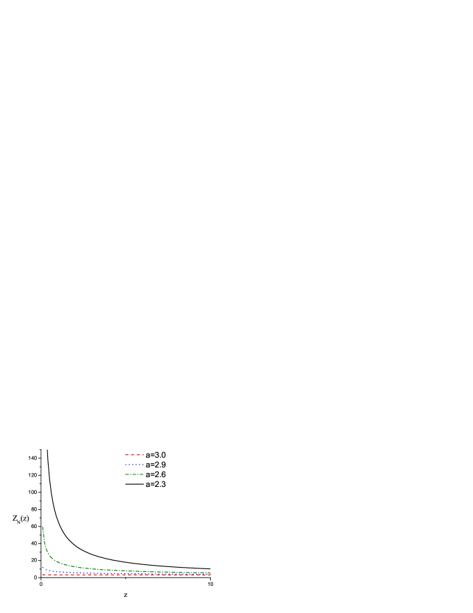
Figure 1: The partition function $Z_{N}(z)$ just at the adsorption thereshold $c=0$ and for $N=100$, as a function of $z/l$ for $1\ll z/l\ll N^{\nu}$ and for different values of $a$. $Z_{N}(z)$ is dimensionless and $l$ is the microscopic length scale.

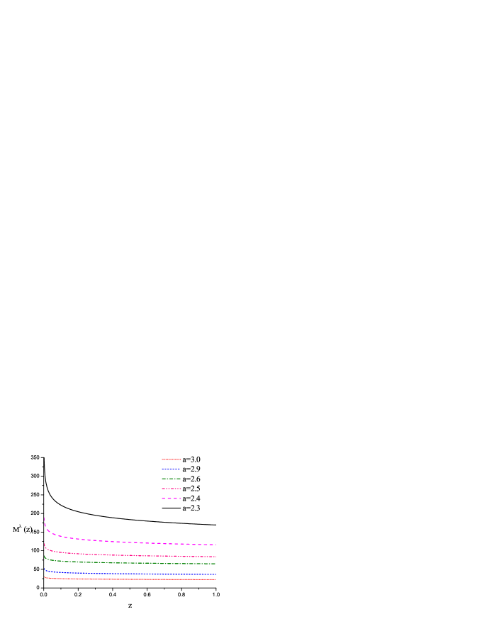
Figure 2: The density of monomers $M^{\lambda}(z)$ in the layer at the distance $z$ from the surface to which one end of the chain is attached for $1\ll z/l\ll N^{\nu}$ just at the threshold $c=0$ and for $N=100$ for different values of $a$. $M^{\lambda}(z)$ is in arbitrary units and $z/l$ is dimensionless.

Let us describe the effect of the long-range correlated disorder at the adsorption threshold and at the crossover to the adsorbed state assuming that the qualitative trends are properly captured by the one-loop results. For small distances ($l\ll z\ll\xi_{R}$) and for $c=0$ the partition function $Z_{N}(z)$ and the number of monomers in the layer at $z$ are shown in Figs. 1 and 2 respectively for several values of $a$. From these plots (see also Eqs. (10) and (11) and Tables I, II and Table in Ref.Blavatska01 ) we can see that the number of free ends and the number of monomers in the near-surface region ($l\ll z\ll\xi_{R}$) both increase for deceasing $a$. Moreover, the dependence on $z$ is the stronger, the larger the range of correlations between the defects. This result suggests that the larger is the range of correlations between the defects, the more efficient is the trapping of the chain between the attractive surface and the region occupied by the defects. For smaller $a$ more steps are necessary for the chain to go around the defected region, which is larger for smaller $a$. From the fact that $\Phi$ decreases for decreasing $a$ it follows that the fraction of the monomers adsorbed at the surface also decreases (see Eq.(9) and Table II). This result is somewhat surprising, since it shows a trend just opposite to the one for the fraction of monomers contained in the layer at the distance $z$ from the wall for $l\ll z\ll\xi_{R}$. A possible explanation might be that once the polymer leaves the surface, the large disordered patches in the bulk make it difficult for the polymer to return back. As a result, the fraction of the monomers near the wall can be higher than right at the wall. Recall that also in the pure systems for $c=0$ there is a discrepancy between the behavior of the fraction of monomers right at the surface, $N_{1}/N\sim N^{\Phi-1}$, and the fraction of monomers at the distance from the surface of the order of the effective monomer dimension $l$, $M^{\lambda}_{N}(l)/N\sim N^{\Phi-1+\gamma_{1}-1}$. Since $\gamma_{1}>1$ beyond MF, the concentration of monomers close to the surface is larger than just at the boundary, and $N_{1}/M^{\lambda}_{N}(l)\sim N^{1-\gamma_{1}}\to 0$ for $N\to\infty$ and $c=0$. Our one-loop results indicate that this effect is enhanced in the presence of long-range correlated disorder.

Let us now consider the crossover to the adsorbed state. Assume that one end of the infinite polymer chain is attached to the surface, and the temperature is decreased below the threshold, i.e. $-1<c<0$. The thickness of the adsorbed layer (Eq.(4)) starts to decrease from infinity when $|c|$ increases from zero (see Fig.3). From Eq.(2) and Table II we see that for a given $c$ such that $|c|<1$, the thickness of the near-surface, polymer layer increases when the range of correlations increases ($a$ decreases). Moreover, the dependence on $a$ of the exponent $\nu(a)/\Phi(a)$ is stronger than in the case of $\nu(a)$. Hence, the dependence of the thickness of the adsorbed layer $\xi\sim|c|^{-\nu(a)/\Phi(a)}$ on $a$ is stronger than the corresponding dependence of the mean end-to-end distance $\xi_{R}\sim N^{\nu(a)}$ in the bulk. It indicates that the effect of the long-range disorder on the adsorbed layer just below the threshold is stronger than the corresponding effect on the polymer coil in the bulk. The fraction of monomers, on the other hand, decreases for a fixed temperature for decreasing $a$, because for decreasing $a$, $\Phi(a)$ decreases (see Eq. (9) and Table II).

In Fig.4 the dependence of the fraction of monomers on the thickness of the adsorbed layer just below the threshold is shown for two values of $a$. Note that for a given value of the fraction of monomers at the surface the thickness of the adsorbed layer increases for decreasing $a$. Let us compare two systems, characterized by different ranges of disorder-correlations, $a_{1}<a_{2}$. Each system contains a chain with $N$ monomers. Assume finally that the same number of monomers $N_{1}$ is adsorbed at the surface in each system (of course temperatures in these systems are different, see (9) and Table II). The number of monomers inside the solution, $N-N_{1}$ is the same in the two considered cases. Since $a_{1}<a_{2}$, larger correlated patches have to be avoided by the chain in the first system. By analogy with the polymer properties in the bulk Blavatska01 it is natural to expect that the same number of monomers contained in the solution, $N-N_{1}$, must effectively occupy larger space in the case where larger correlated patches have to be surrounded by the chain. Our results are thus consistent with the former results for the bulk systems Blavatska01 .

We conclude that the long-range correlated disorder has a significant effect on the adsorption of polymers on the surface at and near the adsorption threshold. When one end of the polymer is attached to the surface, the perpendicular part of the average distance to the other end increases for increasing range of correlations between the disorder. At the same time, the fraction of monomers at the surface decreases for fixed temperature both at and below the threshold. Moreover, just at the threshold the monomer concentration near the wall (i.e. for $l\ll z\ll\xi_{R}$) increases. We should stress that the above conclusions follow from the results obtained in the one-loop approximation, and the possibility that the real dependence of the surface critical exponents on $a$ is different cannot be excluded. Two-loop calculations and/or computer simulations, going beyond the scope of this work, might help to draw definite conclusions.

Table 1: Surface critical exponents of the long-flexible polymer at the special transition $c=c_{a}$ for $d=3$ up to one-loop order calculated at the pure (the case $a=3$ with $(v^{*}=1.632,w^{*}=0)$) and LR stable fixed point for different fixed values of the correlation parameter, $2<a<3$.

$a$	$v^{*}$	$w^{*}$	$\eta_{\parallel}$		$\eta_{\perp}$		$\beta_{1}$		$\gamma_{11}$	$\gamma_{1}$
			$[1/0]$	$[0/1]$	$[1/0]$	$[0/1]$	$[1/0]$	$[0/1]$	$[1/0]$	$[1/0]$
3.0	1.63	0.00	-0.204	-0.169	-0.102	-0.114	0.250	0.250	0.704	1.255
2.9	4.13	1.47	-0.342	-0.255	-0.171	-0.146	0.247	0.248	0.837	1.418
2.8	4.73	1.68	-0.402	-0.287	-0.200	-0.167	0.244	0.244	0.891	1.480
2.7	5.31	1.81	-0.468	-0.319	-0.233	-0.189	0.241	0.241	0.951	1.550
2.6	5.89	1.87	-0.542	-0.351	-0.270	-0.212	0.238	0.238	1.018	1.630
2.5	6.48	1.89	-0.620	-0.383	-0.308	-0.236	0.235	0.236	1.090	1.715
2.4	7.10	1.87	-0.704	-0.413	-0.350	-0.259	0.233	0.233	1.169	1.810
2.3	7.76	1.84	-0.793	-0.442	-0.394	-0.283	0.230	0.231	1.253	1.911

Table 2: Surface critical exponents of the long-flexible polymer at the special transition $c=c_{a}$ for $d=3$ involving the RG function $\eta_{\bar{c}}$, calculated at the pure (the case $a=3$) and LR stable fixed point for different fixed values of the correlation parameter, $2<a<3$.

$a$	$v^{*}$	$w^{*}$	$\eta_{\bar{c}}$		$\alpha_{1}$		$\alpha_{\parallel}$		$\Phi$		$(1-\Phi)$	$/\nu$
			$[1/0]$	$[0/1]$	$[1/0]$	$[0/1]$	$[1/0]$	$[0/1]$	$[1/0]$	$[0/1]$	$[1/0]$	$[0/1]$
3.0	1.63	0.00	-0.362	-0.266	0.217	0.280	-0.362	-0.266	0.421	0.427	0.954	0.956
2.9	4.13	1.47	-0.607	-0.378	0.031	0.181	-0.607	-0.378	0.363	0.379	0.942	0.945
2.8	4.73	1.68	-0.710	-0.415	-0.045	0.147	-0.710	-0.415	0.335	0.358	0.950	0.953
2.7	5.31	1.81	-0.822	-0.451	-0.128	0.114	-0.822	-0.451	0.306	0.337	0.955	0.957
2.6	5.89	1.87	-0.943	-0.485	-0.219	0.082	-0.943	-0.485	0.276	0.317	0.954	0.956
2.5	6.48	1.89	-1.066	-0.516	-0.314	0.051	-1.066	-0.516	0.247	0.298	0.944	0.947
2.4	7.10	1.87	-1.192	-0.544	-0.413	0.023	-1.192	-0.544	0.222	0.282	0.922	0.928
2.3	7.76	1.84	-1.309	-0.567	-0.511	-0.003	-1.309	-0.567	0.203	0.271	0.881	0.894

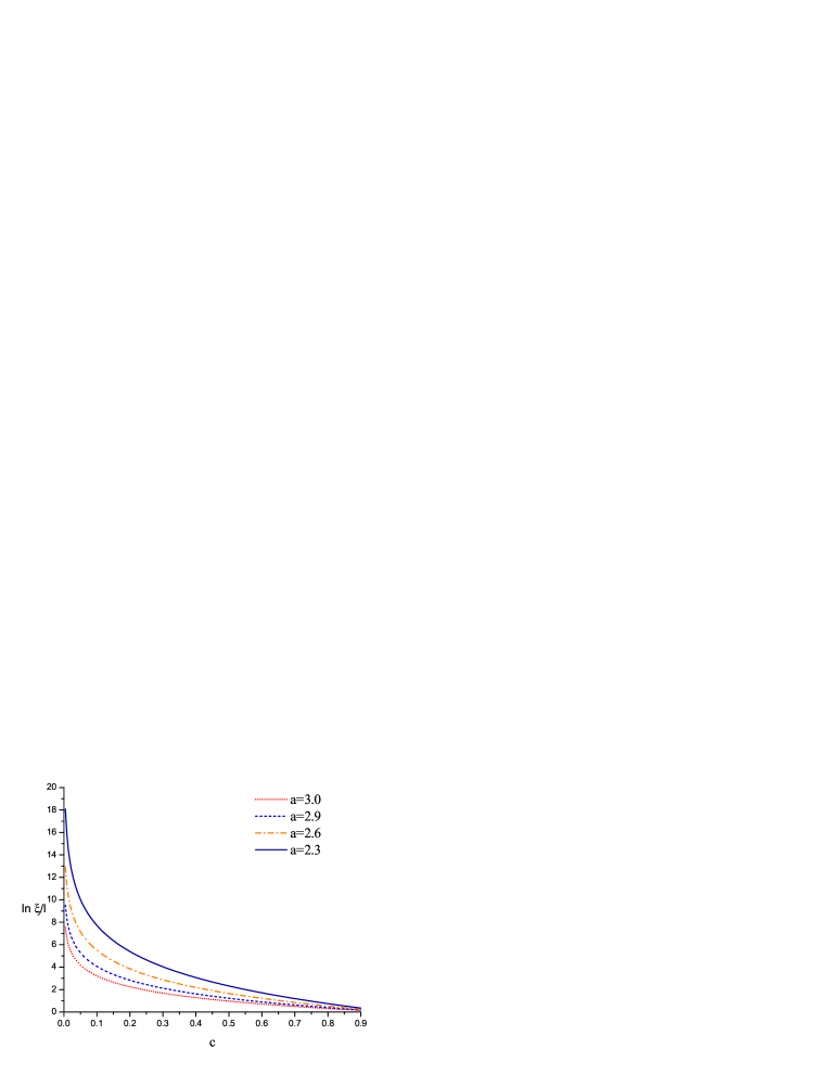
Figure 3: The dependence of the thickness of the adsorbed layer $\xi/l$ on $|c|$, for $c<0$, where $c\propto(T-T_{a})/T_{a}$ is the reduced temperature distance from the threshold, for different values of $a$. Both quantities are dimensionless.

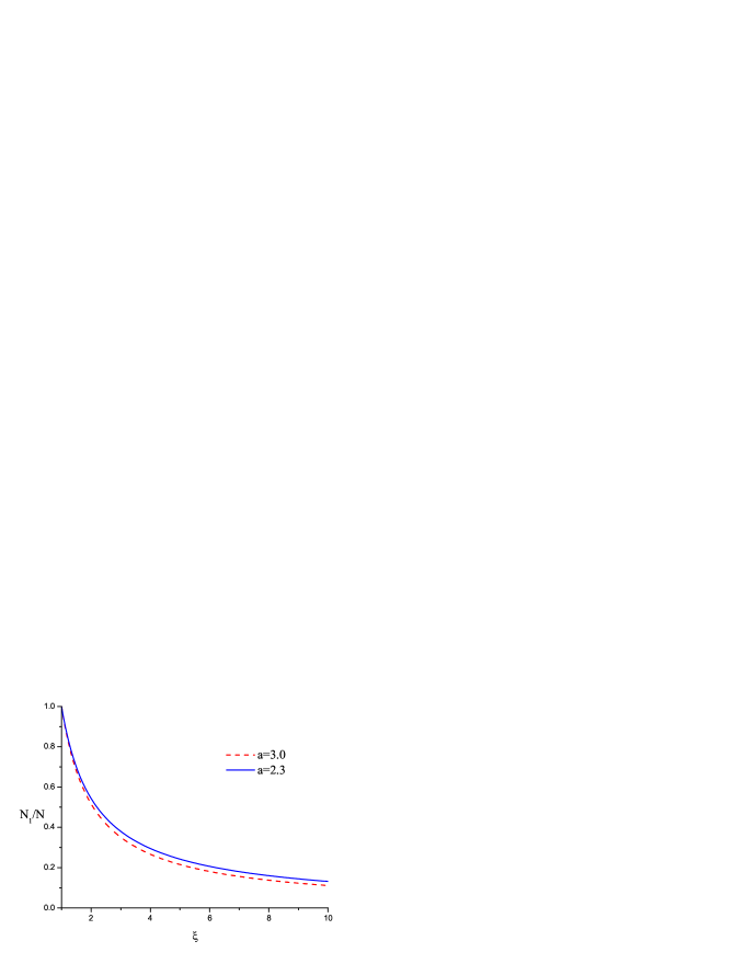
Figure 4: The dependence of the fraction of monomers at the surface $N_{1}/N$ on the thickness of the adsorbed layer $\xi/l$ for $c<0$ (i.e. below the threshold) and for two values of $a$, $a=3.0$ and $a=2.3$. Both quantities are dimensionless.

Appendix

The individual RG series expansions for the other critical exponents can be derived through standard surface scaling relations D86 with $d=3$

$$\eta_{\perp}=\frac{\eta+\eta_{\parallel}}{2},$$

$$\beta_{1}=\frac{\nu}{2}(d-2+\eta_{\parallel}),$$

$$\gamma_{11}=\nu(1-\eta_{\parallel}),$$

$$\gamma_{1}=\nu(2-\eta_{\perp}),$$ (A2.1)

$$\Delta_{1}=\frac{\nu}{2}(d-\eta_{\parallel}),$$

$$\delta_{1}=\frac{\Delta}{\beta_{1}}=\frac{d+2-\eta}{d-2+\eta_{\parallel}},$$

$$\delta_{11}=\frac{\Delta_{1}}{\beta_{1}}=\frac{d-\eta_{\parallel}}{d-2+\eta_{\parallel}}\;.$$

Each of these critical exponents characterizes certain properties of the semi-infinite systems with long-range quenched disorder, in the vicinity of the critical point. The values $\nu$, $\eta$, and $\Delta=\nu(d+2-\eta)/2$ are the standard bulk exponents.

References

• (1) V.Blavats’ka, C.von Feber, and Yu.Holovatch, J.Mol.Liq. 92, 77 (2001).
• (2) V.Blavats’ka,C.von Feber, Yu.Holovatch, Phys.Rev.E, 64, 041102 (2001).
• (3) P.-G. de Gennes, Scaling Concepts in Polymer Physics (Cornell University) Press, Ithaca, NY, 1979).
• (4) E.Eisenriegler, K. Kremer, and K. Binder, J. Chem. Phys. 77, 12 (1982).
• (5) E.Eisenriegler, J.Chem.Phys. 79, 1052 (1983)
• (6) E.Eisenriegler, Polymers near surfaces, World Scientific Publishing Co.Pte.Ltd., 1993.
• (7) R.Hegger and p.Grassberger, J.Phys.A 27, 4069 (1994).
• (8) Y.Singh, S.Kumar, and D.Giri, J.Phys.A 32, L407 (1999).
• (9) Y.Singh, D.Giri, and S.Kumar, J.Phys.A 34, L67 (2001).
• (10) R.Rajesh, D.Dhar, D.Giri, S.Kumar, and Y.Singh, Phys.Rev.E 65, 056124 (2002).
• (11) D.Zhao and T.Lookman, K.De’Bell, Phys.Rev.A 42, 4591 (1990).
• (12) H.W.Diehl and S.Dietrich, Z.Phys.B 42, 65 (1981).
• (13) H.W.Diehl and S.Dietrich, Z.Phys.B 50, 117 (1983).
• (14) H.Β W. Diehl, in Phase Transitions and Critical Phenomena, edited by C. Domb and J.Β L. Lebowitz (Academic Press, London, 1986), Vol.Β 10, pp.Β 75–267.
• (15) H. W. Diehl and A. NΓΌsser, Z. Phys. B 79, 69 (1990).
• (16) J.des Cloizeaux and G.Jannink, Polymers in Solution (Clarendon Press, Oxford, 1990); L.SchΓ€fer L, Universal Properties of Polymer Solutions as Explained by the Renormalization Group (Springer, Berlin, 1999).
• (17) P.G.de Gennes, J.Phys. (Paris) 37, 1445 (1976); M.Daoud and P.G. de Gennes, ibid. 38, 85 (1977).
• (18) M.N.Barber, A.S.Guttman, K.M.Middlemiss, G.M.Torrie, and S.G.Whittington, J.Phys.A 11, 1833 (1978).
• (19) H.Β W. Diehl and M. Shpot, Nucl. Phys. B 528, 595 (1998).
• (20) Y.Kim, J.Phys.C 16, 1345 (1983).
• (21) A. B. Harris, Z. Phys. B: Condens.Matter 49, 347 (1983).
• (22) A.Β B. Harris, Journ. Phys. C 7, 1671 (1974).
• (23) R.Guida and J.Zinn Justin J.Phys.A 31, 8104 (1998).
• (24) M. Shpot, Cond. Mat. Phys. N 10, 143 (1997).
• (25) Z.Usatenko, Chin-Kun Hu, Phys.Rev.E 65, 056102 (2001).
• (26) V.V.Prudnikov, P.V.Prudnikov, and A.A.Fedorenko, J.Phys.A 32, L399 (1999); V.V.Prudnikov, P.V.Prudnikov, and A.A.Fedorenko, ibid. 32,8587 (1999); V.V.Prudnikov, P.V.Prudnikov, and A.A.Fedorenko, Phys.Rev.B 62, 8777 (2000).
• (27) J.Zinn-Justin, Euclidean Field Theory and Critical Phenomena (Oxford Univ. Press, New York, 1989).
• (28) C.Bagnuls and C.Bervillier, Phys.Rev.B 24, 1226 (1981).
• (29) A.Ciach and U.Ritschel, Nucl.Phys.B 489, 653 (1997).
• (30) A. Weinrib and B. I. Halperin, Phys. Rev. B 27, 413 (1983).