Collapse of a Bose-Einstein condensate induced by fluctuations of the laser intensity

Abstract

The dynamics of a metastable attractive Bose-Einstein condensate trapped by a system of laser beams is analyzed in the presence of small fluctuations of the laser intensity. It is shown that the condensate will eventually collapse. The expected collapse time is inversely proportional to the integrated covariance of the time autocorrelation function of the laser intensity and it decays logarithmically with the number of atoms. Numerical simulations of the stochastic 3D Gross-Pitaevskii equation confirms analytical predictions for small and moderate values of mean field interaction.

I Introduction

The experimental realization of Bose-Einstein condensation (BEC) in dilute atomic gases davis95 ; anderson96 ; bradley97 founded a rapidly progressing new field of research dalfovo . The physical properties of BECs, which to date comprise eight elements Rb, Na, Li, H, He, K, Cs, Yb and their isotopes, are predominantly determined by interatomic forces. Some of the atomic species (⁷Li, ⁸⁵Rb, ¹³³Cs) possess a negative $s$-wave scattering length in the ground state and display attractive interactions. The attractive interaction between the atoms causes the collapse of the BEC so that a stable BEC was not believed to exist nozieres . However, when an external spatial confinement is imposed for instance by a system of laser beams, a trapping potential shows up which can counterbalance the attractive interaction and allows the formation of a metastable BEC. When the number of atoms increases, the attractive interaction becomes stronger and the energy barrier that prevents the 3D BEC from collapsing becomes weaker. To a given trapping potential there corresponds a critical number of atoms above which the energy barrier vanishes. The case of a quadratic potential has been studied, the critical number of atoms has been computed by a variational approach and by extensive numerical simulations of the Gross-Pitaevskii (GP) equation, and the results have been checked experimentally dalfovo ; roberts01 ; savage03 .

One of the most important aspects of BECs in the regime of attractive interactions is that they are unstable against collapse. The collapse shows up as a rapid and strong shrinking of the condensate at some critical number of atoms, and is accompanied by significant atomic losses due to many-body processes donley . The collapse is initiated when the balance of forces governing the size and shape of the condensate is altered either by internal or external factors. With respect to spatial and energetic stability the magnetic traps appear to be better controllable compared to optical traps grimm . On the other hand, due to increasing interest in far-off resonant laser traps for Bose-condensation of atoms which are insensitive to magnetic fields takasu , the investigation of different aspects of BEC dynamics in optical traps is becoming a very relevant subject. Of particular interest is the effect of temporal fluctuations of the laser intensity which in turn involve temporal fluctuations of the parabolic trapping potential savard . In the present paper we shall consider the BEC dynamics under random fluctuations of the strength of the parabolic trap potential and we shall show that small fluctuations can lead to the eventual collapse of the 3D BEC due to a cumulative effect of stochastic perturbations. The random fluctuations have all harmonics in their spectrum, and some of them participate in the parametric resonance leading to collapse. This stochastic parametric resonance in the BEC width oscillations has a rough equivalent particle picture: the Kramers’ exit problem which is concerned with noise activated escape from a potential well hanggi .

Quantum tunneling (QT) is considered as playing a key role in the condensate collapse when the number of atoms is close to the critical number leggett . We shall see that the BEC instability driven by random fluctuations of the strength of the parabolic trap potential is all the more dramatic as the number of atoms is closer to the critical number. Our consideration thus shows that even weak noise can play a competitive role in this limit with QT and should be taken into account. The effect of optical trap noise was previously considered in the context of stochastic heating of trapped atoms savard ; gehm . In a far-off resonant optical trap created by a system of red detuned lasers the variable trapping potential can be represented as $V(t,r)=-\alpha|E(t,r)|^{2}/4$, where $\alpha$ is the atomic polarizability and $E(t,r)$ is the electric field amplitude. The dynamics of trapped atoms can be described by the corresponding Hamiltonian $H=p^{2}/(2m)+(1/2)m\omega_{0}^{2}(1+\eta(t))r^{2}$, where $\omega_{0}^{2}=k_{0}^{2}/m$ is the mean square trap oscillation frequency, and $k_{0}$ is proportional to the time-averaged laser intensity $I_{0}\sim|E|^{2}$. The time dependent spring constant is determined by fractional fluctuations of the laser intensity $\eta(t)=(I(t)-I_{0})/I_{0}$ savard . The influence of the fluctuations of the trap potential on the dynamics of 1D GP type equation has been considered in ABP and the trap and nonlinearity fluctuations in two dimensional BEC in ABK ; ABG .

The paper is organized as follows. In Section II we give a description of the model and apply a variational approach. In Section III we derive the effective dynamics of the action-angle variables of the system driven by random perturbations. Section IV (resp. V) are devoted to the asymptotic analysis of the system for small (resp. near-critical) number of atoms. Finally we check the variational approach and our asymptotic analysis in Section VI by performing direct numerical simulations of the GP equation.

II The model and the variational approach

We consider the mean-field GP equation for the single-particle wave function gross

$$i\hbar\psi_{t}=-\frac{\hbar^{2}}{2m}\Delta\psi+V(t,{\bf r})\psi+g|\psi|^{2}\psi.$$ (1)

The nonlinear coefficient is $g=4\pi\hbar^{2}a_{s}/m$ where $a_{s}$ and $m$ are respectively the atomic scattering length and mass. The number of atoms is $N=\int|\psi|^{2}dx$. $V$ is the external trapping potential imposed by a system of laser beams. We consider a harmonic model, but we take into account temporal fluctuations of the laser intensity which in turn induces temporal fluctuations of the quadratic potential

$$V(t,{\bf r})=\frac{m\omega_{0}^{2}}{2}|{\bf r}|^{2}[1+\eta(t)].$$ (2)

For the optical trap $\omega^{2}=\alpha I/(2ml_{0}^{2})$, where $l_{0}$ is the size of the laser beam, $I$ is the intensity, $\alpha$ is a constant proportional to the laser frequency detuning. The random function $\eta(t)$ describes the laser intensity fluctuations $\eta(t)=(I(t)-I_{0})/I_{0}$. The stationary random process $\eta$ has zero-mean and standard deviation $\sigma_{\eta}$. We shall see in the following that the standard deviation is not sufficient to predict the collapse of the BEC, but the coherence time and more generally the power spectral density of $\eta$ will play a role.

We now cast Eq. (1) in a dimensionless form by introducing the variables $t^{\prime}=\omega_{0}t$, ${\bf r}^{\prime}={\bf r}/r_{0}$, $r_{0}^{-1}=\sqrt{m\omega_{0}/\hbar}$, and $u=\sqrt{4\pi|a_{s}|r_{0}^{2}}\psi$. This yields the following partial differential equation (PDE)

$$iu_{t^{\prime}}=-\frac{1}{2}\Delta^{\prime}u+\frac{1}{2}|{\bf r}^{\prime}|^{2}[1+\eta^{\prime}(t^{\prime})]u+\sigma_{s}|u|^{2}u,$$ (3)

where $\sigma_{s}={\rm sgn}(a_{s})=\pm 1$ and $\eta^{\prime}(t^{\prime})=\eta(t^{\prime}/\omega_{0})$. From now on we drop the primes. The next step consists in applying the variational approach. This approximation was first introduced by Anderson anderson83 and developed in nonlinear optics malomed . A similar technique was elaborated for the BEC dynamics based on the GP equation perez97 . The variational ansatz for the wave function of the BEC is chosen as the Gaussian dalfovo

$$u(t,{\bf r})=A(t)\exp\left(-\frac{|{\bf r}|^{2}}{2a(t)^{2}}+\frac{ib(t)|{\bf r}|^{2}}{2}+i\theta(t)\right).$$ (4)

$a(0)r_{0}$ is the initial BEC rms width in physical variables

$$a(0)=\frac{\sqrt{2}}{\sqrt{3}\sqrt{N}r_{0}}\left(\int|{\bf r}|^{2}|\psi(t=0,{\bf r})|^{2}d^{3}{\bf r}\right)^{1/2}.$$

The number of atoms is

$$N=\frac{\sqrt{\pi}r_{0}}{4|a_{s}|}A(0)^{2}a(0)^{3}=\frac{\sqrt{\pi}r_{0}}{4|a_{s}|}A(t)^{2}a(t)^{3}.$$

Following the standard procedure malomed , we substitute the ansatz into the Lagrangian density generating Eq.(3) and calculate the effective Lagrangian density in terms of $A$, $a$, $b$, $\theta$ and their time-derivatives. The evolution equations for the parameters of the ansatz are then derived from the effective Lagrangian by using the corresponding Euler-Lagrange equations. In particular this approach yields a closed-form ordinary differential equation (ODE) for the BEC width $a$

$$a_{tt}+a(1+\eta(t))=\frac{1}{a^{3}}+\frac{\sigma_{s}P}{a^{4}},$$ (5)

where $P=\sqrt{2/\pi}N|a_{s}|/r_{0}$. We study in this paper the attractive case ($a_{s}<0$, $\sigma_{s}=-1$). The evolution equation finally reads

$$a_{tt}+a(1+\eta(t))=\frac{1}{a^{3}}-\frac{P}{a^{4}}.$$ (6)

III Action-angle variables

III.1 Unperturbed dynamics

The energy $E$ of the unperturbed BEC is given by:

$$E(t)=\frac{1}{2}a_{t}^{2}(t)+{U}(a(t)),\hskip 7.22743pt{U}(a)=\frac{1}{2}\left(a^{2}+\frac{1}{a^{2}}\right)-\frac{P}{3a^{3}}.$$ (7)

In absence of random fluctuations $\eta\equiv 0$ the energy $E$ is an integral of motion. The BEC width obeys a simple dynamics with Hamiltonian structure

$$H(p,q)=\frac{1}{2}p^{2}+{U}(q)$$ (8)

with $q=a$ and $p=a_{t}$. A straightforward analysis ruprecht ; dalfovo shows that if $P<P_{c}=4/5^{5/4}\simeq 0.535$, then the potential $U$ possesses a local minimum that we shall denote by $a_{0}$ (see Fig. 1). The corresponding ground state has energy $E_{0}=U(a_{0})$. Below $a_{0}$ there is the local maximum $a_{1}$ with energy $E_{1}=U(a_{1})$, and below $a_{1}$ the potential decays to $-\infty$. Above $a_{0}$ the potential increases to $+\infty$. It crosses the energy level $E_{1}$ at $a_{2}$.

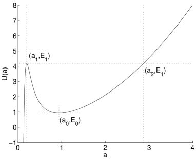
Figure 1: Potential $U(a)$ for $P=0.2$. The important points $(a_{1}<a_{0}<a_{2})$ are also represented.

If the initial conditions $(a(0),a_{t}(0))$ correspond to an energy above $E_{1}$, or below $E_{1}$ but $a(0)<a_{1}$, then the condensate width goes to zero in finite time which means that the BEC collapses. On the contrary, if the initial conditions $(a(0),a_{t}(0))$ correspond to an energy between $E_{0}$ and $E_{1}$, and $a(0)>a_{1}$, then the orbits of the motion are closed, corresponding to periodic oscillations. In order to explicit the periodic structure of the variables $a$ and $a_{t}$, we introduce the action-angle variables. The orbits are determined by the energy imposed by the initial conditions:

$$E=\frac{1}{2}a_{t}^{2}(0)+{U}(a(0)).$$

For $E\in(E_{0},E_{1})$, we introduce $e_{1}(E)<e_{2}(E)$ the extremities of the orbit of $a$ for the energy $E$:

$$U(e_{1}(E))=U(e_{2}(E))=E.$$

The action $I$ is defined as a function of the energy $E$ by

$${\cal I}(E)=\frac{1}{2\pi}\oint pdq=\frac{1}{\pi}\int_{e_{1}(E)}^{e_{2}(E)}\sqrt{2E-2{U}(b)}db.$$ (9)

The motion described by (8) is periodic, with period

$${\cal T}(E)=\oint\frac{dq}{p}=2\int_{e_{1}(E)}^{e_{2}(E)}\frac{db}{\sqrt{2E-2{U}(b)}}$$ (10)

or else ${\cal T}(E)=2\pi\frac{d{\cal I}}{dE}(E)$. The angle $\phi$ is defined as a function of $I$ and $a$ by

$$\phi(E,a)=-\int^{a}\frac{\partial p}{\partial I}dq=-\frac{2\pi}{{\cal T}(E)}\int^{a}\frac{db}{\sqrt{2E-2{U}(b)}}.$$

The transformation $(E,a)\rightarrow(I,\phi)$ can be inverted to give the functions ${\cal E}(I)$ and ${\cal A}(I,\phi)$. The BEC width oscillates between the minimum value $e_{1}(E)$ and the maximum value $e_{2}(E)$. The energy $E$ as well as the action $I$ are constant and fixed by the initial conditions, so the evolution of the BEC width is governed by

$$a(t)={\cal A}({\cal I}(E),\phi(t)),$$

$$\phi(t)=\phi(0)-\frac{2\pi}{{\cal T}(E)}t.$$

III.2 Perturbed dynamics

From now on we assume $\eta\not\equiv 0$ and we denote by $\sigma_{\eta}$ the standard deviation of $\eta$. We investigate the stability of the BEC when the unperturbed motion is oscillatory. In particular we aim at studying the collapse time $T_{c}$ defined as the first time $t$ such that $a(t)=0$. While the energy of the BEC is below $E_{1}$, the orbit is closed. As soon as the energy reaches the energy level $E_{1}$, the BEC collapses in a time of order $1$ (w.r.t. $\sigma_{\eta}$). We shall show that the hitting time for the energy level $E_{1}$ is of order $\sigma_{\eta}^{-2}$, so the collapse time $T_{c}$ is imposed by the hitting time $T_{h}$ defined as the first time $t$ such that $E(t)=E_{1}$ or equivalently $I(t)=I_{1}:={\cal I}(E_{1})$.

In presence of perturbations, the motion of $a$ is not purely oscillatory, because the energy and the action are slowly varying in time. We adopt the action-angle formalism, because it allows us to separate the fast scale of the locally periodic motion and the slow scale of the evolution of the action. Thus, after rescaling $\tau=\sigma_{\eta}^{2}t$ the action-angle variables satisfy the differential equations

$$\left\{\begin{array}[]{l}\displaystyle\frac{dI}{d\tau}=\frac{1}{\sigma_{\eta}}\eta(\frac{\tau}{\sigma_{\eta}^{2}})h_{\phi}(I,\phi),\\ \displaystyle\frac{d\phi}{d\tau}=-\frac{1}{\sigma_{\eta}^{2}}\omega(I)-\frac{1}{\sigma_{\eta}}\eta(\frac{\tau}{\sigma_{\eta}^{2}})h_{I}(I,\phi),\end{array}\right.$$ (11)

where $h(I,\phi)=\frac{1}{2}{\cal A}^{2}(I,\phi)$ and $\omega(I)=\frac{2\pi}{{\cal T}({\cal E}(I))}$ are smooth functions and $h$ is periodic with respect to $\phi$ with period $2\pi$. The normalization $\tau=\sigma_{\eta}^{2}t$ has been chosen so that the random process $\eta$ appears with the scales of a white noise in the differential equations (11). Applying a standard diffusion-approximation theorem psv , we get that $(I(t))_{t\geq 0}$ behaves like a diffusion Markov process with the infinitesimal generator

$${\cal L}_{{I}}=\frac{1}{2}A({I})\frac{\partial^{2}}{\partial{I}^{2}}+B({I})\frac{\partial}{\partial{I}}$$

where

$$A({I})=\frac{1}{\pi}\int_{0}^{2\pi}\int_{0}^{\infty}h_{\phi}({I},\phi)h_{\phi}({I},\phi-\omega({I})t){\mathbb{E}}[\eta(0)\eta(t)]dtd\phi,$$

$$B({I})=\frac{1}{\pi}\int_{0}^{2\pi}\int_{0}^{\infty}h_{\phi}({I},\phi)h_{\phi I}({I},\phi-\omega({I})t){\mathbb{E}}[\eta(0)\eta(t)]dtd\phi.$$

This means in particular that the probability density function of ${I}(t)$ satisfies the Fokker-Planck equation $\partial_{t}p={\cal L}_{I}^{*}p$, $p(t=0,{I})=\delta({I}-I_{0})$, where $I_{0}$ is the initial action at time $0$ and ${\cal L}_{I}^{*}$ is the adjoint operator of ${\cal L}_{I}$, i.e. ${\cal L}_{I}^{*}p=(1/2)\partial_{I}^{2}\left[A({I})p\right]-\partial_{I}\left[B({I})p\right]$. Moreover, standard results of stochastic analysis allow us to compute recursively the moments of $T_{h}$ feller . Denoting $I_{1}={\cal I}(E_{1})$, the first moment ${\cal\mu}^{(1)}(I)={\mathbb{E}}_{I}[T_{h}]$ (the mean value of $T_{h}$ starting from action $I$ at time $0$) satisfies

$${\cal L}_{I}\mu^{(1)}=-1,\ \ \ \ \mu^{(1)}(I_{1})=0.$$ (12)

The $n$-th moment ${\cal\mu}^{(n)}(I)={\mathbb{E}}_{I}[T_{h}^{n}]$ satisfies

$${\cal L}_{I}\mu^{(n)}=-n\mu^{(n-1)},\ \ \ \ \mu^{(n)}(I_{1})=0.$$ (13)

In the following sections we shall apply and discuss these general results in two different frameworks: small and critical nonlinearity.

IV Small nonlinearity

IV.1 Expansions of the action-angle variables for small nonlinearity

In this section we assume that $P\ll 1$ which will allow us to derive simple expressions for the physically relevant quantities. The points $a_{j}$ and $E_{j}$ can be expanded for small nonlinearity $P$ as

$$a_{0}=1+O(P),\ \ \ \ a_{1}=P+O(P^{2}),\ \ \ \ a_{2}=\frac{1}{\sqrt{3}P}+O(1),$$

$$E_{0}=1+O(P),\ \ \ \ E_{1}=\frac{1}{6P^{2}}+O(\frac{1}{P}).$$

Note that, as $P$ becomes small, the potential barrier grows like $P^{-2}$, which shows that the trap looks like a deep quadratic external potential. The functions $h(I,\phi)$ and $\omega(I)$ can also be expanded for any $\phi$ and $I\leq I_{1}={\cal I}(E_{1})=1/(12P^{2})+O(1/P)$:

$$h(I,\phi)=\frac{1}{2}+I+\sqrt{I+I^{2}}\cos(\phi)+O(P),$$

$$\omega(I)=2+O(P).$$

Accordingly the unperturbed dynamics of the BEC width for small $P$ is approximately

$$a(t)=\sqrt{1+2I_{0}+2\sqrt{I_{0}+I_{0}^{2}}\cos(2t)}.$$ (14)

Figure 2 shows that this approximation is indeed very good for the orbit $a(t)$ whatever the initial conditions lying in a closed orbit with energy $<E_{1}$.

(a)

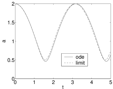
(b)

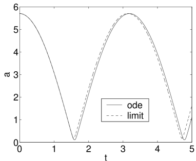
Figure 2: Unperturbed dynamics of the BEC width. We assume $P=0.1$, $a_{t}(0)=0$, $a(0)=2$ (picture a), $a(0)=5.7$ (picture b). The second case corresponds to an energy very close to $E_{1}$. The results from the resolution of the ODE are compared with the asymptotic formula (14).

IV.2 Effective equations in presence of perturbations

In case of small nonlinearity $P\ll 1$, the above expansions allow us to derive simple effective equations for the BEC action in presence of perturbations. Applying the general results obtained in Section III.2, we get that the action $I(t)$ behaves like a diffusion process with the infinitesimal generator

$${\cal L}_{{I}}=\frac{1}{2}\alpha_{c}\frac{\partial}{\partial{{I}}}\left[({{I}}+{{I}}^{2})\frac{\partial}{\partial{{I}}}\right]$$

where

$$\alpha_{c}=\int_{0}^{\infty}\cos(2t){\mathbb{E}}[\eta(0)\eta(t)]dt.$$

The expression of ${\cal L}_{{I}}$ holds true only for ${I}<I_{1}$. We can compute the growths of the first moments of the action starting from the ground state $I=0$ while $e^{\alpha_{c}t}\ll P^{-2}$:

$${\mathbb{E}}_{0}[{I}(t)]=\frac{1}{2}e^{\alpha_{c}t}-\frac{1}{2},$$ (15)

$${\mathbb{E}}_{0}[{I}(t)^{2}]=\frac{1}{6}e^{3\alpha_{c}t}-\frac{1}{2}e^{\alpha_{c}t}+\frac{1}{3}.$$ (16)

An empirical way to estimate the mean disintegration time is to look for the time $t_{1}$ such that ${\mathbb{E}}_{0}[I(t_{1})]=I_{1}$, where $I_{1}=1/(12P^{2})$. From Eq. (15) we get $t_{1}=(1/\alpha_{c})\ln[1+1/(6P^{2})]$. This argument is rough because the expectations are ill-placed. The exact results provided by the rigorous stochastic analysis confirm that this prediction is not correct. Integrating Eqs. (12-13) we get that the expectation of the disintegration time starting from the ground state $I=0$ is

$${\mathbb{E}}_{0}[T_{h}] = \frac{2}{\alpha_{c}}\ln(1+\frac{1}{12P^{2}})$$

$$\stackrel{{\scriptstyle P\ll 1}}{{\simeq}} \frac{2}{\alpha_{c}}\left(-2\ln(P)-\ln(12)\right),$$

while its variance is

$${\rm Var}_{0}(T_{h}) = \frac{8}{\alpha_{c}^{2}}\left[\ln(1+\frac{1}{12P^{2}})+{\rm dilog}(1+\frac{1}{12P^{2}})+\frac{1}{2}\ln(1+\frac{1}{12P^{2}})^{2}\right]$$

$$\stackrel{{\scriptstyle P\ll 1}}{{\simeq}} \frac{8}{\alpha_{c}^{2}}\left[-2\ln(P)-\ln(12)-\frac{\pi^{2}}{6}\right],$$

where the dilogarithm function is the tabulated function defined as follows:

$${\rm dilog}(x)=\int_{1}^{x}\frac{\ln(y)}{1-y}dy.$$

Equations (IV.2-IV.2) are the most important results of this paper. They show that the collapse time varies as $\sim\ln(P^{-2})$, while the energy barrier is $\sim P^{-2}$. In physical variables, the expected collapse time is

$${\mathbb{E}}_{0}[T_{c}]=\frac{2}{\omega_{0}\alpha}\ln\left(1+\frac{\hbar\pi}{24m\omega_{0}a_{s}^{2}N^{2}}\right),\ \ \ \ \alpha=\omega_{0}\int_{0}^{\infty}\cos(2\omega_{0}t){\mathbb{E}}[\eta(0)\eta(t)]dt.$$

Taking the experimental data $\omega_{0}=10$kHz, $N\simeq 5\cdot 10^{3}$, $a_{s}=-5$nm, and $\alpha=10^{-4}-10^{-5}$, we obtain the expected collapse time $\approx(1-10)$ seconds.

IV.3 Numerical simulations

We compare the theoretical predictions with numerical simulations of the ODE (6). We use a fourth-order Runge-Kutta method for the resolution of the ODE. The random fluctuations are modeled by a stepwise constant random process:

$$\eta(t)=\sigma\sum_{j}X_{j}{\bf 1}_{[jt_{c},(j+1)t_{c})}(t),$$

where the $X_{j}$ are independent and identically distributed random variables with uniform distribution over $(-{1}/2,{1}/2)$ and $t_{c}$ is the coherence time of the laser. The coefficient $\alpha_{c}$ is then given by

$$\alpha_{c}=\sigma^{2}\frac{1-\cos(2t_{c})}{48t_{c}};$$

The first series of simulations were performed with the parameters $\sigma=0.3$ and $t_{c}=0.5$. We investigate different configurations corresponding to different values of the parameter $P$ starting from $a(0)=1$, $a_{t}(0)=0$ which is very close to the ground state. We have carried $1000$ simulations for each configuration. The theoretical values for the expected value and standard deviation according to formulas (IV.2-IV.2) are reported in Table 1 and compared with the values obtained from averaging of the results of the numerical simulations.

Table 1: Comparisons between the averages and rms of the collapse time obtained from numerical simulations and from theoretical formulas. Here $\sigma=0.3$ and $t_{c}=0.5$.

	$\left<\tau\right>$			${\rm rms}(\tau)$
$P$	num	theor	error	num	theor	error
$0.05$	$4112$	$4103$	$0.2\%$	$2241$	$2335$	$4\%$
$0.1$	$2585$	$2591$	$0.2\%$	$1718$	$1601$	$7\%$
$0.2$	$1257$	$1306$	$3.5\%$	$833$	$865$	$4\%$
$0.3$	$586$	$760$	$23\%$	$407$	$518$	$21\%$
$0.4$	$205$	$486$	$58\%$	$165$	$336$	$51\%$

Note that the statistical formulas are theoretically valid in the asymptotic framework $P\ll 1$. The numerical simulations show that they are actually valid for $P\leq 0.2$. More exactly, the comparisons between the theoretical predictions and the numerical simulations shows excellent agreement for the mean values, and very good agreement also for the standard deviations. We also plot in Fig. 3 the histograms of the collapse times for two series of simulations.

(a)

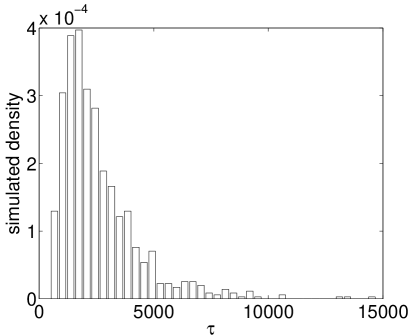
(b)

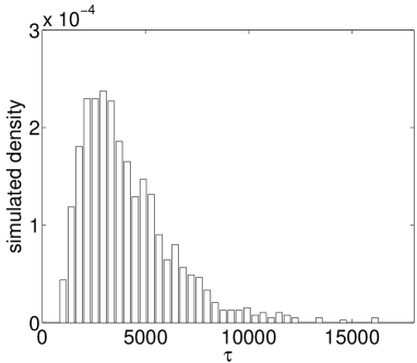
Figure 3: Histograms of the collapse time obtained from series of $1000$ simulations. Picture a: $P=0.1$. Picture b: $P=0.05$.

Table 2: Comparisons between the averages and rms of the collapse time obtained from numerical simulations and from theoretical formulas. Here $\sigma=2$ and $t_{c}=0.5$.

	$\left<\tau\right>$			${\rm rms}(\tau)$
$P$	num	theor	error	num	theor	error
$0.05$	$98.6$	$92.3$	$6.4\%$	$55.5$	$52.5$	$5.4\%$
$0.1$	$63.7$	$58$	$8.5\%$	$39.1$	$36.0$	$7.9\%$
$0.2$	$31.9$	$29.4$	$7.8\%$	$21.2$	$19.5$	$8.2\%$
$0.3$	$16.1$	$17.1$	$6.5\%$	$11.4$	$11.7$	$2.6\%$
$0.4$	$6.6$	$10.9$	$65\%$	$4.9$	$7.6$	$55\%$

Finally, in Table 2, we report results with a high level of fluctuations (namely $\sigma=2$). The theoretical predictions are still in agreement with the numerical simulations for $P\leq 0.3$ with an accuracy of $10\%$ although the considered configurations are at the boundary of the validity of the asymptotic theory.

V Critical nonlinearity

V.1 Expansions of the action-angle variables for critical nonlinearity

In this section we address the case where the nonlinear parameter $P$ is close to the critical value $P_{c}=4/5^{5/4}$. We do so by setting $P=P_{c}-\delta$ and assuming $\delta\ll 1$. Once again, all quantities can be expanded in powers of $\delta$. After some algebra, we get

$$a_{j}=a_{g}+2^{-1/2}5^{-1/8}\tilde{a}_{j}\delta^{1/2}+O(\delta)\mbox{ with }a_{g}=5^{-1/4},\ \ \ \tilde{a}_{0}=1,\ \ \ \tilde{a}_{1}=-1,\ \ \ \tilde{a}_{2}=2,$$

$$E_{j}=E_{g}+2^{1/2}3^{-1}5^{7/8}\tilde{E}_{j}\delta^{3/2}+O(\delta^{2})\mbox{ with }E_{g}=3^{-1}5^{1/2}+3^{-1}5^{3/4}\delta,\ \ \ \tilde{E}_{0}=-1,\ \ \ \tilde{E}_{1}=1.$$

More generally, if $a\in[a_{1},a_{2}]$, then it can be parameterized as $a=a_{g}+2^{-1/2}5^{-1/8}\delta^{1/2}\tilde{a}$ and the potential at $a$ can be expanded as

$$U(a)=E_{g}+2^{1/2}3^{-1}5^{7/8}\delta^{3/2}\tilde{U}(\tilde{a})+O(\delta^{2}),$$

where

$$\tilde{U}(\tilde{a})=\frac{1}{2}(\tilde{a}^{3}-3\tilde{a}).$$

Note that locally (i.e. around $a_{g}$) the potential presents a local minimum at $a_{0}$ (see Figure 4a), but the shape of the potential well is very different from the one observed in the framework $P\ll 1$ (compare with Fig. 1). The width of the well $a_{2}-a_{1}$ is of the order $\sqrt{\delta}$ and its depth $E_{1}-E_{0}$ is of order $\delta^{3/2}$. The local shape of the potential is given by the cubic function $\tilde{U}$.

(a)

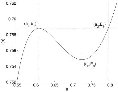
(b)

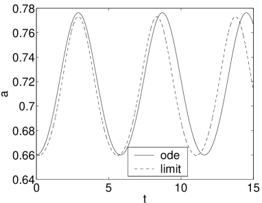
Figure 4: Picture a: Potential $U(a)$ for $P=P_{c}-0.01\simeq 0.525$ ($\delta=0.01$). Picture b: Unperturbed dynamics of the BEC width. We assume $a_{t}(0)=0$, $a(0)=0.66$, $\delta=0.01$. The results from the resolution of the ODE are compared with the asymptotic formula (20).

We now consider the action-angle variables. If $E\in[E_{1},E_{2})$, then it can be parameterized as $E=E_{g}+2^{1/2}3^{-1}5^{7/8}\tilde{E}\delta^{3/2}$ with $\tilde{E}\in[\tilde{E}_{0},\tilde{E}_{1})$. There exist three solutions $e_{3}(\tilde{E})\leq\tilde{a}_{1}\leq e_{1}(\tilde{E})\leq e_{2}(\tilde{E})\leq\tilde{a}_{2}$ of the cubic equation $\tilde{U}(\tilde{a})=\tilde{E}$. $e_{1}(\tilde{E})$ and $e_{2}(\tilde{E})$ determine the extremities of the orbit of the normalized width $\tilde{a}$ for the normalized energy $\tilde{E}$ in case of unperturbed dynamics. The cubic equation can be solved:

$$e_{j}(\tilde{E})=2\cos\left(\frac{{\rm arccos}(\tilde{E})+2\pi(j-2)}{3}\right).$$

In particular, if $E=E_{0}$ (i.e. $\tilde{E}=\tilde{E}_{0}$), then $e_{1}(\tilde{E}_{0})=e_{2}(\tilde{E}_{0})=1$ (and $e_{3}(\tilde{E}_{0})=-2$), which corresponds to the ground state $a(t)\equiv a_{0}$, or $\tilde{a}(t)\equiv 1$.

The period ${\cal T}(E)$ of the closed orbit at energy level $E$, as defined by (10), can be expanded as well. Introducing

$$\tilde{\cal T}(\tilde{E})=\delta^{1/4}2^{-1/4}5^{9/16}{\cal T}(E_{g}+2^{1/2}3^{-1}5^{7/8}\tilde{E}\delta^{3/2}),$$

we get that $\tilde{\cal T}$ is at leading order with respect to $\delta$ a $O(1)$-function that can be expressed in terms of tabulated functions

$$\tilde{\cal T}(\tilde{E})=\frac{2\sqrt{3}}{\sqrt{e_{2}(\tilde{E})-e_{3}(\tilde{E})}}K\left(\rho(\tilde{E})\right),$$

where

$$\rho(\tilde{E})=\frac{e_{2}(\tilde{E})-e_{1}(\tilde{E})}{e_{2}(\tilde{E})-e_{3}(\tilde{E})}$$

and $K$ is the complete elliptic integral (abra, , p. 590). We then define a normalized action $\tilde{\cal I}(\tilde{E})$ for $\tilde{E}\in[\tilde{E}_{0},\tilde{E}_{1}]=[-1,1]$ by

$$\tilde{\cal I}(\tilde{E})=\frac{1}{2\pi}\int_{-1}^{\tilde{E}}\tilde{\cal T}(s)ds.$$

The function $\tilde{\cal I}:[\tilde{E}_{0},\tilde{E}_{1}]\rightarrow[0,\tilde{I}_{1}]$ is invertible. Its inverse is denoted by $\tilde{\cal E}:[0,\tilde{I}_{1}]\rightarrow[\tilde{E}_{0},\tilde{E}_{1}]$ where $\tilde{I}_{1}=18/(5\pi)$. It is plotted in Fig. 5a. We can see that $\tilde{\cal E}$ is roughly linear. Similarly we can define the angle ${\cal\phi}(\tilde{E},\tilde{a})$ and its inverse $\tilde{\cal A}(\tilde{I},\phi)$. The function $\tilde{\cal A}:[0,\tilde{I}_{1}]\times[0,2\pi)\rightarrow[\tilde{a}_{1},\tilde{a}_{2}]$ can be expressed in terms of Jacobian elliptic functions

$$\tilde{\cal A}(\tilde{I},\phi)={e}_{1}(\tilde{\cal E}(\tilde{I}))+\left[{e}_{2}(\tilde{\cal E}(\tilde{I}))-{e}_{1}(\tilde{\cal E}(\tilde{I}))\right]{\rm sn}^{2}\left(\frac{K(\rho(\tilde{\cal E}(\tilde{I}))}{\pi}\phi,\rho(\tilde{\cal E}(\tilde{I}))\right),$$ (19)

where sn is the Jacobian sinus (abra, , p. 589). In absence of perturbation the action is preserved and the closed orbit of $\tilde{a}(t)$ for a normalized action $\tilde{I}\in[0,\tilde{I}_{1})$ is given by

$$\tilde{a}(t)=\tilde{\cal A}\left(\tilde{I},\phi(t)\right)\ \mbox{ with }\ \phi(t)=-\delta^{1/4}2^{-1/4}3^{-1/2}5^{9/16}\frac{2\pi}{\tilde{\cal T}(\tilde{\cal E}(\tilde{I}))}.$$ (20)

The true orbit is $a(t)=a_{g}+2^{-1/2}5^{-1/8}\delta^{1/2}\tilde{a}(t)$. Figure 4b shows that this approximation (derived in the asymptotic framework $\delta\ll 1$) is indeed reasonably good.

V.2 Effective equations in presence of perturbations

Following the strategy presented in Section III.2, we introduce the normalized action-angle variables so that $\tilde{E}(t)=\tilde{\cal E}(\tilde{I}(t))$ and $\tilde{a}(t)=\tilde{\cal A}(\tilde{I}(t),\phi(t))$. While the energy of the BEC is below $E_{1}$, the orbit is closed. As soon as the energy reaches the energy level $E_{1}$, the BEC collapses in a time of order $1$ (w.r.t. $\sigma_{\eta}$). We shall show that the hitting time for the energy level $E_{1}$ is of order $\sigma_{\eta}^{-2}$, so the collapse time $T_{c}$ is imposed by the hitting time $T_{h}$ defined as the first time $t$ such that $\tilde{I}(t)=\tilde{I}_{1}$. Here we rescale $\tau=\sigma_{\eta}^{2}\delta^{-3/2}t$. This normalization is chosen so that the random process $\eta$ appears with the scales of a white noise in the differential equations

$$\left\{\begin{array}[]{l}\displaystyle\frac{d\tilde{I}}{d\tau}=\frac{1}{\varepsilon}\eta(\frac{\tau}{\varepsilon^{2}})\tilde{h}_{\phi}(\tilde{I},\phi),\\ \displaystyle\frac{d\phi}{d\tau}=-\frac{\delta^{1/4}}{\varepsilon^{2}}2^{-1/4}5^{9/16}\tilde{\omega}(I)-\frac{1}{\varepsilon}\eta(\frac{\tau}{\varepsilon^{2}})\tilde{h}_{\tilde{I}}(\tilde{I},\phi),\end{array}\right.$$

where $\varepsilon=\sigma_{\eta}\delta^{-3/4}$, $\tilde{h}(\tilde{I},\phi)=2^{-5/4}3\ 5^{-11/16}\tilde{\cal A}(\tilde{I},\phi)$, and $\tilde{\omega}(\tilde{I})=\frac{2\pi}{\tilde{\cal T}(\tilde{\cal E}(\tilde{I}))}$. Note once again that $\tilde{h}$ and $\tilde{\omega}$ are smooth functions, and $\tilde{h}$ is periodic with respect to $\phi$ with period $2\pi$. By applying a diffusion approximation theorem psv , we get that $(\tilde{I}(t))_{t\geq 0}$ behaves like a diffusion Markov process with the infinitesimal generator

$${\cal L}_{\tilde{I}}=\alpha\delta^{-3/2}\frac{\partial}{\partial\tilde{I}}\tilde{A}(\tilde{I})\frac{\partial}{\partial\tilde{I}}$$

where

$$\tilde{A}(\tilde{I}) = 2^{-1/2}3^{2}5^{-11/8}\left[\tilde{e}_{2}(\tilde{\cal E}(\tilde{I}))-\tilde{e}_{1}(\tilde{\cal E}(\tilde{I}))\right]^{2}\frac{K(\rho(\tilde{\cal E}(\tilde{I}))}{\pi^{2}}\int_{0}^{K(\rho(\tilde{\cal E}(\tilde{I}))}{\rm cn}^{2}{\rm dn}^{2}{\rm sn}^{2}\left(s,\rho(\tilde{\cal E}(\tilde{I}))\right)ds,$$

$$\alpha = \int_{0}^{\infty}{\mathbb{E}}[\eta(0)\eta(t)]dt,$$

and dn and cn are two tabulated elliptic functions (abra, , p. 589). The conditions ensuring the diffusion-approximation are $\delta\ll 1$, $\sigma_{\eta}^{2}\ll\delta^{3/2}$. The diffusion coefficient $\tilde{A}(\tilde{I})$ is plotted in Fig. 5b.

(a)

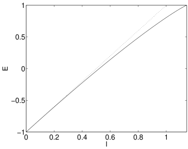
(b)

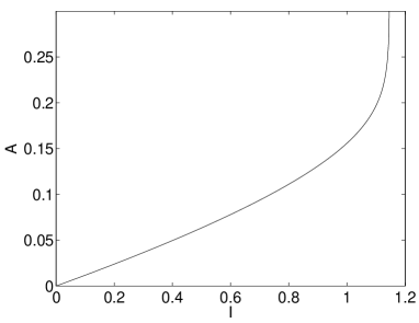
Figure 5: Functions $\tilde{I}\mapsto\tilde{\cal E}(\tilde{I})$ (picture a) and $\tilde{I}\mapsto\tilde{A}(\tilde{I})$ (picture b).

Using the results reported in Section III.2 we get the following recursive relation ($n\geq 1$) for the moments of the hitting time $T_{h}$

$${\mathbb{E}}_{\tilde{I}}[T_{h}^{n}]=\frac{n\delta^{3/2}}{\alpha}\int_{\tilde{I}}^{\tilde{I}_{1}}\frac{\int_{0}^{x}{\mathbb{E}}_{y}[T_{h}^{n-1}]dy}{\tilde{A}(x)}dx,$$ (21)

where $\tilde{I}_{1}=18/(5\pi)$. In dimensional variables, the result reads as follows. Starting from the ground state $a_{0}$, the expected value of the collapse time is

$${\mathbb{E}}_{0}[T_{c}]=\frac{\left(P_{c}-P\right)^{3/2}}{\omega_{0}^{2}\alpha}C_{1},$$ (22)

where $C_{1}$ is the constant $C_{1}=\int_{0}^{\tilde{I}_{1}}\frac{x}{\tilde{A}(x)}dx$. By a numerical integration using Matlab we have found $C_{1}\simeq 8.5$. More generally, we have

$${\mathbb{E}}_{0}[T_{c}^{n}]=\frac{\left(P_{c}-P\right)^{3n/2}}{\omega_{0}^{2n}\alpha^{n}}C_{n},$$ (23)

where $C_{n}$ are constants obtained recursively from Eq. (21). By a numerical integration we have found $C_{2}\simeq 110$.

V.3 Numerical simulations

We compare the theoretical predictions with numerical simulations of the ODE (6). We use the same model as in Section IV.3 with the parameters $\sigma=0.025$ and $t_{c}=0.5$. We report in Table 3 the theoretical values for the expected value and standard deviation according to formulas (22-23) as well as the values obtained from averaging of the results of the numerical simulations. The statistical formulas are theoretically valid in the asymptotic framework $\delta(=P_{c}-P)\ll 1$. The numerical simulations show that they are actually valid for $\delta\leq 0.03$.

Table 3: Comparisons between the averages and rms of the collapse time obtained from numerical simulations and from theoretical formulas.

		$\left<\tau\right>$			${\rm rms}(\tau)$
$P$	$\delta$	num	theor	error	num	theor	error
$0.525$	$0.01$	$651$	$653$	$0.3\%$	$447$	$472$	$5\%$
$0.515$	$0.02$	$1754$	$1846$	$5\%$	$1240$	$1334$	$7.5\%$
$0.505$	$0.03$	$3175$	$3392$	$7\%$	$2217$	$2451$	$10.5\%$
$0.495$	$0.04$	$4673$	$5222$	$11.5\%$	$3107$	$3775$	$21.5\%$

VI Validation of the variational approach

The analysis carried out in this paper is based on the variational approach using a Gaussian ansatz. The Gaussian ansatz for the study of static and dynamic properties of trapped gases has been widely used (see for instance perez97 ; shi97 ; stoof97 ; parola98 ; abdullaev01 ). The variational principle is shown in these papers to be a simple Lagrangian-based method that gives reasonable accurate ordinary differential equations approximations to the true dynamics for the solution of the GP equation. This method merely assumes Gaussian pulse shapes containing a fixed number of free parameters and the Lagrangian form of the partial differential equation is used to obtain the parameter evolution equations. However it is a questionable approach because it is based on the a priori assumption that the solution of the PDE has a form which remains very close to the chosen ansatz. Accordingly it has to be checked carefully by full numerical simulations of the PDE.

Numerical simulations of the stochastic GP equation with spherically symmetric trap is performed by Crank-Nicholson scheme. The absorbing boundary condition is employed to imitate the infinite domain size. This technique allows to prevent re-entering of linear waves emitted by the condensate under perturbation into the integration domain. We have first checked the variational approach for the unperturbed system. We have done so by inserting the Gaussian waveform with the amplitude and width corresponding to a stationary point (as predicted by the variational approach) as an initial condition into the PDE (3). We have let the solution evolve in time and we have plotted the results in Fig. 6a. As can be seen the Gaussian ansatz is a good approximation when $P$ is not close to the critical value $P_{c}$. Actually we have found numerically that the critical value for the existence of the BEC is not $P_{c}=0.535$, as predicted by variational approximation, but $P_{c}=0.459$. For $P$ very close to the real value of $P_{c}$, the Gaussian ansatz substantially deviates from the exact solution of the 3D GP equation, as shown in Fig. 6b.

In a second step we have performed numerical simulations of the GP equation (3) driven by a random Gaussian white noise $\eta$ with zero-mean and autocorrelation function ${\mathbb{E}}[\eta(t)\eta(t^{\prime})]=\sigma^{2}\delta(t-t^{\prime})$. We do so by choosing randomly and independently the value of $\eta$ at each time step. The mean collapse time is calculated as an average over 100 realizations of random paths along which the width of the condensate evolves from the value corresponding to the minimum of the effective potential $a_{0}$ until the value corresponding to its local maximum $a_{1}$ (see Fig. 1). The initial wave-form is selected as a Gaussian with parameters predicted by the variational approximation corresponding to the stationary state of the condensate. Fig. 7a represents the collapse time for different values of the parameter $P$ which are not too close to the critical value $P_{c}$. Comparison with the results from numerical simulations of the ODE (5) shows a very good agreement. This demonstrates that the variational approach provides accurate predictions for the behavior of the BEC. for small non-linearity, and that the asymptotic analysis carried out in Section IV holds true for the randomly driven GP equation.

(a)

(b)

Figure 6: Picture a: Width of the BEC for an initial Gaussian waveform with parameters corresponding to a stationary point of the potential $U(a)$. The oscillations are insignificant for small values of $P$, and become important when $P$ approaches the critical value $P_{c}=0.459$. At overcritical $P$ the waveform rapidly shrinks ($a\rightarrow 0$), i.e. the BEC undergoes collapse. Picture b: Exact solution of the 3D GP equation (solid line) compared with the Gaussian approximation with the same number of atoms and $P=0.44$.

(a)

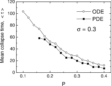
(b)

Figure 7: Mean collapse time calculated from stochastic PDE simulations (solid squares) and compared with the corresponding stochastic ODE simulations (open circles). Each mean is computed by averaging over a series of $100$ simulations. Picture a: Mean collapse time as a function of $P$ for a white noise strength $\sigma=0.3$. Picture b: Mean collapse time as a function of $\sigma$ for a nonlinear parameter $P=0.44$ close to the critical value $P_{c}=0.459$.

Finally, we have performed numerical simulations of the GP equation (3) driven by a white noise $\eta$ with a nonlinear parameter $P$ very close to the critical value $P_{c}=0.459$. For near-critical values of the parameter $P$ the Gaussian waveform was found to be not enough accurate. In this case we employed the exact solution of the GP equation to initiate random simulations. The exact solution (ground state) of the GP equation is found by imaginary time-evolution method as described in chiofalo . It is plotted in Fig. 6b. The results are plotted in Fig. 7b. We can see that collapse in the perturbed PDE occurs much earlier than in the ODE model. This shows that the BEC in full GP equation is unstable against collapse at near critical nonlinear parameter. A small perturbation can drive the BEC to collapse through fluctuations that are not captured by the variational approach. Accordingly, we can state that the variational approach provides poor predictions for the behavior of the BEC for critical non-linearity. Several reasons can explain the departure: 1) the Gaussian ansatz is not correct (see Fig. 6b). 2) the study of the ODE model shows that the important parameter in the near-critical case is not the value of $P$, but the value of the difference between $P$ and $P_{c}$. But the ODE does not capture the correct value of $P_{c}$, so the error committed in the evaluation of the difference $P-P_{c}$ becomes very large when $P$ becomes close to $P_{c}$. 3) radiation effects become very important, in the sense that the waveform is strongly affected, even when the simulations are performed starting from the exact numerical waveform plotted in Fig. 6b, so that we feel that it is useless to try to find a more suitable ansatz. In this respect, one should add that this result is not surprising because it is well known in nonlinear optics that the time-dependent variational approach fails to describe the regime near the collapse kuznetsov ; berge . Finally, it is necessary to mention that the behavior of the gas close to collapse can be affected by mechanisms that are not included in the GP equation, such as inelastic two and three-body collisions edwards96 ; fedichev96 .

VII Conclusion

We have considered in this paper a condensate trapped by an external potential generated by a system of laser beams in the case of a negative scattering length. We have studied the stability of the metastable BEC against small fluctuations of the laser intensity. We have shown that collapse of the BEC occurs whatever the amplitude of the fluctuations after a time which is inversely proportional to the integrated covariance of the autocorrelation function of the fluctuations of the laser intensity. The statistical distribution of the collapse time has been computed. The dependence of the mean collapse time with respect to the number atoms $N$ has been thoroughly analyzed. We have shown that, for $N$ below the critical number of atoms $N_{c}$, the mean collapse time decreases logarithmically with increasing $N$. As a byproduct of the analysis we have shown that the variational approach is very efficient for the analysis of the BEC for a number of atoms $N$ which is not too close to $N_{c}$, but we have seen that it completely fails for $N$ close to $N_{c}$.

VIII Acknowledgments

F. Kh. A. and B. B. B. are grateful to the Fund of fundamental researches of the Uzbekistan Academy of Sciences for the partial financial support. B.B.B. also thanks the Physics Department of the University of Salerno, Italy, for a research grant.

References

- (1) K. B. Davis, M. O. Mewes, M. R. Andrews, N. J. van Druten, D. S. Durfee, D. M. Kurn, and W. Ketterle, Phys. Rev. Lett. 75, 3969 (1995).
- (2) M. H. Anderson, J. R. Ensher, M. R. Mathews, C. E. Wieman, and E. A. Cornell, Science 269, 198 (1995).
- (3) C. C. Bradley, C. A. Sackett, and R. G. Hulet, Phys. Rev. Lett. 78, 985 (1997).
- (4) F. Dalfovo, S. Giorgini, L. P. Pitaevskii, and S. Stringary, Rev. Mod. Phys. 71, 463 (1999).
- (5) P. Nozières and D. Pines, The theory of quantum liquids (Addison Wesley, Reading, 1990).
- (6) J. L. Roberts, N. R. Claussen, S. L. Cornish, E. A. Donley, E. A. Cornell, and C. E. Wieman, Phys. Rev. Lett. 86, 4211 (2001).
- (7) C. M. Savage, N. P. Robins, and J. J. Hope, Phys. Rev. A 67, 014304 (2003).
- (8) E. A. Donley, N. R. Claussen, S. L. Cornish, J. L. Roberts, E.A. Cornell, and C.E. Wieman, Nature, 412, 295, (2001).
- (9) R. Grimm, M. Weidemüller and Y. B. Ovchinnikov, Adv. At. Mol. Opt. Phys. 42, 95 (2000).
- (10) Y. Takasu, K. Maki, K. Komori, T. Takano, K. Honda, M. Kumakura, T. Yabuzaki, and Y. Takahashi, Phys. Rev. Lett. 91, 040404 (2003).
- (11) T. A. Savard, K. M. O’Hara, and J. E. Thomas, Phys. Rev. A 56 R1095, (1997).
- (12) P. Hänggi, P. Talkner, and M. Borkovec, Rev. Mod. Phys. 62, 251 (1990).
- (13) M. Ueda and A. J. Leggett, Phys. Rev. Lett. 80, 1576 (1998).
- (14) M. E. Gehm, K. M. O’Hara, T. A. Savard, and J. E. Thomas, Phys. Rev. A 58, 3914 (1998).
- (15) F. Kh. Abdullaev, J. C. Bronski, and G. Papanicolaou, Physica D 135, 369 (2000).
- (16) F. Kh. Abdullaev, B. B. Baizakov, and V. V. Konotop, In Nonlinearity and Disorder: Theory and Applications, NATO Science Series, Vol. 45, F. Kh. Abdullaev, O. Bang and M. P. Soerensen (Eds), (Kluwer, Dodrecht, 2001).
- (17) F. Kh. Abdullaev, J. C. Bronski, and R. Galimzyanov, arXive:cond-mat/0205464.
- (18) E. P. Gross, Nuovo Cimento 20, 454 (1961); J. Math. Phys. 4, 195 (1963); L. P. Pitaevskii, Zh. Eksp. Teor. Fiz. 40, 646 (1961) [Sov. Phys. JETP 13, 451 (1961)].
- (19) D. Anderson, Phys. Rev. A 27, 3135 (1983).
- (20) B.A. Malomed, Prog. Opt. 43, 69 (2002).
- (21) V.M. Pérez-García, H. Michinel, J.I. Cirac, M. Lewenstein, and P. Zoller, Phys. Rev. A 56, 1424 (1997).
- (22) P. A. Ruprecht, M. J. Holland, K. Burnett, and M. Edwards, Phys. Rev. A 51, 4704 (1995).
- (23) G. Papanicolaou and W. Kohler, Comm. Pure Appl. Math. 27, 641 (1974).
- (24) W. Feller, An introduction to probability theory and its applications (Wiley, New York, 1971).
- (25) M. Abramowitz and I. A. Stegun, Handbook of mathematical functions (Dover, New York, 1972).
- (26) H. Shi and W.-M. Zheng, Phys. Rev. A 55, 2930 (1997).
- (27) H. T. C. Stoof, J. Stat. Phys. 87, 1353 (1997).
- (28) A..Parola, L. Salasnich, and L. Reatto, Phys. Rev. A 57, R3180 (1998).
- (29) F. Kh. Abdullaev, A. Gammal, Lauro Tomio, and T. Frederico, Phys. Rev. A 63, 043604 (2001).
- (30) M. L. Chiofalo, S. Succi, and M. P. Tosi, Phys. Rev. E 62, 7438 (2000).
- (31) E. A. Kuznetsov, A. M. Rubenchik, and V. E. Zakharov, Phys. Rep. 142, 103 (1986).
- (32) L. Bergé, Phys. Rep. 303, 260 (1998).
- (33) M. Edwards, P. A. Ruprecht, K. Burnett, R. J. Dodd, and C. W. Clark, Phys. Rev. Lett. 77, 1671 (1996).
- (34) P. O. Fedichev, M. W. Reynolds, and G. V. Shlyapnikov, Phys. Rev. Lett. 77, 2921 (1996).