Failure of Scattering Interference in the Pseudogap State of Cuprate Superconductors

Abstract

We calculate scattering interference patterns for various electronic states proposed for the pseudogap regime of the cuprate superconductors. The scattering interference models all produce patterns whose wavelength changes as a function of energy, in contradiction to the energy-independent wavelength seen by scanning tunneling microscopy (STM) experiments in the pseudogap state. This suggests that the patterns seen in STM local density of states measurements are not due to scattering interference, but are rather the result of some form of ordering.

The origin of pseudogap phenomena is one of the key questions in the cuprate superconductors, as it profoundly affects their properties above the superconducting transition, and potentially influences the cuprate phase diagram. Timusk In a recent paper, we have used a scanning tunneling microscope to show that the electronic states in the pseudogap state of $Bi_{2}Sr_{2}CaCu_{2}O_{8+\delta}$ are spatially modulated. Vershinin These electronic modulations in the local density of states, which are seen only for energies less than the pseudogap energy scale, are oriented along the copper-oxide bond direction and have an energy-independent, incommensurate wavelength. One interpretation of these experiments is that these modulations are caused by electronic ordering, a variety of which have been proposed for the cuprates in the pseudogap regime. SachdevOrder ; Eduardo ; Demler ; Zhang ; DHLOrder Another possibility is that such modulations are the consequence of scattering interference from one of the electronic states proposed for the pseudogap. Franz ; Norman The interest in scattering interference as a possible explanation is motivated by the success of this idea in understanding similar modulations in the superconducting state Hoffman ; DHLee ; McElroy , although even below $T_{c}$ there are a number of deviations from the scattering interference picture. Eduardo ; Howald ; Vortex ; DavisOrder In this paper, we elaborate on calculations reported in Ref. 2 to demonstrate the failure of the scattering interference scenario in describing the modulations observed in the pseudogap state. We show that this failure is a generic feature of scattering interference itself, regardless of the model chosen for the pseudogap electronic state. Franz ; ArcFit ; Levin ; DDW ; MFL This shortcoming suggests that the modulations observed in the pseudogap regime are the signature of some form of ordering.

The scattering interference picture ascribes spatial modulations in the local density of states to interference between elastically scattered quasiparticles. Balatsky ; DHLee A well-studied example of this phenomenon is the standing wave patterns seen on certain metal surfaces, in which electrons scattering from step edges and point impurities interfere coherently to form modulations in the density of states. Eigler The period of these modulations at a given energy $\omega$ is determined by the wavevector $\vec{q}$ that joins the two points on curves of constant electron energy in $\vec{k}$ space with the greatest weight, as determined by the electronic structure of the system. For a superconductor, the scattering interference contribution to the local density of states can be treated within the Born approximation, which introduces a correction,

$$\delta n(\vec{r},\omega)=-{1\over\pi}Im\{\int{d^{2}\vec{r_{1}}G_{0}(\vec{r}-\vec{r_{1}},\omega)V(\vec{r_{1}},\omega)G_{0}(\vec{r_{1}}-\vec{r},\omega)-F_{0}(\vec{r}-\vec{r_{1}},\omega)V(\vec{r_{1}},\omega)F_{0}(\vec{r_{1}}-\vec{r},\omega)}\}$$ (1)

to the density of states, where $G_{0}$ and $F_{0}$ are the single particle and anamolous Green functions, respectively, and $V$ is a weak, finite-range scattering potential. Franz ; DHLee ; Capriotti ; Sachdev ; Yeh ; Hirschfeld For pure potential scattering, the Fourier transform of the Born correction $\delta n(\vec{q},\omega)=-{1\over\pi}Im\{V(\vec{q},\omega)\Lambda(\vec{q},\omega)\}$ seperates into a part

$$\Lambda(\vec{q},\omega)=\int\{d^{2}\vec{k}G_{0}(\vec{k},\omega)G_{0}(\vec{k}+\vec{q},\omega)-$$

$$F_{0}(\vec{k},\omega)F_{0}(\vec{k}+\vec{q},\omega)\}$$ (2)

which contains all the wave interference information, and a part

$$V(\vec{q},\omega)=\int{d^{2}\vec{x}e^{-i\vec{q}\cdot\vec{x}}V(\vec{x},\omega)}$$ (3)

which acts like a static structure factor. Capriotti For now, we will assume that the structure factor does not filter any wave interference information.

In order to develop a context in which to understand quantum interference in the pseudogap state, we will first review the quantum interference picture for the two cases already discussed in the literature- the superconducting state and the Fermi liquid normal state. DHLee ; Capriotti ; Sachdev ; Hirschfeld Following these previous works, scattering interference in the superconducting state can be modeled using the Green functions,

$$G_{0}(\vec{k},\omega)={\omega+i\delta+\epsilon_{\vec{k}}\over{(\omega+i\delta-\epsilon_{\vec{k}})(\omega+i\delta+\epsilon_{\vec{k}})-{\Delta_{\vec{k}}^{2}}}}$$

$$F_{0}(\vec{k},\omega)={\Delta_{\vec{k}}\over{(\omega+i\delta-\epsilon_{\vec{k}})(\omega+i\delta+\epsilon_{\vec{k}})-{\Delta_{\vec{k}}^{2}}}}$$ (4)

where $\epsilon_{\vec{k}}=120.5-595.1\times(\cos{k_{x}}+\cos{k_{y}})/2+163.6\times\cos{k_{x}}\cos{k_{y}}-51.9\times(\cos{2k_{x}}+\cos{2k_{y}})/2-111.7\times(\cos{2k_{x}}\cos{ky}+\cos{k_{x}}\cos{2k_{y}})/2+51.0\times(\cos{2k_{x}}\cos{2k_{y}})$ is the $Bi_{2}Sr_{2}CaCu_{2}O_{8+\delta}$ band structure from ARPES BS for slightly underdoped ($\delta=.12$) samples, $\Delta_{\vec{k}}=45.0\times(\cos{k_{x}}+\cos{k_{y}})/2$ is the superconducting gap function, and $\delta$ is a broadening term. As shown in Figures 1a and b, this yields pictures with sharp peaks in q-space which disperse. To understand the origin of the dispersion qualitatively, it helps to consider a simplified version of scattering interference, the so-called octet model, introduced by Hoffman et al. and McElroy et al.. Hoffman ; McElroy Quasiparticles can elastically scatter between points on contours of constant electron energy in k-space (Fig. 1c). The shape of these contours changes continuously as the energy increases. Consequently, the length of the characteristic scattering interference wavevector (q-space) changes, leading to dispersion. This picture changes dramatically if, instead of a superconducting Green function, we use a Fermi liquid normal state Green function by setting $\Delta_{\vec{k}}=0$ in Equation 4. Capriotti The sharp peaks in q-space for the superconducting state have been replaced with dispersing caustics (Figs. 1a and d). The equivalence of all points in k-space leads directly to an absence of sharp peaks in q-space. The dispersion is now a direct consequence of the band structure itself. Although the Fermi liquid scattering interference picture is useful in determining the effect of the band structure on scattering interference, it is not applicable to the pseudogap, as it omits two key features of this state: the pseudogap in the density of states, and the ill-defined nature of quasiparticles.

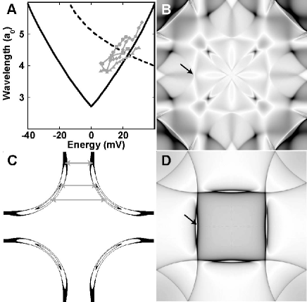
Figure 1: (A) STM data in the superconducting state shows modulations in the local density of states which disperse. Shown here is data taken along the $(0,\pi)$ direction (the Cu-O bond direction) from Vershinin et al. Vershinin at 40K for slightly underdoped $Bi_{2}Sr_{2}CaCu_{2}O_{8+\delta}$ (sqaures), and from Hoffman et al. Hoffman at 4K for underdoped (triangle), as-grown (diamond) and overdoped (circle) samples. The wavelength is in units of $a_{0}=3.8\AA$, the Cu-Cu distance. The solid black line shows the dispersion for the $(0,\pi)$ mode in the superconducting state calculated using Born scattering. The dashed black line shows the dispersion of the $(0,\pi)$ mode for the Fermi liquid normal state. (B) The power spectrum of $\delta n(\vec{q},\omega)$ in the superconducting state with a broadening of 1mV is shown here in the first Brillouin zone at an energy of $\omega=20mV$. Black regions correspond to a large contribution from scattering interference. The dispersion of the slowest dispersing feature along the $(0,\pi)$ direction, highlighted by the arrow, is plotted as the solid black line in (A). The $F_{0}$ term in Eq. 4 makes the $(\pi,\pi)$ mode have sharp peaks, but makes the $(0,\pi)$ mode weaker for non-magnetic impurities. The situation is reversed for the magnetic impurity case (not shown), in which the $F_{0}$ term has the opposite sign. Franz (C) The solid black lines show contours of constant electron energy in the superconducting state at $\omega=0mV$ (point along $(\pi,\pi)$ direction), $\omega=\Delta/2$ (small banana) and $\omega=\Delta$ (large banana). The most prominent peaks in scattering wavevector space (q-space) along the $(0,\pi)$ direction are indicated by the grey arrows. (D) The power spectrum of $\delta n(\vec{q},\omega)$ in the Fermi liquid normal state with a broadening of 1mV is shown here in the first Brillouin zone at an energy of $\omega=20mV$. The dispersion of the slowest dispersing feature along the $(0,\pi)$ direction, highlighted by the arrow, is plotted as the dashed black line in (A).

To extend the scattering interference model into the pseudogap regime, we must first choose an appropriate Green function with which to model the pseudogap state. Although its origin is still not understood, the pseudogap has been thoroughly characterized by ARPES in the underdoped cuprate superconductors. Arcs At all energies, peaks in the ARPES spectral function are so broad that it is unclear whether quasiparticles are still well-defined. SAG Meanwhile, at the Fermi energy, the spectral function shows extended arcs centered at the nodal points (Fig. 2a) in k-space. As energy increases towards the pseudogap energy scale, these arcs extend towards the Brilouin zone boundary. Theoretical attempts at understanding the measured behaviour have either followed a phenomenological approach, or have proposed exotic electronic states for the pseudogap. We will first focus on the phenomenological attempts. Norman et al. have modeled the ARPES data in the pseudogap regime using the Green function

$$G_{0}(\vec{k},\omega)=(\omega-\epsilon_{\vec{k}}-\Sigma_{\vec{k}})^{-1}$$ (5)

and $F_{0}=0$, where the self energy,

$$\Sigma(\vec{k},\omega)=-i\Gamma_{1}+\Delta_{\vec{k}}^{2}/(\omega+\epsilon_{\vec{k}}+i\Gamma_{0}),$$ (6)

$\Gamma_{1}$ is a single particle scattering rate, $\Gamma_{0}$ is a measure of decoherence, and $\Delta_{\vec{k}}$ is a gap function with a $\vec{k}$ dependence which matches the Fermi arcs. ArcFit The calculated scattering interference patterns (Fig. 2b) have two notable shortcomings in comparison with the measured data shown in Figure 2c. First, the calculated patterns contain caustics, while the measured patterns contain discrete points along the $(0,\pi)$ directions. This shortcoming can be overcome by assuming, for example, that the STM tunneling matrix element has a $d$-wave symmetry and selectively filters the density of states along the $(0,\pi)$ direction. Second, the scattering interference patterns calculated from this phenomenological description still show features along the $(0,\pi)$ directions that disperse (Fig. 2d). This dispersion curve resembles that in the superconducting state, as the characteristic wavevector for scattering interference is of a similar length at the gap energy, but is shallower because this wavevector is much shorter at the Fermi energy in the pseudogap regime (Figs. 1c and 2a). Even this shallower dispersion results in a change of wavelength between $7a_{0}$ and $4.6a_{0}$ between the Fermi energy and the pseudogap energy, whereas STM experiments show a fixed wavelength of $4.7\pm 0.2a_{0}$ over this energy range. Vershinin

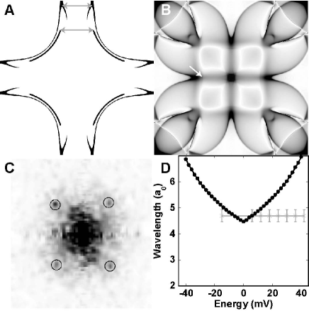
Figure 2: (A) Shown in black are model representations of the electronic density of states in k-space measured by ARPES at the Fermi energy (arcs centered at the nodal points) and at the pseudogap energy (banana). Shown in gray are the shortest wavevectors along the $(0,\pi)$ direction for scattering interference at the two respective energies. (B) We calculated the power spectrum of $\delta n(\vec{q},\omega)$ for a phenomenological Fermi arc Green function where the extent of the Fermi arcs were chosen to give a scattering wavelength of $4.6a_{0}$ at the Fermi energy, and unphysically small values of $\Gamma_{0}=1mV$ and $\Gamma_{1}=1mV$ were chosen to produce sharper features. The power spectrum of $\delta n(\vec{q},\omega)$ for this Fermi arc picture is shown here in the first Brillouin zone at $\omega=20mV$. The dispersion of the most slowly dispersing feature along the $(0,\pi)$ direction, indicated by the arrow, is shown in (D) as a solid line. (C) The power spectrum of the STM data at 15mV in the pseudogap state from Vershinin et al. Vershinin shows four peaks along the $(0,\pi)$ direction (circles). We have magnified the data to show only the relevant region in q-space. (D) These peaks in q-space correspond to a fixed wavelength of $4.7\pm 0.2a_{0}$, shown here as the grey line. Also shown is the dispersion of the most slowly dispersing feature along the $(0,\pi)$ direction in scattering interference calculations for the Fermi arc Green function. This feature disperses similar to the $(0,\pi)$ mode in the superconducting state for small ($\approx 1mV$) values of $\Gamma_{0}$ and $\Gamma_{1}$. Larger ($\approx 10mV$) values of $\Gamma_{0}$ lead to the gradual suppression of this mode in favor of a mode which disperses similar to the band structure (Fig. 1a). Larger values of $\Gamma_{1}$ yield pictures which average over some part of the dispersion for a particular mode, leading to unphysically broad features.

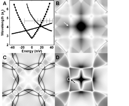
Figure 3: (A) The dispersions of all the exotic electronic state Green functions discussed in the text should be resolved by the STM experiment. Shown are the dispersions of the most slowly dispersing $(0,\pi)$ modes for the $QED_{3}$ (squares), DDW (up triangles) and circulating current (down triangles) Green functions. These modes are labeled by the arrows in parts (B), (C), and (D). STM data from the pseudogap state Vershinin is shown in gray. (B) The power spectrum of $\delta n(\vec{q},\omega)$ for a $QED_{3}$ Green function is shown here in the first Brillouin zone at $\omega=20mV$. The patterns were calculated using a value of $\eta=0.4$ and a broadening of 1mV. For increased $\eta$, the patterns in q-space become more diffuse until, by $\eta\approx 1$, there are no discernable features in q-space. (C) The power spectrum of $\delta n(\vec{q},\omega)$ for a DDW Green function using a broadening of 1mV and a chemical potential shift of $+40meV$ is shown here in the first Brillouin zone at $\omega=20mV$. (D) The power spectrum of $\delta n(\vec{q},\omega)$ for a circulating current Green function using $\lambda=.27$, $T=10mV$, $D_{0}=10mV$, and $\omega_{c}=500mV$ is shown here in the first Brillouin zone at $\omega=20mV$. Non-zero values of $D_{0}$ result in the slowest dispersing mode along the $(0,\pi)$ direction (arrow) being replaced by a faster dispersing mode (circle) at energies $\omega<|2\times D_{0}|$. The dispersion shown in part (A) is for $D_{0}=0$, corresponding to the slowest dispersing mode.

We next consider the scattering interference scenario for various exotic electronic states proposed for the pseudogap regime. We will discuss how four of these exotic Green functions (two based on preformed pairs, and two based on ordering) produce dispersions which should be resolved in the data. Chen et al. Levin have proposed the Green function in Equation 5 with the self energy in Equation 6 to describe preformed pairs. However, unlike the Fermi arc model, they use a $d$-wave gap function. For small values of $\Gamma_{0}$, the scattering pictures resemble those calculated for the superconducting state, and for larger values, they resemble broader versions of those calculated for the Fermi liquid (not shown). Both these dispersions, similar to the ones shown in Figure 1a, should be resolved by the experiment. Another example of a preformed pairs calculation appears in Pereg-Barnea and Franz Franz , where the authors take a $QED_{3}$ Green function $G_{0}(\vec{k},\omega)=(\omega+\epsilon_{\vec{k}})/(\omega^{2}+\epsilon_{\vec{k}}^{2}+\Delta_{\vec{k}}^{2})^{1-\eta/2}$, with $\eta$ being an anomolous dimension exponent which increases the amount of decoherence of the patterns for larger values. As noted by the authors, the scattering interference patterns show a dispersion identical to the superconducting state for $\eta<0.5$, which is shown here explicitly in Figures 3a and b. We have also calculated the dispersion for a simplified d-density wave (DDW) ordering Green function $G_{0}(\vec{k},\omega)=(\omega+\Delta\mu-\epsilon_{\vec{k}+\vec{Q}})/((\omega-\Delta\mu-\epsilon_{\vec{k}})(\omega-\Delta\mu-\epsilon_{\vec{k}+\vec{Q}})-D_{\vec{k}}^{2})$, where $D_{\vec{k}}=D_{0}(\cos{k_{x}}-\cos{k_{y}})/2$ is the DDW gap, $\Delta\mu$ is a chemical potential shift, and $\vec{Q}=(\pi,\pi)$. Franz ; DDW As can be seen in Figures 3a and c, the simplified DDW Green function produces scattering interference patterns which disperse through a range of wavelengths ($\Delta\lambda=0.8a_{0}$ between -15mV and 35mV) which should be easily resolved by the STM experiment (maximum $\Delta\lambda=0.4a_{0}$ over the same range of energies). Using a more complete DDW treatment Franz ; DDW results in an identical dispersion, and very similar scattering pictures (not shown). Finally, in Figures 3a and d, we show the quantum intereference patterns for the marginal Fermi liquid scenario with circulating current order. MFL The Green Function for this phase, given by $G_{0}(\vec{k},\omega)=(\omega-\epsilon_{\vec{k}}\pm D(\vec{k})-\Sigma_{\vec{k}})^{-1}$ for $k\gtrless k_{f}$ with $\Sigma(\vec{k},\omega)=\lambda\{\omega\log{x/\omega_{c}}+i\pi x/\cosh{D(\vec{k})/x}\}$, $x=(\omega^{2}+\pi^{2}T^{2})^{(}1/2)$ and $D(\vec{k})=D_{0}(\cos(k_{x}a)-\cos(k_{y}a))^{2}$, produces patterns which disperse in a fashion similar to the band structure. Thus, it also fails to match the dispersionless feature seen in STM in the pseudogap regime (Fig. 3a).

The failure of these approaches points to a fundamental problem: any Green function will result in a wave contribution to Born scattering which disperses. The Green function is being asked to accomplish two contradictory tasks: on one hand, the imaginary part of the Green function (the density of states) must disperse in order to match the ARPES band structure, and on the other hand, the imaginary part of the Green function convolved with itself cannot disperse if it is to match the STM data in the pseudogap state. In order for Born scattering to simultaneously match the ARPES and STM data, the structure factor, assumed to be an all-pass filter until now, could be chosen to pass only contributions near $\vec{q}=2\pi/a_{0}(0,1/4.7)$ inside the pseudogap. Capriotti The real space scattering potential corresponding to such a structure factor is an incommensurate, bond-oriented square lattice of scattering centers. While this can be justified on various physical grounds Sachdev ; Yeh , it amounts to an ad hoc assumption that ordering exists. Moreover, any choice of Green function would then adequately describe the data, thus demonstrating that scattering interference fails to describe the interesting physics revealed in the experiment.

- (1) T. Timusk and B.W. Statt, Rep. Prog. Phys. 62, 61 (1999).
- (2) M. Vershinin et al., Science 303, 1996 (2004).
- (3) S. Sachdev, Rev. Mod. Phys. 75, 913 (2003).
- (4) S.A. Kivelson et al., Rev. Mod. Phys. 75, 1201 (2003).
- (5) D. Podolsky, E. Demler, K. Damle, and B.I. Halperin, Phys. Rev. B 67, 94514 (2003).
- (6) H.-D. Chen, O. Vafek, A. Yazdani, and S.-C. Zhang, cond-matt/0402323 (2004).
- (7) H.C. Fu, J.C. Davis, and D.-H. Lee, cond-mat/0403001 (2004).
- (8) M. Norman, Science 303, 1985 (2004).
- (9) T. Pereg-Barnea and M. Franz, Phys. Rev. B 68 180506 (2003).
- (10) J.E. Hoffman et al., Science 297, 1148 (2002).
- (11) K. McElroy et al., Nature 422, 592 (2003).
- (12) Q.-H. Wang and D.-H. Lee, Phys. Rev. B 67 020511 (2003).
- (13) C. Howald, H. Eisaki, N. Kaneko, M. Greven, and A. Kapitulnik, Phys. Rev. B 67, 014533 (2003).
- (14) J.E. Hoffman et al., Science 295, 466 (2002).
- (15) K. McElroy, et al., cond-mat/0404005 (2004).
- (16) M.R. Norman, M. Randeria, H. Ding, and J.C. Campuzano, Phys. Rev. B 57, 11093 (1998).
- (17) Q. Chen, K. Levin, and I. Kosztin, Phys. Rev. B 63, 184519 (2001).
- (18) C. Bena, S. Chakravarty, J. Hu, and C. Nayak, cond-mat/ 0311299 (2003).
- (19) C. M. Varma, Phys. Rev. Lett. 83, 3538 (1999).
- (20) M.I. Salkola, A.V. Balatsky, and D.J. Scalapino, Phys. Rev. B 77, 1841 (1996).
- (21) M.F. Crommie, C.P. Lutz, and D.M. Eigler, Nature 363 524 (1993).
- (22) L. Capriotti, D.J. Scalapino, and R.D. Sedgewick, Phys. Rev. B 68 014508 (2003).
- (23) A. Polkovnikov, M. Vojta, and S. Sachdev, Physica C 388-389, 19 (2003).
- (24) C.-T. Chen and N.-C. Yeh, Phys. Rev. B 68 220505 (2003).
- (25) L. Zhu, W.A. Atkinson, and P.J. Hirschfeld, Phys. Rev. B 69, 060503 (2004).
- (26) M.R. Norman, M. Randeria, H. Ding, and J.C. Campuzano, Phys. Rev. B 52, 615 (1995).
- (27) M.R. Norman, et al., Nature 392, 157 (1998).
- (28) T. Valla et al., Science 285, 2110 (1999).