Magic Angle Electron Energy Loss Spectroscopy (MAEELS)
of core electron excitation in anisotropic systems

Abstract

A general theory for the core-level electron excitation of anisotropic systems using angular integrated electron energy-loss spectroscopy has been derived. We show that it is possible to define a magic angle condition at which the specimen orientation has no effect on the electron energy-loss spectra. We have not only resolved the existing discrepancy between different studies of the magic angle condition, but also extended its applicability to all anisotropic systems. We have demonstrated that magic angle electron energy loss spectroscopy is equivalent to the orientation averaged EELS, although the specimen remains stationary. Our analysis provides the theoretical framework for the comparison between theoretical calculation and experimental measurement of core-level electron excitation spectra in anisotropic systems. In addition to MAEELS, we have also discovered a magic orientation condition which will also give rise to orientationally averaged spectra. It’s relation with the magic angle X-ray absorption spectroscopy and magic angle spinning nuclear magnetic resonance is demonstrated.

I Introduction

Anisotropic systems differ from isotropic ones in that their response to an applied force or field depends not only on the magnitude but also the orientation of these influencesJuretschke (1974). For electron energy loss spectroscopy (EELS) or X-ray absorption spectroscopy (XAS), a good example is the carbon 1s core electron excitation in graphiteLeapman and Silcox (1979); Leapman et al. (1983); Disko et al. (1982); Baston (1993); Kiningsberger and Prins (1988); St$\ddot{o}$hr (1992). Excitation into the unoccupied states of $\pi$-symmetry is only allowed if the applied field is along the direction normal to the graphite sheet (defined to be the local z-axis). Excitation into the unoccupied state of $\sigma$-symmetry can only occur if the applied field lies in the plane of the graphite sheet (defined to be the local x-y plane). As a consequence, the intensities of these two excitations depend on the specimen orientation in general. Graphite is an uniaxial system which is the simplest example of anisotropic systems. Anisotropic response is a gift to the experimentalists as it offers further insight into the electronic excitation processKiningsberger and Prins (1988); St$\ddot{o}$hr (1992); Egerton (1996) or it can be used to determine the orientation of moleculesRuiter et al. (1997); van Hulst et al. (2000) or internal magnetic fieldRahman (1986). In this paper, we focus on the complexity it brings to the EELS measurement which now also depends on the precise orientation of the specimen and ways to overcome it.

Concerning electronic excitation, many important systems show anisotropy such as familiar layered materials like graphite and BNLee et al. (2000), non-central symmetric semiconducting compounds such as GaNLubbe et al. (1999), superconductors such as YBaCuOZhu et al. (1993, 1994); Fink et al. (1994); Nucker et al. (1995) and MgB₂ Zhu et al. (2002); Kong et al. (2002); Zhang et al. (2003); Klie et al. (2003). Some nanostructures such as nanotubes and nanoonions can be considered as roll-up versions of layered materials, so the local anisotropy also changes with position inside the nanostructured materialSouche et al. (1998). In addition, shape or local field effects will turn an isotropic transition into an anisotropic oneVast et al. (2002). This presents difficulty for quantitative spectral analysis, particularly from localized areas using EELS, a powerful method for electronic structural characterization, particularly at nanoscale. For example, real changes in the electronic structure may not be easily distinguished from variations due to mere specimen rotation or probe displacement along a curved basal plane. So there is a need to find an experimental approach in which specimen orientation is no longer effective on the spectra.

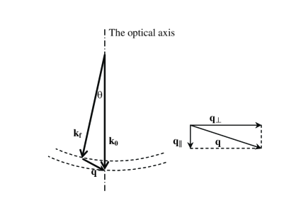
Figure 1: In an inelastic scattering, the momentum transfer vector q is determined by the initial and final wave-vector k₀ and k_f. The angle between the two wave vectors is defined as the scattering angle $\theta$. In the parallel illumination case, $\theta$ always equals to $\beta$ defined as the angle between the wave vector of scattering electrons $k_{f}$ and the optical axis.

A related problem also exists in other forms of spectroscopy. For instance, in solid state nuclear magnetic resonance (NMR), the signal depends strongly on the specimen orientation and more useful information is obtained after the discovery of the magic angle spinning nuclear magnetic resonance (MAS-NMR) methodRahman (1986); Andrew et al. (1959); Lowe (1959). Another example in XAS is the so-called ’magic angle’ condition used to eliminate the orientation effect for anisotropic systemsSt$\ddot{o}$hr (1992); Kiningsberger and Prins (1988). In EELS, the applied field responsible for electronic excitation is parallel to the direction of the momentum transfer vector q of the incident electron in the inelastic scatteringEgerton (1996). As shown in fig.1, by virtue of electron scattering, the direction of q is a function of the electron scattering angle $\theta$, being parallel to the incident electron beam at the zero scattering angle and changing towards a direction perpendicular to the beam with the increasing scattering angle.

In the angular integrated energy-loss spectroscopy with a centered circular aperture, a standard EELS collection condition particularly for high spatial resolution and high signal to noise ratio, electronic excitations of different momentum transfer q are recorded. Excitations induced by the applied fields over a range of directions are summedBrowning et al. (1991, 1993); Botton et al. (1995); Menon and Yuan (1998). Menon and YuanMenon and Yuan (1998) showed both experimentally and theoretically there also exists a magic angle (MA) at which the EELS signal is independent of specimen orientation. Their theory predicts the magic angle for a parallel beam illumination (MA_∥) to be $4\theta_{E}$. There $\theta_{E}$ is the characteristic angle which has a approximate form ${\theta}$_E=2E/E₀ (the more accurate definition is given by Ritchie and HowieRitchie and Howie (1977)) and with E being the energy-loss and E₀ the incident energy of the fast electrons. The derivation is for uniaxial, graphite-like, systems.

A number of other studies have also analyzed this problem again, mostly for uniaxial anisotropic systems. However, controversy as to the precise magic angle condition persists. For example, Zhu et al.Zhu et al. (1993) used an approximate method to arrive at a value of MA_∥ of about 1.8${\theta}$_E. Paxton et al.Paxton et al. (2000) used a different approach to arrive at MA_∥=1.36 ${\theta}$_E. Compounding this state of confusion in magic angle prediction is the report of Daniels et al.Daniels et al. (2003) who found experimentally that MA_∥=2${\theta}$_E and also provided a theoretical justification for their result. Souche et al.Souche et al. (1998) presented a more through theoretical analysis of the anisotropic electron energy-loss spectroscopy for graphite-like materials, taking into account the convergence beam effect. Their result for the parallel beam illumination is in agreement with the prediction of Menon and YuanMenon and Yuan (1998). In addition, apart from attempts by Paxton, all theoretical analysis has been confined to MAEELS in uniaxial systems, the applicability of the magic angle concept in more complex anisotropic systems is an unexplored area.

In order to make use of MAEELS, it is vital to understand the discrepancies between the various theories, particularly given that all models make the same basic assumptions, i.e. the electron beam scattering being kinetic, non-relativistic, and obeying the dipole approximation. In the process, we have demonstrated that the magic angle is a general effect which can occur in all sorts of anisotropic systems, be they crystalline, amorphous, single phase or nanostructured and applies to anisotropic transition whether it is intrinsic or extrinsic (for example, shape-effect induced).

The paper is organized as follows. In section II, we present a through analysis of electron energy-loss spectroscopy in anisotropic systems in order to establish a solid foundation for MAEELS in the core-electron excitation region and we derive a general definition for magic angle conditions. In section III, we show that the spectral information obtained at the magic angle is equivalent to orientationally averaged spectroscopy. From this geometrical interpretation, we can understand the different approaches used in MAEELS analysis reported in the literature and explain the reasons for discrepancies in the prediction of magic angle conditions. In section IV, we have provided more explicit MAEELS expressions for applications in specific material systems. In particular, we concentrated on more commonly encountered uniaxial and biaxial systems and establish the connection between MAEELS and other forms of magic angle spectroscopies such as XAS and MAS-NMR.

II Generalized MAEELS Theory

There are two ways to study the electronic excitation in anisotropic systems: the macroscopic approach is to use the dielectric function and the microscopic approach to calculate directly the quantum mechanical transition matrix element. Both approaches have been reported in the literatureZhu et al. (1993); Souche et al. (1998); Browning et al. (1991, 1993); Paxton et al. (2000); Daniels et al. (2003); Gloter et al. (2000) and physically they should yield the same result. To facilitate comparison of these reports, we will make our derivation using both approaches. It is known that the quantum mechanical approach can reveal the microscopic physics involved, but because of the need for accurate wave functions, it does not always yield useful experimental results. On the other hand, the dielectric approach is a phenomenological description of materials response that can be measured accurately, even though the microscopic origin of the electronic transitions may be obscuredVast et al. (2002).

II.1 Dielectric Formalism

Here we start with the dielectric approach where the calculation is relatively straightforward, because the information required is not the detailed excitation form of but the overall effect in terms of the response to a perturbation deserved by the relationJackson (1984):

$$D_{i}=\sum_{j}\varepsilon_{0}\varepsilon^{ij}E_{j}$$ (1)

where D, the electric displacement, is related to the electric field E by the well-known $\varepsilon^{ij}$ the dielectric function of the material system. $\varepsilon^{ij}$ is a ’metric tensor’Prince (1994), defined in terms of a reference frame where the orthogonal principle axes are aligned with the major symmetry directions of the physical system. For convenience, we have defined this reference frame as the sample frame (x,y,z).

The imaginary parts of (-1/$\varepsilon$) is known as the energy-loss functionEgerton (1996); Browning et al. (1991, 1993); Menon and Yuan (1998), providing a complete description of the response of the medium through which the fast electron is travelling. The double differential cross section used to estimate the intensity of EELS in an anisotropic system can be expressed asEgerton (1996); Browning et al. (1993):

$$\frac{d\sigma^{2}(\textbf{q})}{dEd\Omega}=\frac{4m_{e}}{na_{0}h^{2}}\textbf{\emph{Im}}(-\frac{1}{{\displaystyle\sum_{i,j}}q_{i}\varepsilon^{ij}q_{j}})$$ (2)

where m_e the mass of the fast electron and q is the momentum transfer vector of the fast electrons in the inelastic scattering process (see fig.1), n the number of atoms per unit volume of the material, a₀ the Bohr atomic radius, h the Plank constant and q_i the projection of q in the sample frame. Note the components of the dielectric function are assumed not to be a function of q, and this assumption corresponds to the dipole approximation in the quantum mechanical analysis of single electron transitionsJackson (1984).

We will restrict our discussion to core electron excitations in which we use the approximationEgerton (1996); Browning et al. (1991, 1993) for $\varepsilon_{1}$=Re($\varepsilon$) and $\varepsilon$₂=Im($\varepsilon$), $\varepsilon$₁ $\approx 1$ and $\varepsilon$₂ $\approx 0$. Eq.(2) can then be simplified to

$$\frac{d\sigma^{2}(\textbf{q})}{dEd\Omega}=\frac{4m_{e}}{na_{0}h^{2}}\sum_{i,j}\frac{q_{i}\varepsilon{{}_{2}}^{ij}q_{j}}{q^{4}}$$ (3)

From now on, we will be only interested in the EELS which is obtained by integrating Eq.(3) over the angular range determined by the collection condition, i.e. the convergence semi-angle $\alpha_{0}$ for a convergent beam and the collection semi-angle $\beta_{0}$ for the centered collection aperture used. This gives the partial angular integrated cross section

$$\frac{d\sigma}{dE}(\alpha_{0},\beta_{0},\widetilde{O})=\frac{4m_{e}}{na_{0}h^{2}}\sum_{i,j}(\int d\Omega\frac{q_{i}q_{j}}{q^{4}})\varepsilon{{}_{2}}^{ij}=\frac{8\pi m_{e}}{na_{0}h^{2}k_{0}^{2}}\sum_{i,j}W_{ij}(\alpha_{0},\beta_{0},\widetilde{O})\varepsilon{{}_{2}}^{ij}$$ (4)

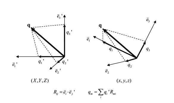
Figure 2: The projection of the momentum transfer vector q in the sample frames (x,y,z) and in the laboratory frame (X,Y,Z). The components $q_{i}$ ($q_{i}$’) are equivalent to q$\cdot$$\textbf{e}_{i}$ (q$\cdot$$\textbf{e}_{i}$’), where the $\textbf{e}_{i}$ ($\textbf{e}_{i}$’) are the basis vectors of the reference frame. Two sets of components of q are related by the transformation matrix R whose elements are defined in terms of dot product of the basis vectors of the two reference frames.

where $\widetilde{O}$ denotes the orientation of the sample with respect to the electron beam direction. Here the weighting factor W_ij depends both on the specimen orientation and the experimental condition used, i.e. $\alpha_{0}$ and $\beta_{0}$. In order to separate out these two effects, we have transformed the representation of q from the (x,y,z) orthogonal coordinate of the sample frame to the (X,Y,Z) orthogonal coordinate of the laboratory frame, with the Z axis defined to be optical axis of the electron beam. We denote the components of q in the (X,Y,Z) frame as q’_i(fig.2). Two representations of q are related to each other through the rotational transformation matrix R as:

$$q_{m}=\sum_{i}q^{\prime}_{i}R_{mi}$$ (5)

For transformation between two orthogonal coordinate systems, the rotational matrix element R_ij is defined to be the direction cosine between the basis vector e’ in the (X,Y,Z) frame and the basis vector e in the (x, y, z) frameJuretschke (1974); Prince (1994):

$$R_{ij}=\textbf{e}_{i}\cdot\textbf{e}_{j}^{\prime}$$ (6)

Substituting Eq.(5) into Eq.(4), we get the definition for the weighting factor as:

$$W_{ij}(\alpha_{0},\beta_{0},\widetilde{O})=\frac{k_{0}^{2}}{2\pi}\sum_{m,n}(\int d\Omega\frac{q_{m}^{\prime}q_{n}^{\prime}}{q^{4}})R_{mi}R_{nj}$$ (7)

In this way we have successfully separated out the orientation factors, in the form of the product of matrix elements, from the integral within the bracket which is solely determined by the experimental set-up. By inspection, we can see that the integration over the full azimuthal angle of vector q of the integrand with the cross-indices vanishes because of the rotational symmetry. This means that the integral has the simplified forms as follows:

$$\int d\Omega\frac{q_{m}^{\prime}q_{n}^{\prime}}{q^{4}}=\left\{\begin{array}[]{l@{}l}\displaystyle\int d\Omega\frac{q_{\parallel}^{2}}{q^{4}}=\frac{2\pi}{k_{0}^{2}}\xi_{\parallel}(\alpha_{0},\beta_{0})&(m=n=3)\\ \displaystyle\frac{1}{2}\int d\Omega\frac{q_{\perp}^{2}}{q^{4}}=\frac{2\pi}{k_{0}^{2}}\xi_{\perp}(\alpha_{0},\beta_{0})&(m=n=1or2)\\ \displaystyle 0&(m\neq n)\end{array}\right.$$ (11)

where we have introduced notation q_∥ and q_⟂ to denote the components of q that are parallel and perpendicular to the incident beam direction respectively (fig.1) and k₀ is the magnitude of the wave-vector for the fast electron beam. The factor $\displaystyle\frac{2\pi}{k_{0}^{2}}$ is used to eliminate the dimension of the reduced integral variable $\xi_{\parallel}$ and $\xi_{\perp}$.

Putting the integral expression in Eq.(11) back into Eq.(7) the weighting factor can be written as:

$$W_{ij}(\alpha_{0},\beta_{0},\widetilde{O})=\xi_{\parallel}R_{3i}R_{3j}+\xi_{\perp}(R_{1i}R_{1j}+R_{2i}R_{2j})$$ (12)

If we rearrange the product of the matrix element by applying the orthogonal property of the transformation matrixJuretschke (1974) as $\sum\limits_{m}R_{mi}R_{mj}=\delta_{ij}$, and through explicit calculation using Eq.(6), we can obtain a more revealing definition for the weighting factor

$$W_{ij}(\alpha_{0},\beta_{0},\widetilde{O})=\xi_{\perp}\delta_{ij}+(\xi_{\parallel}-\xi_{\perp})\cos\chi_{i}\cos\chi_{j}$$ (13)

where the $\chi_{i}$ is the angle between the optical axis (the Z-direction) of the laboratory frame and the ith basis vector in the sample frame. It is clear that the second term in Eq.(13) gives the information about orientation of the sample, so the magic angle condition is defined by the relation

$$\xi_{\parallel}(\alpha_{0}^{MA},\beta_{0}^{MA})=\xi_{\perp}(\alpha_{0}^{MA},\beta_{0}^{MA})$$ (14)

Note that our derivation has not exploited any special symmetry properties of the dielectric function, for example, some specific symmetry property brought by a crystal structure. Hence the magic angle condition is valid for all anisotropic systems, i.e., it not only applies to single crystals, but also to amorphous materials, powders, or nanostructures as long as an effective dielectric function tensor can be defined and measured.

II.2 Quantum Mechanical Theory

The dielectric function approach is very useful in treating practical problems. However, to understand the microscopic origin of the electronic transition responsible, it is better to work explicitly in terms of a quantum mechanical theory. With the wide spread use of ab-initio quantum mechanical calculation methods, proper treatment of the electronic excitation will become be routineNelhiebel et al. (1999); Hebert-Souche et al. (2000); Schattschneider et al. (2001). It is vital to know how to relate them to measurements where specimen-orientation is an additional variable.

IN quantum mechanics the inelastic scattering of high energy electrons can be described adequately by the first Born approximation asBethe (1964); Inokuti (1971):

$$\frac{d\sigma^{2}(\textbf{q})}{dEd\Omega}=\frac{4}{a_{0}^{2}}\cdot\frac{1}{q^{4}}|\langle f|\exp(-i\textbf{q}\cdot\textbf{r})|i\rangle|^{2}$$ (15)

where a₀ is Bohr atomic radius, and vector r is the coordinate of the electrons in the sample, the initial and final states of which are represented by $\langle{i}|$ and $\langle f|$ , respectively. Since we have not considered the screening of the fast electron Coulomb potential by other electrons inside the material, this expression is only applicable to core electron excitations. Because of the inverse q-dependence, electron scattering is concentrated at small angles. We can then expand the matrix element in terms of q and only retain the first non-zero term which is the dipole approximationEgerton (1996), to obtain

$$\frac{d\sigma^{2}(\textbf{q})}{dEd\Omega}\approx\frac{4}{a_{0}^{2}}\cdot\frac{1}{q^{4}}|\langle f|\textbf{q}\cdot\textbf{r})|i\rangle|^{2}=\frac{4}{a_{0}^{2}}\sum_{i,j}\frac{q_{i}q_{j}}{q^{4}}\langle x_{i}\rangle\langle x_{j}\rangle^{*}$$ (16)

After projecting q in the sample frame (x,y,z) mentioned above, one can see the connection between Eq.(16) and Eq.(4) by identifying $Im(\varepsilon^{ij})\propto\langle x_{i}\rangle\langle x_{j}\rangle^{*}$. The rest of the derivation can follow the procedure used in the dielectric formalism. Thus, we should arrive at the same conclusion as Eq.(7), so the magic angle condition should be the same as Eq.(14), i.e. $\xi_{\parallel}=\xi_{\perp}$.

II.3 The solution of the Magic angle condition

The magic angle condition refers to the convergence and collection semi-angles, $\alpha_{0}$ and $\beta_{0}$ respectively, which define the experimental set-up where Eq.(14) is satisfied. We recall that the fast electron has the simple energy-momentum relation $E_{0}=\displaystyle\frac{\hbar^{2}k_{0}^{2}}{2m}$ so the energy-loss process must satisfy the following energy and momentum relations

$$E=E-E_{0}=\displaystyle\frac{\hbar^{2}(k_{0}^{2}-k_{f}^{2})}{2m}$$ (17)

$$\textbf{q}=\textbf{k}_{0}-\textbf{k}_{f}$$ (18)

or

$$q^{2}=k_{0}^{2}+k_{f}^{2}-2k_{o}k_{f}\cos{\theta}$$ (19)

The simplest test case for magic angle conditions is for an experimental set-up involving parallel beam illumination. In this case, the scattering angle involved ($\theta$) is just the function of the semi-angle ($\beta$), defined to be the angle between the wave vector of the scattered electrons and the electron optical axis. For an axially placed circular detector, the maximum and minimum values of the momentum transfer are given by:

$$q_{min}=k_{0}-k_{f}=k_{0}\theta_{E}$$ (20a)

$$q_{max}=k_{0}^{2}+k_{f}^{2}-2k_{0}k_{f}\cos{\beta_{0}}$$ (20b)

Using above expressions for q to calculate the integral, following Paxton et al.Paxton et al. (2000), one obtains the result for the reduced integrals defined in Eq.(11) as:

$$\xi_{\parallel}=A=\frac{1}{8}\frac{2m}{\hbar^{2}}\frac{E^{2}}{E_{0}}(\frac{1}{q_{min}^{2}}-\frac{1}{q_{max}^{2}})+\frac{1}{2}\frac{E}{E_{0}}\ln{\frac{q_{max}}{q_{min}}}+\frac{1}{8}\frac{\hbar^{2}}{2m}\frac{1}{E_{0}}(q_{max}^{2}-q_{min}^{2})$$ (21a)

$$\xi_{\perp}=\frac{B-A}{2}=\frac{1}{2}(\ln{\frac{q_{max}}{q_{min}}-{\xi_{\parallel}})}$$ (21b)

This complex solution for the parallel beam illumination can be simplified because we are interested in the small-angle region where dipole approximation holds, so we can use the small angle approximation for q_⟂ ($\sim k_{0}\theta$) and q_∥ ($\sim q_{min}=k_{0}\theta_{E}$) as to obtain a more simplified form for the reduced integrals

$$\xi_{\parallel}=A\approx\frac{\hat{\beta}_{0}^{2}}{2(\hat{\beta}_{0}^{2}+1)}$$ (22a)

$$\xi_{\perp}=\frac{B-A}{2}\approx\frac{1}{4}[\ln(1+\hat{\beta}_{0}^{2})-\frac{\hat{\beta}_{0}^{2}}{\hat{\beta}_{0}^{2}+1}]$$ (22b)

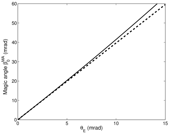
Figure 3: The magic angle is a function of the $\theta_{E}$ in the parallel illumination case under the small angle approximation, i.e. $\beta_{0}^{MA}$=$3.97\theta_{E}$(dashed), and for cases no limited by the small angle approximation(solid), i.e. solution of Eq.(14) and (21).

where we have used the reduced collection angle $\hat{\beta}_{0}=\beta_{0}/\theta_{E}$. We can solve the magic angle condition using the magic angle relation $\xi_{\parallel}=\xi_{\perp}$ i.e. $B=3A$. Within the small angle approximation, this is satisfied for $\beta_{0}^{MA}=3.97\theta_{E}$, or 4$\theta_{E}$ approximately as shown initially for a uniaxial systemMenon and Yuan (1998). In fig.3, the magic angle solution for the parallel beam illumination set-up is plotted as a function of $\theta_{E}$. The small-angle solution is found to be acceptable for the normal energy-loss and collection condition as the deviation from the more exact solution obtained from Eq.(21) and (22) is less than 5 percent.

II.4 Convergence angle effect

In many cases, explicitly for a focused probe system or implicitly because of the need to increase the illumination level at the sample using a slightly convergent beam, the magic angle solution for the parallel illumination condition becomes inapplicable. To take into account the convergence effect, we need to reexamine the momentum conservation relation shown in Eq.(19). This vector relation can be decomposed according to the vector components parallel and perpendicular to the electron optical axis. In the small-angle approximation (see fig.4), the parallel version of this relation is a scala equation:

$$\ q_{\parallel}\equiv-q_{Z}=k_{0}\theta_{E}$$ (23)

and perpendicular components of q are defined as follows:

$$\left\{\begin{array}[]{l}q_{X}=k_{0}(\alpha\cos\phi-\beta\cos\varphi)\\ q_{Y}=k_{0}(\alpha\sin\phi-\beta\sin\varphi)\\ q_{\perp}^{2}=q_{X}^{2}+q_{Y}^{2}=k_{0}^{2}\theta^{2}\\ \end{array}\right.$$ (27)

where $\phi$ and $\varphi$ are azimuth angles for wave-vectors of the incident and scattered electrons respectively and $\theta$ is the scattering angle between the direction of the incident electron and that of the scattered electron. The latter is related to $\alpha$ ($\beta$), the angle between the incident (scattered) electron and the electron beam axis, by spherical trigonometry:(see appendix)

$$\theta^{2}(\alpha,\beta,\phi-\varphi)=\alpha^{2}+\beta^{2}-2\alpha\beta\cos(\phi-\varphi)$$ (28)

Then, the reduced integral defined in Eq.(11) has the following form:

$$\xi_{\parallel}=A^{\prime}$$ (29a)

$$\xi_{\perp}=\frac{B^{\prime}-A^{\prime}}{2}$$ (29b)

where

$$A^{\prime}=\frac{1}{2\pi^{2}\alpha_{0}^{2}}\int_{0}^{\alpha_{0}}\alpha d\alpha\int_{0}^{2\pi}d\phi\int_{0}^{\beta_{0}}\beta d\beta\int_{0}^{2\pi}d\varphi\frac{\theta_{E}^{2}}{[\theta_{E}^{2}+\theta^{2}(\alpha,\beta,\phi-\varphi)]^{2}}$$ (30a)

$$B^{\prime}=\frac{1}{2\pi^{2}\alpha_{0}^{2}}\int_{0}^{\alpha_{0}}\alpha d\alpha\int_{0}^{2\pi}d\phi\int_{0}^{\beta_{0}}\beta d\beta\int_{0}^{2\pi}d\varphi\frac{1}{\theta_{E}^{2}+\theta^{2}(\alpha,\beta,\phi-\varphi)}$$ (30b)

The integral can be evaluated directly as an explicit function of the convergence and collection angles as:

$$A^{\prime}(\alpha_{0},\beta_{0},\theta_{E})=\frac{1}{4\hat{\alpha_{0}^{2}}}(D-C)$$

$$B^{\prime}(\alpha_{0},\beta_{0},\theta_{E})=\frac{1}{4\hat{\alpha_{0}^{2}}}\left\{[2\hat{\beta}_{0}^{2}\ln\frac{D+C-2\hat{\alpha_{0}^{2}}}{2}+2\hat{\alpha}_{0}^{2}\ln\frac{D+C-2\hat{\beta_{0}^{2}}}{2}]-(D-C)\right\}$$

where

$$C=\sqrt{-4\hat{\alpha}_{0}^{2}\hat{\beta}_{0}^{2}+(1+\hat{\alpha}_{0}^{2}+\hat{\beta}_{0}^{2})^{2}}$$

$$D=\hat{\alpha}_{0}^{2}+\hat{\beta}_{0}^{2}+1$$

$$\hat{\alpha}_{0}={\alpha_{0}}/{\theta_{E}}$$

$$\hat{\beta}_{0}={\beta_{0}}/{\theta_{E}}$$

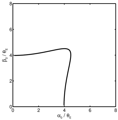
Figure 5: The contour expression for magic angles condition in electron energy loss spectroscopy of anisotropic core electron excitation.

Thus the solution of Eq.(14) is equivalent to $B^{\prime}=3A^{\prime}$. Eq.(29) is equivalent to Eq.(22) when the convergence angle $\alpha_{0}$ approaches zero. The numerical result is plotted as a contour in fig.5. Our result agrees with the result given by Souce et al Souche et al. (1998) in their determination for an uniaxial system through more tedious integration. It is worth pointing out that an earlier prediction by Menon and YuanMenon and Yuan (1998) for the magic angle condition in the convergent beam case is incorrect because it did not perform the actual azimuthal angular integration for both the incident beam and the scattered beam.

A striking feature of the solution shown above is the symmetry, that is, the interchangeability between the beam convergence range $\alpha_{0}$ of the incident electron and angular range $\beta_{0}$ of the collection of scattered electrons. This is already evident in Eq.(28). This can be traced to the small-angle approximation. Fig.4 shows that the surface of the Edward sphere described by the fast electrons becomes a plane of constant energy in the small angle approximation. It has been argued that dependence on $\alpha_{0}$ and $\beta_{0}$ are thus not symmetricalMenon and Yuan (1998), because the interchange of $\alpha$ and $\beta$ produces another momentum transfer vector which has the same parallel vector component but with a perpendicular component which is pointing in the opposite direction. Thus in the general case, the interchangeability of the convergence and the collection angles may not be valid . But in angular integrated spectroscopy, and in the small angle approximation, cross-section depends only on the modular square of q(see Eq.(11)), hence the interchangeability holds.

III Discussion of the theoretical model

Our theoretical analysis not only gives us a definition of the magic angle conditions, valid for an arbitrary anisotropic system, but it can also give a general expression for electron energy loss spectroscopy in anisotropic systems. This allows us to investigate in more detail the physical meaning of the magic angle conditions as well as understanding the discrepancy between the various reported magic angle analyses.

III.1 General expression for anisotropic EELS

A general expression for anisotropic EELS can be worked out by substituting the result of Eq.(13) back into Eq.(4). This gives the cross-section for the partially angular integrated electron energy-loss spectrum for core electron excitation in any anisotropic material systems in terms of their macroscopic dielectric function as:

$$\frac{d\sigma}{dE}(\alpha_{0},\beta_{0},\widetilde{O})=\frac{8\pi m_{e}}{na_{0}h^{2}k_{0}^{2}}[\xi_{\perp}\emph{{Im}}[Tr(\varepsilon)]+(\xi_{\parallel}-\xi_{\perp})\sum_{i,j}\cos\chi_{i}\cos\chi_{j}\varepsilon{{}_{2}}^{ij}]$$ (31)

As the trace of the dielectric function ’metric tensor’ Tr($\varepsilon)$ (=$\displaystyle\sum_{j}\varepsilon^{jj}$) is invariant with respect to rotational transformation, the first part of the expression does not change with specimen orientation. The second part has a pre-factor that vanishes at the magic angle conditions. So the cross-section for core electron excitation using MAEELS is

$$\frac{d\sigma}{dE}(\alpha_{0}^{MA},\beta_{0}^{MA})=\frac{8\pi m_{e}}{na_{0}h^{2}k_{0}^{2}}\xi_{\perp}^{MA}\emph{{Im}}[Tr(\varepsilon)]$$ (32)

III.2 Physical meaning of the magic angle effect

Another way to write Eq.(31) is as follows:

$$\frac{d\sigma}{dE}(\alpha_{0},\beta_{0},\widetilde{O})=\frac{8\pi m_{e}}{na_{0}h^{2}k_{0}^{2}}\left\{({\xi_{\parallel}+2\xi_{\perp}})\frac{\emph{{Im}}[Tr(\varepsilon)]}{3}+(\xi_{\parallel}-\xi_{\perp})\sum_{i,j}(\cos{\chi_{i}}\cos\chi_{j}-\frac{1}{3}\delta_{ij})\varepsilon^{ij}_{2}\right\}$$ (33)

As before, the factor $(\xi_{\parallel}-\xi_{\perp})$ gives the magic angle condition. However, if we rotate the crystal over all possible orientations($\widetilde{O}$), the averaged value of the angular dependent factors can be written asPrince (1994):

$$\overline{(\cos{\chi_{i}}\cos\chi_{j})}=\frac{1}{3}\delta_{ij}$$ (34)

This means that the second term in Eq.(33) drops out when the cross section is averaged over all the orientation, even if the magic angle condition is not satisfied, i.e.

$$\overline{\frac{d\sigma}{dE}}(\alpha_{0},\beta_{0})=\frac{8\pi m_{e}}{na_{0}h^{2}k_{0}^{2}}\left\{({\xi_{\parallel}+2\xi_{\perp}})\frac{\emph{{Im}}[Tr(\varepsilon)]}{3}\right\}$$ (35)

Thus we demonstrated that the spectrum obtained at magic angle condition is equivalent to that obtained by orientational averaging. This reason can be explained mathematically as follows.

In normal orientational averaging, the orientation can refer either to that of the specimen or the orientation of the external perturbation, i.e. the orientation of the applied field defined by the momentum transfer vector q in EELS. We can distinguish the averaging over the azimuth angle from 0 to 2$\pi$ , from averaging over the polar angle form 0 to $\pi$. In MAEELS, the azimuth angle averaging is achieved by using an axially placed circular detector. The remaining orientational averaging of q over the full polar angle range is not possible to achieve in EELS experiments, but the equivalent result may be obtained by integrating over a limited range of polar angles because electron scattering is skewed towards the small angle. However, it is not always possible to find the appropriate polar angular range, hence the magic angle condition is not trivial.

III.3 Comparison with other analysis

Now we can compare our prediction for the magic angle value with other derivations (see table.1) and to analysis the reasons for the diversity of the values predicted.

Menon and YuanMenon and Yuan (1998) and Souche et alSouche et al. (1998) both derived their values by working out the anisotropic spectral response in the uniaxial system, but otherwise their conclusions are identical with ours. Our general result is in agreement with their prediction for the specific uniaxial system.

Most interesting is that of Paxton et al. Paxton et al. (2000) who tried to derive a general theory for the magic angle condition. In their paper, the momentum transfer vector q is projected in the laboratory frame (X, Y, Z) defined above, so we have the quantum mechanical transitional matrix element as:

$${|\langle f|\textbf{q}\cdot\textbf{r})|i\rangle|^{2}}=|\langle f|q_{X}X+q_{Y}Y+q_{Z}Z|i\rangle|^{2}$$

$$=q_{X}^{2}\langle X\rangle^{2}+q_{Y}^{2}\langle Y\rangle^{2}+q_{Z}^{2}\langle Z\rangle^{2}+2q_{X}q_{Y}\emph{{Re}}[\langle X\rangle\langle Y\rangle^{*}]+2q_{Y}q_{Z}\emph{{Re}}[\langle Y\rangle\langle Z\rangle^{*}]+2q_{Z}q_{X}\emph{{Re}}[\langle Z\rangle\langle X\rangle^{*}]$$ (36)

where $\langle X\rangle^{2}=|\langle f|X|i\rangle|^{2}$, and $\langle X\rangle=|\langle f|X|i\rangle|$, the $\langle Y\rangle^{2}$, $\langle Z\rangle^{2}$, $\langle Y\rangle$ and $\langle Z\rangle$ have the similar definition. As discussed above, using the weighting given in Eq.(11), the angular integrated cross section can be written as:

$${\frac{d\sigma}{dE}(\alpha_{0},\beta_{0},\widetilde{O})\propto}\quad\xi_{\perp}\cdot(\langle X\rangle^{2}+\langle Y\rangle^{2})+\xi_{\parallel}\cdot\langle Z\rangle^{2}$$ (37)

If $\xi_{\perp}=\xi_{\parallel}=\xi_{0}$,then we have:

$${\frac{d\sigma}{dE}(\alpha_{0}^{MA},\beta_{0}^{MA})\propto}\quad\xi_{0}\cdot(\langle X\rangle^{2}+\langle Y\rangle^{2}+\langle Z\rangle^{2})$$ (38)

Paxton et al. Paxton et al. (2000) derived the magic angle condition by insisting that the isotropic spectra are given by this equation without giving detailed explanation. To show that it is orientation independent, we first consider a case where the specimen frame coincides with the lab frame, then

$$\langle X\rangle^{2}+\langle Y\rangle^{2}+\langle Z\rangle^{2}=\langle x\rangle^{2}+\langle y\rangle^{2}+\langle z\rangle^{2}$$ (39)

As the latter is proportional to the trace of the imaginary part of the dielectric function, it is invariable to rotation. So Paxton et al. Paxton et al. (2000) chose the correct magic angle condition, and should arrive at the same value for the magic angle as we do. But for reasons we could not understand, they concluded that the MA_∥ is about 1.36${\theta}$_E. We believe that it is a trivial mistake.

Daniels et al.’s derivationDaniels et al. (2003) has some similarity with our Eq.(36), but they have used the substitution in the beam direction coordinate (X,Y,Z) as:

$$\left\{\begin{array}[]{c}q_{X}=q_{XY}\cos{\phi}\\ q_{Y}=q_{XY}\sin{\phi}\end{array}\right.$$ (42)

$$\left\{\begin{array}[]{c}X=r_{XY}\cos{\phi}^{\prime}\\ Y=r_{XY}\sin{\phi}^{\prime}\end{array}\right.$$ (45)

where the r_XY was defined as the magnitude of vector r_XY-the position vector of the sample electron in the X-Y plane where the collection aperture lies, and q_XY has a similar definition. However, Daniels et al assumed that $\phi\neq\phi^{\prime}$, so their subsequent calculation can not be correct.

Zhu et al.Zhu et al. (1994) correctly recognized the importance of the rotationally symmetry of the experimental set-up, i.e. that the cross term as shown in Eq.(11) should vanish in integrating over azimuthal angle, so they focused on estimating the weighting of the cross-section along the polar angular range as:

$$\bar{q}_{\parallel}=\bar{q}_{\perp}$$ (46)

where $\displaystyle\bar{q}_{i}=\int q_{i}(\frac{d^{2}\sigma}{dEd\theta})d\Omega/\int(\frac{d^{2}\sigma}{dEd\theta})d\Omega$. The normalization factor in the denominator is just the equivalent expression for the isotropic system and we can define it as N. In the small angle approximation, we have:

$$\bar{q}_{\parallel}=\frac{k_{0}}{N}\int_{o}^{2\pi}d\varphi\int_{0}^{\beta_{0}}\theta d\theta\frac{\theta_{E}}{(\theta^{2}+\theta_{E}^{2})}$$ (47a)

$$\bar{q}_{\perp}=\frac{k_{0}}{N}\int_{o}^{2\pi}d\varphi\int_{0}^{\beta_{0}}\theta d\theta\frac{\theta}{(\theta^{2}+\theta_{E}^{2})}$$ (47b)

In fact $q_{\perp}=k_{0}\bar{\theta}$ where $\bar{\theta}$ is the so called mean scattering angle defined in Egerton’s book Egerton (1996), and has a value $\bar{\theta}=2\theta_{E}({\hat{\beta}_{0}-\arctan{\hat{\beta}_{0}}})/{\ln(\hat{\beta}_{0}^{2}+1)}$, and $q_{\parallel}=k_{0}{\theta_{E}}$. i.e. in his definition $\bar{\theta}=\theta_{E}$ and we can be resolve $\beta^{MA}_{0}\approx 1.76\theta_{E}$ according to this relation. For comparison, our equivalent integrals defined in Eq.(11) and (14) can be rewritten under the small angle approximation as:

$$\xi_{\parallel}=\int_{0}^{\beta_{0}}\theta d\theta\frac{\theta_{E}^{2}}{(\theta^{2}+\theta_{E}^{2})^{2}}$$ (48a)

$$\xi_{\perp}=\frac{1}{2}\int_{0}^{\beta_{0}}\theta d\theta\frac{\theta^{2}}{(\theta^{2}+\theta_{E}^{2})^{2}}$$ (48b)

Thus the guess of Zhu et al is incorrect numerically. By a similar argument, Gloter et alGloter et al. (2000) guessed a different weighting of transition with q parallel the beam direction and roughly estimated it with (q$\cdot$k₀)²/q²$k_{0}$². They also used the isotropic angular distribution as normalized factor. Remarkably, their guess is correct for parallel illumination case, but their expression can not correctly account for the convergence effect because it does not consider the scattering when the incident and scattered electron beams are not in the same plane as the beam optical axis.

In summary, we have analyzed the reasons for different prediction of magic angle values, and found all the discrepancies can be properly accounted for. This suggests that there is no fundamental objections to our theoretical model.

We will discuss the discrepancy between the experimental measurementDaniels et al. (2003) and the theoretical predicted value of magic angle in elsewhere. We want to emphasis here that the discrepancy is not due to errors in the theoretical analysis, but rather because of the simplicity of the theoretical assumption or the experimental interpretation. We can list a number of factors that might modify the prediction in our model, such as non-dipole transitionSaldin and Yao (1990), coherent scattering effectNelhiebel et al. (1999), channelling effectLee et al. (2000), relativistic effectEgerton (1996); Fano (1956). But our analysis showed that they may affect the exact values of the magic angle, but not the conclusion that magic angle effect, if it exists, applies to all anisotropic systems and that the spectra collected under magic angle condition represents an orientation averaging.

IV Applications

IV.1 Cross sections in anisotropic systems

We will discuss special cases for the symmetries exemplified by crystalline systems, although in fact the systems can be amorphous or nanostructured. This allows us to write out the explicit form of the dielectric function, hence the precise form of the cross-section for the partially angular integrated EELS core loss excitation:

i) Isotropic systems

This category includes cubic crystals where the non-diagonal elements vanish and the diagonal elements are identical, of which the imaginary parts are set to be $\varepsilon_{2}$. So the cross section for EELS is given by:

$$\frac{d\sigma}{dE}=\frac{8\pi m_{e}}{na_{0}h^{2}k_{0}^{2}}\left\{[3\xi_{\perp}+(\xi_{\parallel}-\xi_{\perp})\sum_{i}\cos^{2}\chi_{i}]\varepsilon_{2}\right\}\equiv\frac{8\pi m_{e}}{na_{0}h^{2}k_{0}^{2}}(\xi_{\parallel}+2\xi_{\perp})\varepsilon_{2}$$ (49)

where we have used the relation $\displaystyle\sum_{i}\cos^{2}\chi_{i}=1$ Prince (1994). According to the definition of the reduced integral in Eq.(11), the factor $(\xi_{\parallel}+2\xi_{\perp})$ is in fact proportional to $\ln(\hat{\beta}_{0}^{2}+1)$ in the case of parallel illumination.

ii) Uniaxial systems

There are hexagonal, tetragonal and rhombohedral crystals in this class where the physical response is unique in one direction. The dielectric function is characterized by two different element as follows:

$$\varepsilon^{ij}=\left\{\begin{array}[]{r@{\quad}l}\varepsilon^{\parallel}&i=j=3\\ \varepsilon^{\perp}&i=j=1or2\\ 0&i\neq j\end{array}\right.$$ (53)

This means that the cross-section for EELS in this class of system is given by:

$$\frac{d\sigma}{dE}=\frac{8\pi m_{e}}{na_{0}h^{2}k_{0}^{2}}\left\{[\xi_{\perp}(1+\cos^{2}\chi_{3})+\xi_{\parallel}\sin^{2}\chi_{3}]\varepsilon_{2}^{\perp}+(\xi_{\parallel}\cos^{2}\chi_{3}+\xi_{\perp}\sin^{2}\chi_{3})\varepsilon_{2}^{\parallel}\right\}$$ (54)

iii) Orthorhombic systems

In this case, the dielectric function have three independent diagonal elements $\varepsilon^{jj}$, so we have:

$$\frac{d\sigma}{dE}=\frac{8\pi m_{e}}{na_{0}h^{2}k_{0}^{2}}\left\{\sum_{j}[\xi_{\perp}+(\xi_{\parallel}-\xi_{\perp})\cos^{2}\chi_{j}]\varepsilon_{2}^{jj}\right\}$$ (55)

iv) Monoclinic and Triclinic systems

The off-diagonal elements do not vanish in these systems, so we have:

$$\frac{d\sigma}{dE}=\frac{8\pi m_{e}}{na_{0}h^{2}k_{0}^{2}}\left\{\sum_{i,j}[\xi_{\perp}\delta_{ij}+(\xi_{\parallel}-\xi_{\perp})\cos\chi_{i}\cos\chi_{j}]\varepsilon_{2}^{ij}\right\}$$ (56)

IV.2 ’Magic’ orientation in the orthogonal systems

Here we concentrate on the most commonly encountered orthogonal system. The cross section Eq.(55) can be rearranged as:

$$\frac{d\sigma}{dE}=\frac{8\pi m_{e}}{na_{0}h^{2}k_{0}^{2}}\left\{\sum_{j}W_{jj}\varepsilon^{jj}_{2}\right\}=\frac{8\pi m_{e}}{na_{0}h^{2}k_{0}^{2}}\left\{({2\xi_{\perp}+\xi_{\parallel}})\frac{\emph{{Im}}[Tr(\varepsilon)]}{3}+(\xi_{\parallel}-\xi_{\perp})\sum_{j}(\cos^{2}\chi_{j}-\frac{1}{3})\varepsilon^{jj}_{2}\right\}$$ (57)

Again the first part is rotationally invariant so it represents the isotropic spectrum. The second part contains the information about the specimen rotation. The first bracket represents the factor responsible for the magic angle condition. The interesting point is the existence of other factors $(\cos^{2}\chi_{j}-1/3)$ inside the summation over j. This suggests that the second part will also vanish if all the brackets within the summation sign equal to zero. They uniquely define a specific specimen orientation ($\chi_{j}=54.7^{\circ}$) which we may label as the ’magic’ orientation. Again the spectrum so obtained equals that obtained at the magic angle condition or by through orientational averaging. This is understandable as $\cos\chi_{j}$ is the projection of the jth basis vector at the optical axis, so each principle symmetry electronic excitation contributes equally. By rotation symmetry about the beam direction, the same result holds for the more general case involving convergence illumination.

In uniaxial systems whose dielectric function has only two variables $\varepsilon_{\parallel}$ and $\varepsilon_{\perp}$ , the angular integrated cross section as shown in Eq.(54) becomes

$$\frac{d\sigma}{dE}=\frac{8\pi m_{e}}{na_{0}h^{2}k_{0}^{2}}\left\{({2\xi_{\perp}+\xi_{\parallel}})\frac{\varepsilon^{\parallel}_{2}+2\varepsilon^{\perp}_{2}}{3}+(\xi_{\parallel}-\xi_{\perp})(\cos^{2}\chi_{3}-\frac{1}{3})(\varepsilon^{\parallel}_{2}-\varepsilon^{\perp}_{2})\right\}$$ (58)

Clearly, the ’magic’ orientation defined above is reduced to a ’magic angle’ between the z-axis of the sample and the optical axis, i.e.$\chi_{3}=54.7^{\circ}$ in uniaxial system. However, we have distinguished this ’magic angle’ of specimen orientation with the magic angle for the beam convergence and collection in MAEELS.

In summary, the ’magic’ orientation can provide a set up at which the spectra should be the same as the spectra gained at the magic angle for the system where the symmetry is higher than orthogonal, and this ’magic’ orientation will lose its meaning in a system whose dielectric function has the non-zero off-diagonal elements.

Our analysis suggests that a better way to represent the anisotropic response of EELS is to write it as a linear combination of the orientationally averaged (also called ’isotropic’) spectrum and an orientation dependent spectrum. In uniaxial systems, the orientation-dependent spectrum can be further expressed as a product of the magic angle factor, the magic orientation factor and a dichroic spectrum:

$$\varepsilon_{2}|_{Anisotropic}=({2\xi_{\perp}+\xi_{\parallel}})\cdot\varepsilon_{2}|_{Average}+(\xi_{\parallel}-\xi_{\perp})(\cos^{2}\chi_{3}-\frac{1}{3})\cdot\varepsilon_{2}|_{Dichroic}$$ (59)

where

$$\varepsilon_{2}|_{Average}=\frac{2\varepsilon^{\perp}_{2}+\varepsilon^{\parallel}_{2}}{3}$$ (60a)

$$\varepsilon_{2}|_{Dichroic}=\varepsilon^{\parallel}_{2}-\varepsilon^{\perp}_{2}$$ (60b)

This formula should offer a practical way to study the anisotropy in the core electron excitation as well as encoding the magic angle and magic orientation conditions.

IV.3 Connections between MAS for EELS, for NMR and for XAS

The magic orientation effect has a direct analogue with the ’magic angle effect’ in XAS experiments and less directly with magic angle spinning nuclear magnetic resonance (MAS-NMR).

In surface extended x-ray absorption fine structure (SEXAFS)St$\ddot{o}$hr (1992); Kiningsberger and Prins (1988), one can study the bonding length as well as local coordination number of the excited atoms. However, contribution of more than one shell to the measured EXAFS can result in a polarization dependent measured distance from absorbing atom to the neighboring atoms and affect the effective coordinate number. If there is higher than twofold symmetry around the surface normal, the correct distance and the real coordinate number can be directly measured if the angle, between the electric field vector E of the incident x-ray and the surface normal of the single crystal, is equivalent to 54.7^∘ exactly. This is because the system being probed is effectively an uniaxial system.

Another famous example is the MAS-NMR technique for solidRahman (1986); Andrew et al. (1959); Lowe (1959). If the material, whether it is a single crystal, polycrystal or power, spun with high speed about an axis which is respect to the applied magnetic field with 54.7^∘ , the NMR result will be independent of the orientation of the sample. MAS-NMR is also related to the orientational magic angle effect because one is effectively using spinning to create an effective ’uniaxial system’ out of powered samples.

V Conclusion

We have presented a general model describing anisotropy of the core-level electron excitation in EELS measurement and have determined the magic angle condition at which the sample orientation becomes irrelevant. After comparing our derivation with reported theoretical efforts, we can explain all the reasons for disagreement in the literature predicting the value of the magic angle and showed that the differences in no way invalid our approach. Furthermore, for the first time, we showed that the magic angle condition is applicable in all anisotropic systems and that the spectrum at the magic angle condition is equivalent to the rotational average of the sample. The same analysis can also give the general expression for electron energy loss spectroscopy of core electron excitation in anisotropic system. In high symmetry cases, it leads to the discovery of the magic orientation condition. Its relation with other ’magic angle effect’ is clarified. In addition, the analysis shows that EELS in uniaxial system can be written as a sum of the effective ’isotropic’ spectrum and the linear dichroic spectrum.

Appendix A the geometrical explanation for Eq.(28)

The perpendicular component of the momentum transfer q can be seen as a sum of the perpendicular components of the initial and the final wave-vector in the case of the convergence beam as:

$$\textbf{q}_{\perp}={\textbf{k}_{0}}^{\perp}-{\textbf{k}_{f}}^{\perp}$$ (61)

According to the vector relations shown in fig.4 under the small angle approximation, we have:

$${q}_{\perp} = {k_{0}}\theta$$ (62)

$${k_{0}}^{\perp} = {k_{0}}\alpha$$ (63)

$${k_{f}}^{\perp} = {k_{0}}\beta$$ (64)

Thus the scattering angle $\theta$ can be written following the vector combination rule as:

$$\vec{\theta}=\vec{\alpha}-\vec{\beta}$$ (65)

where the directional properties of these angular vectors are defined to be the same as the perpendicular components of their corresponding wave-vectors. According to the law of cosines, the magnitude of $\vec{\theta}$ therefore can be written as: Eq.(28).

$$\theta(\alpha,\beta,\phi-\varphi)^{2}=\alpha^{2}+\beta^{2}-2\alpha\beta\cos(\phi-\varphi)$$

Table 1: The predicted values of the magic collection angle for the parallel illumination case.

Authors	ZhuZhu et al. (1994)	MenonMenon and Yuan (1998)	PaxtonPaxton et al. (2000)	SoucheSouche et al. (1998)	DanielsDaniels et al. (2003)
MA∥($\beta_{0}^{MA}/\theta_{E}$)	1.8	4	1.36	3.97	1.98

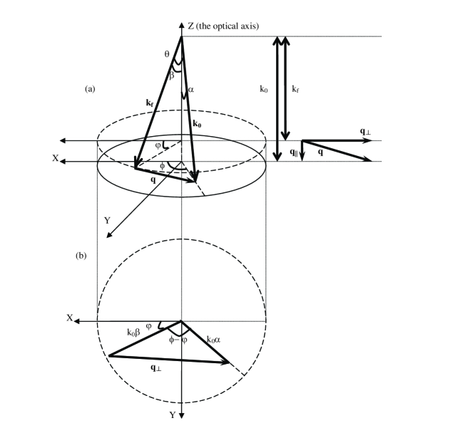
Figure 4: Schematic diagram of the inelastic scattering under the small angle approximation (a) and its projection in the plane perpendicular to the optical axis (b). The convergence angle effect has been taken into consideration.

References

- Juretschke (1974) H. Juretschke, Macroscopic Physics of Anisotropic Solids (W.A. Benjamin, Massachusetts, 1974).
- Leapman and Silcox (1979) R. Leapman and J. Silcox, Phys.Rev.Lett. 42, 1361 (1979).
- Leapman et al. (1983) R. Leapman, P. Fejes, and J. Silcox, Phys.Rev.B 28, 2361 (1983).
- Disko et al. (1982) M. Disko, O. Krivanek, and P. Rez, Phys.Rev.B 25, 4252 (1982).
- Baston (1993) P. Baston, Phys.Rev.B 48, 2608 (1993).
- Kiningsberger and Prins (1988) D. Kiningsberger and R. Prins, X-ray Absorption: Principles, Applications, Techniques of EXAFS, SEXAFS and XANES (A Wiley-Interscience Publication, New York, 1988).
- Sthr (1992) J. Sthr, NEXAFS Spectroscopy (Springer, Berlin, 1992).
- Egerton (1996) R. Egerton, Electron Energy Loss Spectroscopy in the Electron Microscope (Plenum Press, New York, 1996).
- Ruiter et al. (1997) A. G. T. Ruiter, J. A. Veerman, M. F. Garcia-Parajo, and N. F. van Hulst, J.Phys.Chem.A 101, 7318 (1997).
- van Hulst et al. (2000) N. F. van Hulst, J. A. Veerman, M. F. Garcia-Parajo, and L. Kuipers, J.Chem.Phys. 112, 7799 (2000).
- Rahman (1986) A. Rahman, Nuclear Magnetic Resonance: Basic Principles (Springer-Verlag, New York, 1986).
- Lee et al. (2000) Y. S. Lee, Y. Murakami, D. Shindo, and T. Oikawa, Mater. Trans., JIM 41, 555 (2000).
- Lubbe et al. (1999) M. Lubbe, P. R. Bressler, W. Braun, T. U. Kampen, and D. R. T. Zahn, J.Appl.Phys. 86, 209 (1999).
- Zhu et al. (1993) Y. M. Zhu, Z. Wang, and M. Suenaga, Philos.Mag.A 67, 11 (1993).
- Zhu et al. (1994) Y. M. Zhu, J. M. Zuo, A. R. Moodenbaugh, and M. Suenaga, Philos. Mag. A, Phys. Condens. Matter Defects Mech. Prop. 70, 969 (1994).
- Fink et al. (1994) J. Fink, N. Nucker, E. Pellegrin, H. Romberg, M. Alexander, and M. Knupfer, J. Electron Spectrosc. Rel. Phenom. 66, 395 (1994).
- Nucker et al. (1995) N. Nucker, E. Pellegrin, P. Schweiss, J. Fink, S. Molodtsov, C. Simmons, G. Kaindl, W. Frentrup, A. Erb, and G. Muller-Vogt, Phys.Rev.B 51, 8529 (1995).
- Zhu et al. (2002) Y. Zhu, A. R. Moodenbaugh, G. Schneider, J. W. Davenport, T. Vogt, Q. Li, G. Gu, D. A. Fischer, and J. Tafto, Phys.Rev.Lett. 88, 247002 (2002).
- Kong et al. (2002) X. Kong, Y. Q. Wang, H. Li, X. F. Duan, R. C. Yu, S. C. Li, F. Y. Li, and C. Q. Jin, Appl.Phys.Lett. 80, 778 (2002).
- Zhang et al. (2003) G. P. Zhang, G. S. Chang, T. A. Callcott, D. L. Ederer, W. N. Kang, E. M. Choi, H. J. Kim, and S. I. Lee, Phys.Rev.B 67, 174519 (2003).
- Klie et al. (2003) R. F. Klie, H. B. Su, Y. M. Zhu, J. W. Davenport, J. C. Idrobo, N. D. Browning, and P. D. Nellist, Phys.Rev.B 67, 144508 (2003).
- Souche et al. (1998) C. Souche, B. Jouffrey, and M. Nelhiebel, Micron 29, 419 (1998).
- Vast et al. (2002) N. Vast, L. Reining, V. Olevano, P. Schattschneider, and B. Jouffrey, Phys.Rev.Lett. 88, 037601 (2002).
- Andrew et al. (1959) E. Andrew, A. Bradbury, and R. Eades, Nature 183, 1802 (1959).
- Lowe (1959) I. Lowe, Phys.Rev.Lett. 2, 285 (1959).
- Browning et al. (1991) N. Browning, J. Yuan, and L. Brown, Ultramicroscopy 38, 291 (1991).
- Browning et al. (1993) N. Browning, J. Yuan, and L. Brown, Philos.Mag.A 67, 261 (1993).
- Botton et al. (1995) G. A. Botton, C. B. Boothroyd, and W. M. Stobbs, Ultramicroscopy 59, 93 (1995).
- Menon and Yuan (1998) N. K. Menon and J. Yuan, Ultramicroscopy 74, 83 (1998).
- Ritchie and Howie (1977) R. H. Ritchie and A. Howie, Philo.Mag. 36, 463 (1977).
- Paxton et al. (2000) A. T. Paxton, M. van Schilfgaarde, M. MacKenzie, and A. J. Craven, J.Phys.Cond.Mat. 12, 729 (2000).
- Daniels et al. (2003) H. Daniels, A. Brown, A. Scott, T. Nichells, B. Rand, and R. Brydson, Ultramicroscopy 96, 523 (2003).
- Gloter et al. (2000) A. Gloter, J. Ingrin, D. Bouchet, and C. Colliex, Phys.Rev.B 61, 2587 (2000).
- Jackson (1984) J. Jackson, Classical electrodynamics (Wiley, and Sons, New York, 1984).
- Prince (1994) E. Prince, Mathematical Techniques in Crystallography and Material Science (Springer-Verlag, Berlin, 1994).
- Nelhiebel et al. (1999) M. Nelhiebel, P. H. Louf, P. Schattschneider, P. Blaha, K. Schwarz, and B. Jouffrey, Phys.Rev.B 59, 12807 (1999).
- Hebert-Souche et al. (2000) C. Hebert-Souche, P. H. Louf, P. Blaha, M. Nelheibel, J. Luitz, P. Schattschneider, K. Schwarz, and B. Jouffrey, Ultramicroscopy 83, 9 (2000).
- Schattschneider et al. (2001) P. Schattschneider, C. Hebert, and B. Jouffrey, Ultramicroscopy 86, 343 (2001).
- Bethe (1964) H. Bethe, Intermediate Quantum Mechanics (Benjamin,W.A., New York, 1964), 1st ed.
- Inokuti (1971) M. Inokuti, Rev.Mod.Phys. 43, 297 (1971).
- Saldin and Yao (1990) D. Saldin and J. Yao, Phys.Rev.B 41, 52 (1990).
- Fano (1956) U. Fano, Phys.Rev. 102, 385 (1956).