Oscillations of the Electric-Dipole Echo in Glasses in a Magnetic Field

Abstract

Using a simple diagram technique we derive the electric-dipole echo amplitude from two-level systems with a quadrupole nuclear moment in glasses in an external magnetic field. We show, that due to the quadrupole moment interaction of a tunneling particle with a gradient of an internal electric field, the echo amplitude experiences oscillations in rather weak magnetic fields. With an increase of the magnetic field, when the Zeeman energy becomes larger than the quadrupole energy splitting, the average echo amplitude increases and saturates (for high magnetic fields) at some level which is above the average level of echo oscillations for small magnetic fields.

I INTRODUCTION

Recently it was experimentally observed that the electric-dipole echo amplitude in non-magnetic glasses oscillates as a function of applied magnetic field LESH ; LNHE . Similar behavior was found in insulating crystals with tunneling impurities EL . In a recent paper WFE such behavior was attributed to quadrupole nuclear moments of tunneling particles interacting with the magnetic field and with the gradient of an internal electric field. The purpose of this paper is to formulate a general microscopic theory of this phenomenon taking into account a multi-level structure of tunneling systems in glasses coupled with a quadrupole nuclear moment. To this end we have developed a simple diagram technique describing the coherent echo signal. Making use of this technique, one can easily generalize known results for the echo amplitude from the usual two-level systems (TLS) to more general multi-level systems.

II DIAGRAM REPRESENTATION OF THE ECHO

In this section we give a simple diagram representation of the two-pulse echo signal from an arbitrary multi-level system. We then apply this technique to a multi-level system formed by a TLS with a quadrupole nuclear moment. The microscopic details of the TLS-quadrupole interaction in glasses are discussed further down in the next section. First we start with a simple example of an echo in an ensemble of TLS. To avoid unnecessary complications we will use a simple perturbative approach regarding the applied electric field, similar to the one considered in Ref. GMP . However all results can easily be generalized to strong electric fields.

II.1 Echo in an Ensemble of TLS

The wave function of a TLS in an external ac-electric field is a linear combination of the wave functions $\varphi_{1}$ and $\varphi_{2}$ for each level

$$\Psi=C_{1}\varphi_{1}+C_{2}\varphi_{2},\qquad|C_{1}|^{2}+|C_{2}|^{2}=1.$$ (1)

Prior to the action of the first electric pulse we have $C_{1}=1$ and $C_{2}=0$. Then in the electric field the time variation of the amplitudes $C_{1}$ and $C_{2}$ obeys the equations

$$i\hbar\displaystyle\frac{dC_{1}}{dt}=E_{1}C_{1}+V(t)C_{2},\quad i\hbar\displaystyle\frac{dC_{2}}{dt}=E_{2}C_{2}+V(t)C_{1}.$$ (2)

For the off-diagonal transition matrix element $V(t)$ we have a following expression during the electric pulse

$$V(t)=V_{1,2}\cos\omega t,\quad\mbox{where}\quad V_{1,2}=({\bf F}_{1,2}\cdot{\bf m})\frac{\Delta_{0}}{E}.$$ (3)

Here ${\bf F}_{1,2}$ is the electric field amplitude of the first or the second electric pulse, respectively, ${\bf m}$ is the dipole moment of the TLS, $\Delta_{0}$ the tunneling splitting, $E=E_{2}-E_{1}$ the TLS energy, and $E_{1}$ and $E_{2}$ are the energies of the ground and the excited states of the TLS, respectively. The electric field frequency is assumed as $\hbar\omega\approx E$. To simplify our equations we will put $\hbar=1$.

After the action of the 1st electric pulse $C_{2}$ acquires in the first approximation a finite value proportional to amplitude $V_{1}$ which is assumed to be small. During the time interval between the first and second electric pulses ($0<t<\tau_{21}$) we have

$$C_{2}\propto(-iV_{1})\cdot e^{-iE_{2}t},\quad C_{1}\approx 1\cdot e^{-iE_{1}t}-O(V_{1}^{2}).$$ (4)

In Eq. (4) for $C_{2}$ we have omitted the resonance factor

$$\beta_{21}(\tau_{1})=\frac{1}{z}\sin\frac{z\tau_{1}}{2}\exp\left(-iE_{2}\tau_{1}+i\frac{z\tau_{1}}{2}\right),$$ (5)

where $\tau_{1}$ is a duration of the first pulse, and $z=E-\omega$ is a detuning from the resonance. For a transition between the second and the first level (under the action of the second pulse, see below) the corresponding resonance factor reads

$$\beta_{12}(\tau_{2})=-\frac{1}{z}\sin\frac{z\tau_{2}}{2}\exp\left(-iE_{1}\tau_{2}-i\frac{z\tau_{2}}{2}\right).$$ (6)

These resonance factors are very important in describing the form of the echo envelope GMP2 . But in the present paper we are mainly interested in the echo amplitude as a function of the time delay $\tau_{21}$ between the two pulses. To make our equations as simple as possible, we assume that $\tau_{21}$ is much larger than the duration of any pumping pulse, $\tau_{i}$. As we will show below, if the electric pulses $\tau_{i}$ are sufficiently short (the exact criterion for a TLS-quadrupole multi-level system will be given in the last section) such resonant factors are not important for our purposes and we will not take them into account in the following analysis (though they can easily be included if necessary).

Let us now discuss what happens just after the action of the second electric pulse $V_{2}\cos\omega t$. Using Eq. (2) we calculate the corresponding variations of $C_{1}$ and $C_{2}$:

$$\begin{array}[]{rcl}\delta C_{1}&\propto&(-iV_{2})\cdot C_{2}(\tau_{21})\propto(-iV_{2})\cdot(-iV_{1})e^{-iE_{2}\tau_{21}},\\[5.0pt] \delta C_{2}&\propto&(-iV_{2})\cdot C_{1}(\tau_{21})\propto(-iV_{2})\cdot e^{-iE_{1}\tau_{21}},\end{array}$$ (7)

(here for the reasons mentioned above we have omitted the resonance factors $\beta_{12}(\tau_{2})$ and $\beta_{21}(\tau_{2})$ in $\delta C_{1}$ and $\delta C_{2}$, respectively). Finally, at some moment $t$ after the 2nd pulse we have

$$\delta C_{1}\propto-V_{1}V_{2}e^{-iE_{2}\tau_{21}}\cdot e^{-iE_{1}(t-\tau_{21})},\quad\delta C_{2}\propto-iV_{2}e^{-iE_{1}\tau_{21}}\cdot e^{-iE_{2}(t-\tau_{21})}.$$ (8)

The amplitude of the two-pulse echo from one TLS is determined by the average value of the product $\delta C_{1}\delta C_{2}^{*}$ (i.e. by the off-diagonal density matrix element) which is proportional to

$$p_{\rm echo}\propto\delta C_{1}\delta C_{2}^{*}\propto-iV_{1}V_{2}^{2}e^{i(E_{1}-E_{2})\tau_{21}}\cdot e^{i(E_{2}-E_{1})(t-\tau_{21})}.$$ (9)

Summing over all resonant TLS we have for the two-pulse echo amplitude

$$P_{\rm echo}\propto-i\sum_{\rm TLS}V_{1}V_{2}^{2}e^{iE(t-2\tau_{21})}.$$ (10)

For $t=2\tau_{21}$ the amplitude of the echo has a sharp maximum, $P_{\rm echo}\propto-iV_{1}V_{2}^{2}\,N$, where $N$ is the number of resonant TLS (i.e. TLS with $\hbar\omega\approx E)$.

Let us now give a simple diagram representation of this result. It will allow us to generalize our approach to the more complicated case of an echo in a multi-level system formed, for example, by a tunneling particle with a quadrupole nuclear moment. For simplicity, we assume that the electric field amplitudes ${\bf F}_{1,2}$ of the two electric pulses are parallel to each other, i.e. ${\bf F}_{i}=F_{i}{\bf e}$, where ${\bf e}$ is a unit polarization vector. Then we have the following expression for the induced dipole moment echo amplitude from a single TLS

$$\begin{array}[]{ccc}p_{\rm echo}\propto(-iF_{1})\alpha_{21}\cdot e^{-iE_{2}\tau_{21}}\cdot(-iF_{2})\alpha_{12}\cdot e^{-iE_{1}(t-\tau_{21})}\cdot\left[e^{-iE_{1}\tau_{21}}\cdot(-iF_{2})\alpha_{21}\cdot e^{-iE_{2}(t-\tau_{21})}\right]^{*}\cdot\alpha_{21}=&&\\[10.0pt] =-iF_{1}F_{2}^{2}|\alpha_{12}|^{2}|\alpha_{21}|^{2}e^{i(E_{2}-E_{1})(t-\tau_{21})-i(E_{2}-E_{1})\tau_{21}}=-iF_{1}F_{2}^{2}|\alpha_{12}|^{2}|\alpha_{21}|^{2}e^{iE(t-2\tau_{21})}.\end{array}$$ (11)

Here $\alpha_{ij}$ are the off-diagonal dipole transition matrix elements projections on the direction of the electric field. In the considered case they are real quantities and given by the usual expression

$$\alpha_{12}=\alpha_{21}=({\bf e}\cdot{\bf m})\frac{\Delta_{0}}{E}.$$ (12)

Generally they obey the relations $\alpha_{12}=\alpha^{*}_{21}$.

Eq. (11) is similar to Eq. (9) and can be depicted by the diagram shown in Fig. 1.

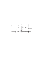
Figure 1: A diagram for a two-pulse echo from a TLS.

Each full or dashed vertical line in the diagram corresponds to a transition from level $i$ to level $k$ ($i,k=1,2$) under the action of the first or second electric pulse. To each vertical line we ascribe a factor $(-iF_{1,2})\alpha_{ki}$ (depending of the pulse). For example, the line $DA$ corresponds to the factor $(-iF_{1})\alpha_{21}$ and the full line $BE$ to the factor $(-iF_{2})\alpha_{12}$. The dashed line $EB$ corresponds to the factor $(-iF_{2})\alpha_{21}$. Finally the dotted line $FC$ (the echo signal) corresponds to the factor $\alpha_{21}$.

Each horizontal line in this diagram (full or dashed) corresponds to free TLS dynamics in the time intervals between or after the pulses. Therefore, an appropriate exponential factor is ascribed to each such line. The factor $\exp(-iE_{2}\tau_{21})$ corresponds to the line $AB$ and the factor $\exp(-iE_{1}\tau_{21})$ to line $DE$. The factors $\exp[-iE_{2}(t-\tau_{21})]$ and $\exp[-iE_{1}(t-\tau_{21})]$ are represented by the lines $BC$ and $EF$, respectively. In the final expression all factors corresponding to dashed lines should be taken as complex conjugated. It is easy to see that all full lines (vertical and horizontal) contribute to the amplitude $\delta C_{1}$ and all dashed lines to $\delta C_{2}$.

II.2 Echo in a Multi-Level System

Using these simple diagram rules we can now easily find the contributions to the two-pulse echo signal from a multi-level system. Let us, for example, consider a multi-level system as shown in Fig. 2.

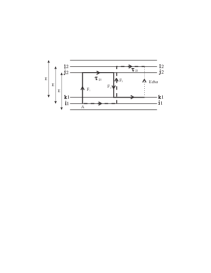
Figure 2: A diagram for the two-pulse echo from TLS-quadrupole multi-level system.

It consists of two identical groups of $N$ levels shifted vertically against each other by some energy $E$ (playing the role of the usual TLS energy). Inside the groups the positions of the levels are arbitrary, i.e. they are not necessarily equidistant. As we will see in the next section, such a multi-level system describes a TLS with a quadrupole nuclear moment.

According to the rules formulated above, the diagram in Fig. 2 gives the following partial contributions to the two-pulse echo signal

$$\begin{array}[]{ccc}\pi_{i1,k1,j2,l2}(t)=\frac{\displaystyle 1}{\sqrt{\displaystyle N}}(-iF_{1})\alpha_{j2,i1}\cdot e^{-iE_{j2}\tau_{21}}\cdot(-iF_{2})\alpha_{k1,j2}\cdot e^{-iE_{k1}(t-\tau_{21})}\times&&\\[10.0pt] \times\left[\frac{\displaystyle 1}{\sqrt{\displaystyle N}}e^{-iE_{i1}\tau_{21}}\cdot(-iF_{2})\alpha_{l2,i1}\cdot e^{-iE_{l2}(t-\tau_{21})}\right]^{*}\cdot\alpha_{\rm l2,k1}=&&\\[10.0pt] =-\frac{\displaystyle i}{\displaystyle N}F_{1}F_{2}^{2}\alpha_{j2,i1}\cdot\alpha_{k1,j2}\cdot\alpha_{l2,i1}^{*}\cdot\alpha_{l2,k1}\cdot\exp\left[i(E_{l2}-E_{k1})(t-\tau_{21})-i(E_{j2}-E_{i1})\tau_{21}\right].\end{array}$$ (13)

The factors $1/\sqrt{N}$ in this formula correspond to the case when the low-energy group levels are equally populated (with a probability $1/N$) and the high-energy group levels are empty. This is the case for low enough temperatures, $T\ll E$. On the other hand, to satisfy the previous conditions the temperature must be much larger than the width of the energy splitting in the groups (this width is of the order of the quadrupole splitting $\Delta E_{Q}$), i.e. $T\gg\Delta E_{Q}$. The latter inequality corresponds to the usual experimental situation. The two conditions are compatible if $E\gg\Delta E_{Q}$. In the usual experiments this inequality is obeyed since the resonance frequency $\hbar\omega\approx E\gg\Delta E_{Q}$. The limitation $E\gg T$ is not a crucial. The final result can be easily generalized to the case $T\simeq E$ by including thermal occupation numbers.

Since the two group of levels are identical and only shifted by the TLS energy $E$ we have $E_{l2}=E+E_{l1}$ and $E_{j2}=E+E_{j1}$. Then Eq. (13) can be rewritten as

$$\pi_{i1,k1,j2,l2}(t)=-\frac{\displaystyle i}{\displaystyle N}F_{1}F_{2}^{2}\alpha_{ji}^{(21)}\alpha_{kj}^{(12)}\alpha_{li}^{*(21)}\alpha_{lk}^{(21)}\cdot\exp\left[iE(t-2\tau_{21})+i(E_{l1}-E_{k1})(t-\tau_{21})-i(E_{j1}-E_{i1})\tau_{21}\right].$$ (14)

For convenience, we write the indices (1,2) of the level groups as superscripts. From Eq. (14) it follows, in the case when $E\gg\Delta E_{Q}$, that the echo signal appears at $t=2\tau_{21}$. At this time, summing over all possible combinations of vertical transitions ($i,j,k,l$) between different levels and taking into account that $\alpha_{ij}^{(12)}=\alpha_{ji}^{*(21)}$, the total contribution to the echo signal from one multi-level system is please

$$p_{\rm echo}(2\tau_{21})\propto-\frac{\displaystyle i}{\displaystyle N}F_{1}F_{2}^{2}\sum_{i,k}e^{i(E_{i}-E_{k})\tau_{21}}\left|\sum_{j}\alpha_{ij}^{(12)}\alpha_{kj}^{*(12)}e^{iE_{j}\tau_{21}}\right|^{2}.$$ (15)

This expression differs from the similar one, Eq. (8) of Ref. WFE .

III TLS INTERACTION WITH NUCLEAR QUADRUPOLES

In this section we consider a TLS with a nuclear quadrupole electric moment in external electric and magnetic fields. First we derive a Hamiltonian describing the interaction and then will apply the perturbation theory approach in respect to this interaction to describe the echo phenomenon in this system.

III.1 General Relations

The Hamiltonian of a nuclear electric quadrupole interacting with a gradient of an internal electric field has the usual form AA

$$\widehat{\cal H}_{Q}=\widehat{Q}_{ik}\,\varphi_{ik},\quad\varphi_{ik}\equiv\frac{\partial^{2}\varphi}{\partial r_{i}\partial r_{k}};\quad\quad\varphi_{ii}=\Delta\varphi=0.$$ (16)

Here $\varphi$ is an electrostatic potential at the nuclear site and the traceless tensor

$$\widehat{Q}_{ik}=\frac{eQ}{6J(2J-1)}\left[\frac{3}{2}(\hat{J}_{i}\hat{J}_{k}+\hat{J}_{k}\hat{J}_{i})-\delta_{ik}J(J+1)\right]$$ (17)

is the operator of the nuclear quadrupole electric moment, $\hat{{\bf J}}$ is the operator of the nuclear spin.

The interaction of a nuclear magnetic moment with a magnetic field $\bf H$ can be written as

$$\widehat{\cal H}_{\rm H}=-\gamma\hbar\hat{{\bf J}}\cdot{\bf H}\equiv-\widehat{\bf M}\cdot{\bf H}$$ (18)

where $\gamma$ is the nuclear gyromagnetic ratio and $\widehat{\bf M}$ is the nuclear magnetic moment operator. Both Hamiltonians (16) and (18) are Hermitian $N\times N$ matrices, with $N=2J+1$.

The total Hamiltonian of a tunneling particle (or a group of particles) with a quadrupole nuclear moment in an external electric and magnetic field can be written in as

$$\widehat{{\cal H}}_{\rm tot}=V(x)-{\bf F}\cdot{\bf d}_{0}\,\frac{x}{x_{0}}+\widehat{Q}_{ik}\,\varphi_{ik}(x)-\widehat{\bf M}\cdot{\bf H}.$$ (19)

Here $x$ is a generalized coordinate of the tunneling particle, $V(x)$ is a soft atomic double-well potential DAP , ${\bf F}$ is the applied electric field, ${\bf d}_{0}\,x/x_{0}$ is the particle electric dipole moment, and $x_{0}\approx 1\mbox{\AA}$ is of the order of interatomic distance. The internal electric field gradient tensor at the site of the nucleus, $\varphi_{ik}(x)$, is a function of the generalized particle coordinate $x$.

Since the relative displacement of a tunneling particle $x/x_{0}\ll 1$ we can expand $\varphi_{ik}(x)$ in the Taylor series and limit ourselves to the linear approximation

$$\varphi_{ik}(x)=\varphi_{ik}(0)+\varphi_{ik}^{\prime}(0)\,\frac{x}{x_{0}}.$$ (20)

The second rank tensors $\varphi_{ik}(0)$ and $\varphi_{ik}^{\prime}(0)$ are independent of each other and are of the same order of the magnitude, $\varphi_{ik}^{\prime}(0)\simeq\varphi_{ik}(0)$. Since the electric field gradient is a traceless tensor, $\varphi_{ii}(x)\equiv 0$ for any $x$, the same property holds for the tensors $\varphi_{ik}(0)$ and $\varphi_{ik}^{\prime}(0)$, i.e. $\varphi_{ii}(0)=\varphi_{ii}^{\prime}(0)=0$.

As a result the total Hamiltonian (19) becomes

$$\widehat{{\cal H}}_{\rm tot}=V(x)-\widehat{\bf M}\cdot{\bf H}+\widehat{Q}_{ik}\,\varphi_{ik}(0)-{\bf F}\cdot{\bf d}_{0}\,\frac{x}{x_{0}}+\widehat{Q}_{ik}\,\varphi_{ik}^{\prime}(0)\,\frac{x}{x_{0}}.$$ (21)

The first term in this expression is the potential energy of the tunneling particle. The second and the third terms describe the interaction of the nuclear magnetic moment with the magnetic field and of the quadrupole nuclear moment with the average internal electric field gradient, respectively. The fourth term describes the interaction of the particle with the external electric field and finally the last, and for our theory most important term, accounts for the interaction of the quadrupole nuclear moment with the particle ”orbital” motion in the soft atomic potential $V(x)$. We will see that this last term is responsible for the electric-dipole echo oscillations in a magnetic field $\bf H$.

III.2 TLS Approximation

To proceed further we will use the usual TLS approximation, keeping in mind that the particle moves in a nearly symmetric double-well potential with two minima at $x_{1}$ and $x_{2}\approx-x_{1}$. Taking the zero of the potential energy $V(x)$ as the average of the values $V(x_{1})$ and $V(x_{2})$, we can write

$$V(x_{1})=\frac{1}{2}\Delta,\qquad V(x_{2})=-\frac{1}{2}\Delta,$$ (22)

where $\Delta$ is the energy difference between the two minima (the TLS asymmetry). Taking the tunneling under the barrier into account, we can substitute in this approximation the double-well potential energy $V(x)$ by a $2\times 2$ matrix

$$V(x)\Longrightarrow\frac{1}{2}\left(\begin{array}[]{cc}\Delta&-\Delta_{0}\\ -\Delta_{0}&-\Delta\\ \end{array}\right),$$ (23)

where $\Delta_{0}$ is the usual tunneling amplitude.

Similarly way we can write

$$x\Longrightarrow-|x_{1}|\left(\begin{array}[]{cc}1&0\\ 0&-1\\ \end{array}\right)\equiv-|x_{1}|\,\widehat{\sigma}_{z},$$ (24)

where $\widehat{\sigma}_{z}$ is the Pauli matrix. As a result

$$-{\bf F}\cdot{\bf d}_{0}\,\frac{x}{x_{0}}\Longrightarrow{\bf F}\cdot{\bf m}\,\widehat{\sigma}_{z},\quad{\bf m}\equiv{\bf d}_{0}\,\frac{|x_{1}|}{x_{0}},$$ (25)

where $\bf m$ is the TLS dipole moment and

$$\widehat{Q}_{ik}\,\varphi_{ik}^{\prime}(0)\,\frac{x}{x_{0}}\Longrightarrow\widehat{\sigma}_{z}\otimes\widehat{V}_{Q},\quad\widehat{V}_{Q}\equiv-\widehat{Q}_{ik}\,\varphi_{ik}^{\prime}(0)\,\frac{|x_{1}|}{x_{0}}.$$ (26)

Introducing the notation

$$\widehat{W}_{Q}\equiv-\widehat{\bf M}\cdot\mbox{\bf H}+\widehat{Q}_{ik}\,\varphi_{ik}(0),$$ (27)

we get for the Hamiltonian (21) in the TLS approximation

$$\widehat{{\cal H}}_{\rm tot}=\frac{1}{2}\left(\begin{array}[]{cc}\Delta&-\Delta_{0}\\ -\Delta_{0}&-\Delta\\ \end{array}\right)\otimes\widehat{1}_{Q}+\widehat{1}_{\sigma}\otimes\widehat{W}_{Q}+{\bf F}\cdot{\bf m}\,\widehat{\sigma}_{z}\otimes\widehat{1}_{Q}+\widehat{\sigma}_{z}\otimes\widehat{V}_{Q}.$$ (28)

Here $\widehat{1}_{Q}$ is a $N\times N$ unit matrix in the space of nuclear spin $\hat{\bf J}$ and $\widehat{1}_{\sigma}$ is a $2\times 2$ unit matrix in the TLS, $\sigma$ space. The symbol $\otimes$ indicates the direct product of two matrices. As a result $\widehat{{\cal H}}_{\rm tot}$ is a $2N\times 2N$ Hermitian matrix in a conjoint space. The last term in this equation describes the interaction of the nuclear quadrupole with the TLS motion. It will be responsible for the echo oscillations in a magnetic field. In the following analysis we will consider this term to be small and treat it by standard perturbation theory.

To proceed further, we should diagonalize the first two terms in Eq. (28). The first term can be diagonalized using a standard unitary transformation in TLS space

$$\widehat{S}_{\sigma}\,\left(\begin{array}[]{cc}\Delta&-\Delta_{0}\\ -\Delta_{0}&-\Delta\\ \end{array}\right)\,\widehat{S}^{-1}_{\sigma}=\left(\begin{array}[]{cc}E&0\\ 0&-E\\ \end{array}\right),\quad\widehat{S}_{\sigma}=\left(\begin{array}[]{cc}\cos\theta&-\sin\theta\\ \sin\theta&\cos\theta\\ \end{array}\right),$$ (29)

where $E=\sqrt{\Delta_{0}^{2}+\Delta^{2}}$ and $\tan 2\theta=\Delta_{0}/\Delta$, $\sin 2\theta=\Delta_{0}/E$. Under this transformation the $\widehat{\sigma}_{z}$ matrix in the third and the fourth terms in Eq. (28) is transformed, as usual, to

$$\widehat{S}_{\sigma}\widehat{\sigma}_{z}\widehat{S}^{-1}_{\sigma}=\widehat{S}_{\sigma}\,\left(\begin{array}[]{cc}1&0\\ 0&-1\\ \end{array}\right)\,\widehat{S}^{-1}_{\sigma}=\left(\begin{array}[]{cc}\frac{\displaystyle\Delta}{\displaystyle E}&\frac{\displaystyle\Delta_{0}}{\displaystyle E}\\[10.0pt] \frac{\displaystyle\Delta_{0}}{\displaystyle E}&-\frac{\displaystyle\Delta}{\displaystyle E}\\ \end{array}\right).$$ (30)

In a similar way we can diagonalize the second term in Eq. (28) and transform the fourth term as follows

$$\widehat{S}_{Q}\,\widehat{W}_{Q}\,\widehat{S}_{Q}^{-1}\equiv\widehat{\widetilde{W}}_{Q},\quad\mbox{and}\quad\widehat{S}_{Q}\,\widehat{V}_{Q}\,\widehat{S}_{Q}^{-1}\equiv\widehat{\widetilde{V}}_{Q}.$$ (31)

Here $\widehat{\widetilde{W}}_{Q}$ is a diagonal matrix in the nuclear spin space $N\times N$. It gives the nuclear quadrupole energies in the average (over the two minima) internal electric field gradient and in the external magnetic field ${\bf H}$. The unitary transformation $\widehat{S}_{Q}$ can be found in general only by numerical diagonalization of the matrix $\widehat{W}_{Q}$. The transformed matrix $\widehat{\widetilde{V}}_{Q}$ describes the interaction of the TLS with the nuclear quadrupole moment.

Finally as a result of these two independent unitary transformations the total TLS-quadrupole Hamiltonian reads

$$\widehat{\widetilde{\cal H}}_{\rm tot}=\frac{\displaystyle 1}{\displaystyle 2}\left(\begin{array}[]{cc}E&0\\ 0&-E\\ \end{array}\right)\otimes\widehat{1}_{Q}+\widehat{1}_{\sigma}\otimes\widehat{\widetilde{W}}_{Q}+\underbrace{\mbox{\bf F}\cdot\mbox{\bf m}\,\left(\begin{array}[]{cc}\frac{\displaystyle\Delta}{\displaystyle E}&\frac{\displaystyle\Delta_{0}}{\displaystyle E}\\[10.0pt] \frac{\displaystyle\Delta_{0}}{\displaystyle E}&-\frac{\displaystyle\Delta}{\displaystyle E}\\ \end{array}\right)\otimes\widehat{1}_{Q}}_{\widehat{\mbox{$f$}}}+\underbrace{\left(\begin{array}[]{cc}\frac{\displaystyle\Delta}{\displaystyle E}&\frac{\displaystyle\Delta_{0}}{\displaystyle E}\\[10.0pt] \frac{\displaystyle\Delta_{0}}{\displaystyle E}&-\frac{\displaystyle\Delta}{\displaystyle E}\\ \end{array}\right)\otimes\widehat{\widetilde{V}}_{Q}}_{\widehat{\mbox{$\cal V$}}}.$$ (32)

Here the first two terms are diagonal matrices. Together, they give two identical groups of levels (determined by the eigenvalues of $\widehat{\widetilde{W}}_{Q}$) shifted from one another by the TLS energy $E$. For convenience we have introduced the abbrevations $\widehat{f}$ and $\widehat{\cal V}$ for the last two terms. This notation will be used in the next section.

IV DIPOLE TRANSITION MATRIX ELEMENTS

According to Eq. (15) the electric-dipole echo amplitude is determined by the off-diagonal dipole transition matrix elements, $\alpha^{(12)}_{ik}$, between the levels in the TLS-quadrupole multi-level system. In the present section, we will calculate, using the Hamiltonian (32), these matrix elements by standard perturbation theory. The perturbation will be the last term in Eq. (32), $\widetilde{\cal V}$.

Let us consider the TLS-quadrupole multi-level system shown in Fig. 3.

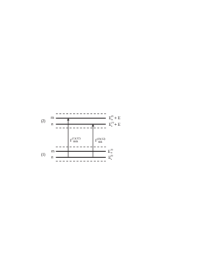
Figure 3: A TLS-quadrupole multi-level system.

It consists of two identical groups of levels (1) and (2), shifted by the TLS energy $E$. We are interested in the off-diagonal transition matrix elements $f^{(12)}_{nm}$ between these two groups of levels. In zero order ($\widehat{{\cal V}}=0$) transitions are induced by the third term in Eq. (32). However, the only non-zero off-diagonal matrix elements are the ones for transitions between identical levels in the two groups

$$f^{(0)(12)}_{nn}={\bf F}\cdot{\bf m}\frac{\Delta_{0}}{E}.$$ (33)

They are all equal and independent of $n$.

In first order of the perturbation we have also non-zero off-diagonal matrix elements for transitions between different levels in the two groups. For $n\neq m$ we have LL3

$$f^{(1)(12)}_{nm}=\underbrace{{\sum_{k\neq n}}\frac{{\cal V}_{nk}^{(11)}f_{km}^{(0)(12)}}{E_{n}^{(0)}-E_{k}^{(0)}}}_{k=m}+\underbrace{{\sum_{k\neq m}}\frac{{\cal V}_{km}^{(22)}f_{nk}^{(0)(12)}}{E_{m}^{(0)}-E_{k}^{(0)}}}_{k=n}=2\frac{{\cal V}_{nm}^{(11)}f_{mm}^{(0)(12)}}{E_{n}^{(0)}-E_{m}^{(0)}}.$$ (34)

Here we have used the property

$${\cal V}_{nm}^{(11)}=-{\cal V}_{nm}^{(22)}=-\frac{\Delta}{E}\left(\widetilde{V}_{Q}\right)_{nm},$$ (35)

which follows from the last term in Eq. (32).

The energy denominators in Eq. (34) correspond to the energy difference in one group of levels and are of the order of the small quadrupole energies $\Delta E_{Q}$. In Eq. (34) we neglected the contributions of the off-diagonal matrix elements ${\cal V}_{nm}^{(12)}$ and the diagonal matrix elements $f_{nn}^{(0)(11)}$, $f_{nn}^{(0)(22)}$. This is justified since they have much larger energy denominators, equal to the distance between two levels from two different groups. This distance is of the order of the TLS energy $E$ which is much larger than $\Delta E_{Q}$. Therefore, this contribution is small due to the small parameter $\Delta E_{Q}/E\ll 1$.

Taking into account that for real matrix $\left(\widetilde{V}_{Q}\right)_{nm}=\left(\widetilde{V}_{Q}\right)_{mn}$, we get from Eq. (34) an important relation for the off-diagonal matrix elements with $n\neq m$

$$f^{(1)(12)}_{nm}=-f^{(1)(12)}_{mn}.$$ (36)

It is equivalent to the important property that $\alpha^{(12)}_{ij}=-\alpha^{(12)}_{ji}$ for $i\neq j$.

In the second order in the perturbation we have also corrections to the off-diagonal transitions matrix elements $f^{(12)}_{nn}$ for transitions between equal levels in the two groups. Using second order perturbation theory LL3 we get after rather cumbersome calculations

$$f^{(12)}_{nn}=f^{(0)(12)}_{nn}\left[1-2\sum_{m\neq n}\left(\frac{{\cal V}^{(11)}_{nm}}{E_{n}^{(0)}-E_{m}^{(0)}}\right)^{2}\right].$$ (37)

In this approximation the matrix elements $f^{(12)}_{nn}$ differ for different $n$ and are smaller than the unperturbed values (33).

V ECHO OSCILLATIONS IN A MAGNETIC FIELD

In this section, using the above results, we will investigate the echo amplitude as a function of the time delay $\tau_{21}$ between the two electric pulses. This dependence straightforwardly give rise to the echo oscillations in the external magnetic field. For ease of understanding, let us start from the simplest case of a four-level system. This corresponds to a nuclear spin $J=1/2$ in a magnetic field. Such nuclei have zero quadrupole moment and, therefore, do not interact with a TLS. Nevertheless, formally we can consider this case to illustrate qualitatively the main features of our theory. We show that these features will be conserved in the more realistic case of $J>1/2$.

V.1 Four-Level System

In the case of $J=1/2$ we have the four-level system shown in Fig. 4.

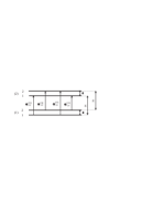
Figure 4: A four-level system for nuclear spin $J=1/2$.

Introducing the following notations for the off-diagonal matrix elements $\alpha_{ik}^{(12)}$ between two group of levels (1) and (2)

$$\alpha_{11}^{(12)}=\alpha_{22}^{(12)}=a_{0}(1-2b^{2})\equiv a,\quad\alpha_{12}^{(12)}=-\alpha_{21}^{(12)}=2a_{0}b,$$ (38)

where

$$a_{0}\equiv{\bf e}\cdot{\bf m}\,\frac{\Delta_{0}}{E},\quad b\equiv\frac{\Delta}{E}\frac{\left(\widetilde{V}_{Q}\right)_{12}}{\varepsilon},$$ (39)

and taking into account that in the framework of the perturbation theory $b\ll 1$, we get from Eq. (15) the following expression for the echo-amplitude from a four-level system

$$P_{\rm echo}=C\,\left[\left|a^{2}+4a_{0}^{2}b^{2}e^{i\varepsilon\tau_{21}}\right|^{2}+4a_{0}^{4}b^{2}\cos\varepsilon\tau_{21}\left|1-e^{i\varepsilon\tau_{21}}\right|^{2}\right]=C\,a_{0}^{4}\left(1-32b^{2}\sin^{4}\frac{\displaystyle\varepsilon\tau_{21}}{\displaystyle 2}\right)+O(b^{4}).$$ (40)

Here the coefficient $C$ includes all those factors which are for the time being irrelevant.

From Eq. (40) we can see that the echo amplitude oscillates as a function of the time delay between the two pulses, $\tau_{21}$. The frequency of these oscillations is determined by the interlevel splitting $\varepsilon$ between the levels 1 and 2. Since this splitting is a function of applied magnetic field the echo will experience oscillations when magnetic field changes.

The average level of these oscillations is given by

$$\overline{P}_{\rm echo}=C\,a_{0}^{4}(1-12b^{2}).$$ (41)

For sufficiently high magnetic fields, the interlevel splitting $\varepsilon\propto H$ and therefore, according to Eq. (39), $b\propto 1/H\to 0$ for $H\to\infty$. This means that with increasing magnetic field the average echo amplitude increases and finally approaches the value of the TLS echo amplitude, $Ca_{0}^{4}$ without a nuclear quadrupole moment. It looks as if a sufficiently high magnetic field switched off the TLS-quadrupole interaction. According to Eq. (40) we have the same value of the echo amplitude $Ca_{0}^{4}$ in the limit $\tau_{21}\to 0$ but in a final magnetic field.

V.2 TLS-Quadrupole Multi-Level System

In this section we will generalize our results to the case of an arbitrary TLS-quadrupole multi-level system. Using a notation similar to Eqs. (38) and (39)

$$\alpha_{nn}^{(12)}=a_{0}\left(1-2\sum_{m\neq n}b^{2}_{nm}\right),\quad\alpha_{nm}^{(12)}=-\alpha_{mn}^{(12)}=2a_{0}b_{nm}$$ (42)

where

$$b_{nm}=\frac{\Delta}{E}\,\frac{\left(\widetilde{V}_{Q}\right)_{nm}}{\varepsilon_{mn}},$$ (43)

and $\varepsilon_{mn}=E_{m}^{(0)}-E_{n}^{(0)}$ is the distance between the quadrupole levels (inside one level group!), we get for the echo amplitude

$$P_{\rm echo}=C\,a_{0}^{4}\left(1-\frac{64}{N}\sum_{n,m>n}b_{nm}^{2}\sin^{4}\frac{\varepsilon_{nm}\tau_{21}}{2}\right).$$ (44)

Here $N=2J+1$ and the factor C, as before, includes all irrelevant details. The average (over $\tau_{21}$) of the echo amplitude is given by

$$\overline{P}_{\rm echo}=C\,a_{0}^{4}\left(1-\frac{24}{N}\sum_{n,m>n}b^{2}_{nm}\right).$$ (45)

The quadrupole level splittings $\varepsilon_{mn}$ are functions of the external magnetic field ${\bf H}$. In the absence of any level degeneracy, in small magnetic fields when the Zeeman energy $\mu H\ll\Delta E_{Q}$, these splittings acquire a small quadratic corrections of the order of $(\mu H)^{2}/\Delta E_{Q}$. Therefore, in this case the echo amplitude attains, as a function of the applied magnetic field, oscillations with a frequency of the order of $\mu^{2}H\tau_{21}/\hbar\Delta E_{Q}$. In the case of a level degeneracy at zero magnetic field, the splittings of the originally degenerate levels are of the order $\mu H$ and, therefore, the frequency of the echo oscillations is of the order of $\mu\tau_{21}/\hbar$. A simple estimate shows that the order of the magnitude of the period of these oscillations is in a full agreement with the experimental data LESH ; LNHE .

With a further increase of the magnetic field, the Zeeman energy, $\mu H$, becomes of the order of or bigger than the typical quadrupole energy splitting $\Delta E_{Q}$ in zero magnetic field. In such magnetic fields the typical level splittings $\varepsilon_{nm}$ are mainly determined by the Zeeman energy $\mu H$ and in the limit $\mu H\gg\Delta E_{Q}$ they become linear functions of $H$. Therefore, in this case the matrix elements $b_{nm}\propto 1/\varepsilon_{nm}\propto 1/H$ are dying-off with increasing magnetic field. As a result the average echo amplitude increases, approaching for $H\to\infty$ the level of the TLS echo amplitude with zero quadrupole moment.

Above we have considered the case of one nucleus interacting with a TLS. However it can happen in glasses that many nuclei participate in a tunneling motion. In such a case, since the magnetic interaction between the nuclei can be neglected, we can easily take this into account by including in Eq. (44) a summation over the nuclei

$$P_{\rm echo}=C\,a_{0}^{4}\left(1-\sum_{s}\frac{64}{N_{s}}\sum_{n,m>n}(b_{nm}^{s})^{2}\sin^{4}\frac{\varepsilon_{nm}^{s}\tau_{21}}{2}\right),$$ (46)

where $N_{s}=2J_{s}+1$. For distant nuclei the matrix elements $b^{s}_{nm}$ depend on the distance, $R_{s}$, between the nucleus and the TLS as $b^{s}_{nm}\propto 1/R_{s}^{3}$. Therefore, the main contributions to the sum over nuclei in Eq. (46) are from nuclei participating in the tunneling and nearest neighbors.

V.3 Difference Between Integer And Half-Integer Spins

Up to now we did not discriminate between the two cases of integer and half-integer nuclear spin $J$. There is, however, an important difference between their quadrupole energy level spectra in zero magnetic field. In the case of an integer spin, $J=1,2,...$, the energy levels of the quadrupole Hamiltonian $\widehat{W}_{Q}$ (or $\widehat{\widetilde{W}}_{Q}$) in an electric field gradient tensor $\varphi_{ik}(0)$ of arbitrary symmetry are not degenerate, whereas in the case of a half-integer spin, $J=3/2,5/2,...$, according to Kramer’s theorem all energy levels of the quadrupole Hamiltonian $\widehat{W}_{Q}$ are double degenerate. This degeneracy can only be lifted by applying a magnetic field.

To calculate the echo amplitude we have used a perturbation approach for a non-degenerate case. Strictly speaking this approach is only valid in a finite magnetic field. Therefore, we now discuss the special case of a half-integer nuclear spin and $H=0$. num In this case the energy denominators of matrix elements $f_{nm}^{(1)(12)}$ and $b_{nm}$ (Eqs. (34) and (43)) are zero if $n$ and $m$ belong to a pair of Kramer’s degenerate levels. On the other hand the matrix elements $\left(\widetilde{V}_{Q}\right)_{nm}$ are also zero in this case. The reason for this is obvious. If the matrix elements were not zero the perturbation $\widehat{V}_{Q}$ (or $\widehat{\widetilde{V}}_{Q}$) would lift the Kramer’s degeneracy of the nuclear spin levels given by $\widehat{W}_{Q}$. But this cannot be the case since the interaction of the quadrupole moment with a TLS motion $\widehat{V}_{Q}$ belongs to the same symmetry class as $\widehat{W}_{Q}$. Therefore, the matrix elements belonging to a pair of Kramer’s degenerated levels $n$ and $n^{\prime}$ for $H=0$ one has for $H=0$ obey the relations

$$\left(\widehat{\widetilde{V}}_{Q}^{(0)}\right)_{nn^{\prime}}=0\quad\mbox{for}\quad n\neq n^{\prime},\quad\mbox{and}\quad\left(\widehat{\widetilde{V}}_{Q}^{(0)}\right)_{nn}=\left(\widehat{\widetilde{V}}_{Q}^{(0)}\right)_{n^{\prime}n^{\prime}}.$$ (47)

As a result, we have in our equation for half-integer spin and $H=0$ an indeterminate form $0/0$ which should be properly evaluated. For this we need the limiting behavior of both, numerator and the denominator, as $H\to 0$. It is clear that in a general the denominator, being the energy splitting between two Kramer’s levels in a magnetic field, vanishes proportional to $H$. The same is true also for the numerator. The analysis, based on a perturbation theory for degenerate levels LL3 gives the following expression for non-diagonal matrix elements describing the transition between two Kramer’s degenerate levels, $n,n^{\prime}$, split in an arbitrarily small magnetic field ${\bf H}$

$$\left(\widetilde{V}_{Q}^{(1)}\right)_{nn^{\prime}}=\sum_{m\neq n,n^{\prime}}\frac{\left({\cal H}_{H}\right)_{nm}\left(\widetilde{V}^{(0)}_{Q}\right)_{mn^{\prime}}+\left(\widetilde{V}^{(0)}_{Q}\right)_{nm}\left({\cal H}_{H}\right)_{mn^{\prime}}}{E_{n}^{(0)}-E_{m}^{(0)}}.$$ (48)

Here the superscripts $(0)$ and $(1)$ refer to the matrix elements in zero and non-zero small magnetic fields ${\bf H}$, respectively. $\left({\cal H}_{H}\right)_{nm}$ are the matrix elements of the Zeeman term, Eq. (18).

We see from Eq. (48) that the matrix elements $\left(\widetilde{V}_{Q}^{(1)}\right)_{nn^{\prime}}$ are indeed proportional to the magnetic field $H$ at small fields. Therefore, we come to the important conclusion that at zero magnetic field the ratio $\left(\widetilde{V}_{Q}^{(1)}\right)_{nn^{\prime}}/\varepsilon_{nn^{\prime}}$ has a finite value which depends on the orientation of the magnetic field ${\bf H}$ relative to the principal axes of the internal electric field gradient tensor $\varphi_{ik}(0)$. Thus, for $H=0$, the coefficients $b_{nn^{\prime}}$ for the transitions between Kramer’s degenerate levels are also finite and depend on the orientation of the applied magnetic field ${\bf H}$. In other words, we find in this case a non-analytical behavior of the functions $b_{nn^{\prime}}({\bf H})$ at ${\bf H}\to 0$.

This behavior, for half-integer spin, of the matrix elements $b_{nn^{\prime}}$ in a weak magnetic fields has important consequences. For small magnetic fields, when the Zeeman energy $\mu H$ is much smaller than the quadrupole energy $\Delta E_{Q}$, the distance between the split originally degenerate levels is of the order of $\mu H\ll\Delta E_{Q}$. On the other hand the distance between other (non-degenerate) levels is of the order of $\Delta E_{Q}$. According to Eq. (44) a contribution to the echo signal from a transition $n\to m$ is proportional to the oscillating function $(-b^{2}_{nm})\sin^{4}(\varepsilon_{nm}\tau_{21}/2)$. This function has a maximum for $\varepsilon_{nm}=0$. Therefore, for small magnetic fields, the contributions of all quasi-degenerate pairs of levels are in phase and proportional to $-\sin^{4}(\mu H\tau_{21}/2)$. With increasing magnetic field this function decreases from the value $0$ to the minimum value -1 for $\mu H\tau_{21}=\pi$. In our view, this explains why in experiment there is often a sharp maximum in the echo amplitude at zero magnetic field LESH ; LNHE . We believe that this maximum is a contribution from Kramer’s degenerate pairs of levels split by weak magnetic fields and indicates the presence of nuclei with a half-integer spin $J$ in the glass.

VI FINAL REMARKS

In this final section we address shortly the main approximations we have made and the limitations of the presented theory. As already mentioned in the beginning of the paper we have skipped in our equations all resonance factors like (5) or (6). This is possible when all such factors are similar for all transitions between two group of levels. For this, the spectral width $\hbar/\tau_{i}$ of the electric pulses should be much larger than the typical quadrupole energy splitting $\Delta E_{Q}$ which means that the electric pulses should be sufficiently short, $\Delta E_{Q}\tau_{i}/\hbar\ll 1$. Otherwise the important property $\alpha^{(12)}_{ij}=-\alpha^{(12)}_{ji}$ for $i\neq j$ which we used in the paper is not sufficient. The reason is that $i\to j$ and $j\to i$ transitions correspond to different energy differences (see Fig. 4 for example) and one therefore should multiply $\alpha^{(12)}_{ij}$ and $\alpha^{(12)}_{ji}$ with different resonance factors $\beta_{ij}$. In such a case the final expression for the echo amplitude becomes much more cumbersome.

The other approximation we made was that we considered the limit of a rather small electric field amplitudes when the Rabi frequencies $({\bf F}_{1,2}\cdot{\bf m})\,\Delta_{0}/\hbar E$ are much smaller than $\hbar/\tau_{i}$. In the case of short electric pulses (as was indicated above) this limitation can be easily overcome and one can show that Eq. (44) for the echo amplitude will remain valid and only the coefficient $C$ changes.

References

- (1) S. Ludwig, C. Enss, P. Strehlow, and S. Hunklinger, Phys. Rev. Lett. 88, 075501 (2002).
- (2) S. Ludwig, P. Nagel, S. Hunklinger, and C. Enss, J. Low-Temp. Phys. 131, 89 (2003).
- (3) C. Enss, and S. Ludwig, Phys. Rev. Lett 89, 075501 (2002).
- (4) A. Wüger, A. Fleischmann, and C. Enss, Phys. Rev. Lett. 89, 237601 (2002).
- (5) V. L. Gurevich, M. I. Muradov, and D. A. Parshin, Europhys. Lett. 12, 375 (1990).
- (6) V. L. Gurevich, M. I. Muradov, and D. A. Parshin, Sov. Phys. JETP 5, 928 (1990).
- (7) Please note that the full and the dashed line should start from the same level (point on Fig. 2). Otherwise an additional exponential factor is present. It shows the random initial phase difference between the levels and averages to zero.
- (8) A. Abragam, The Principles of Nuclear Magnetism, p. 163, Oxford 1961.
- (9) D. A. Parshin, Sov. Phys. Solid. State, 36, 991 (1994).
- (10) L. D. Landau and E. M. Lifshitz, Quantum Mechanics: Non-relativistic theory, Third Edition, 1981.
- (11) For numerical calculations this problem is of no importance since for any small but finite value of the magnetic field our equations are valid.