Modelling one-dimensional driven diffusive systems by the Zero-Range Process

Abstract

The recently introduced correspondence between one-dimensional two-species driven models and the Zero-Range Process is extended to study the case where the densities of the two species need not be equal. The correspondence is formulated through the length dependence of the current emitted from a particle domain. A direct numerical method for evaluating this current is introduced, and used to test the assumptions underlying this approach. In addition, a model for isolated domain dynamics is introduced, which provides a simple way to calculate the current also for the non-equal density case. This approach is demonstrated and applied to a particular two-species model, where a phase separation transition line is calculated.

I Introduction

Phase separation in one-dimensional driven systems has attracted much attention of late Zia ; Mukamel00 ; Evans00 ; Schutz03 . In contrast to equilibrium one-dimensional systems, where phase separation cannot occur unless the interactions are long ranged, several examples of phase transitions in one-dimensional non-equilibrium steady states have been given Evans98 ; LBR00 ; Rittenberg99 ; RSS ; Kafri02A ; Kafri03 ; CDE . These models generally have local noisy dynamics and some conserved quantity or quantities driven through the system. Particular attention has been paid to a simple yet general class of models with two species of particles which are conserved under the dynamics Zia ; Schutz03 . These models are defined on a ring, where each site can take one of three states: vacant, occupied by a positive particle, or occupied by a negative particle. Two conservation laws are obeyed by the dynamics, which can be cast into two conserved quantities – the total density of particles in the system, $\rho$, and the fraction $\eta$ of positive particles out of the total number of particles. To study these models a coarse-grained description has been developed Kafri02A . In this description one views the microscopic configuration of the model as a sequence of particle domains, bounded by vacancies. Each domain is defined as a stretch of particles of both types. The idea is to view particle domains as urns which may exchange particles. At a coarse-grained level one identifies the current of particles through a domain as the hopping rate of particles between neighbouring urns (see Fig. 1). This coarse-grained description then defines a Zero-Range Process (ZRP) for which the steady state may be solved exactly. When such correspondence is applicable one can use the ZRP to obtain the distribution of the domain size, although information about the correlation between the two species of particles is lost. Generally the identification of the driven system with a ZRP is at a coarse-grained level and is not exact. Rather, it relies on the applicability of some physical assumptions, as discussed below. However, for a particular model for which an exact solution of the steady state exists, it could be shown that the mapping of the steady state to that of a ZRP is indeed exact Kafri02A . The correspondence between driven models and the ZRP may be used to address the question of existence of phase separation in the driven model Kafri02A . In such a transition a fluid phase, where the distribution of particles and vacancies is homogeneous, becomes upon increasing $\rho$ a phase separated state. This state is characterized by macroscopic particle domain devoid of vacancies. In the context of the ZRP the transition into the phase separated state corresponds to a condensation transition whereby one urn becomes filled by a macroscopic number of particles OEC ; Evans00 .

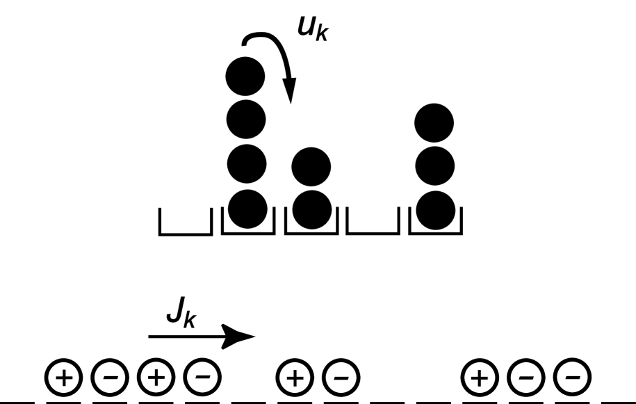
Figure 1: A microscopic configuration of a two-species driven model (bottom) and its corresponding configuration in the ZRP (top).

A careful analysis of the corresponding ZRP suggested the following criterion for phase separation. Let $u_{k}$ be the rate at which particles leave a domain of size $k$. If $u_{k}$ vanishes in the thermodynamic limit $k\to\infty$, phase separation is expected at any density. Otherwise, for large domains, $u_{k}$ typically takes the form

$$u_{k}=u_{\infty}\left(1+\frac{b}{k}\right)\;,$$ (1)

where $u_{\infty}$ and $b$ are constants. The existence of phase separation is then related to the value of $b$. Phase separation cannot exist as long as $b\leq 2$. However, if $b>2$ a phase transition into a phase separated state occurs as the particle density is increased. This picture has been used to argue against the existence of phase separation in some models Kafri02A , to study crossover phenomena Kafri02B , and to suggest a model which does exhibit a phase transition into a phase separated state Kafri03 . In order to apply the ZRP picture for a given model one has to evaluate the rates $u_{k}$ by which domains exchange particles. This may be too difficult a task to carry out analytically, and may involve exceedingly large computation time to estimate numerically. However, it has been suggested that in order to estimate $u_{k}$ one may reduce the full many-domain system into a single isolated domain problem. This is done by modelling an isolated domain by an open chain of particles exchanging particles with reservoirs at its ends. At the boundaries, particles are injected and ejected at constant rates. When these rates are large enough, the system is known to be forced into a maximal-current phase with a bulk density $\eta=1/2$ Krug91 . This approach is therefore only applicable when the densities of the two species of particles in the full model are equal, and each domain is stationary on average. In this case the rate $u_{k}$ is directly related to the current $J_{k}$ which flows through the domain. Thus, for equal densities of positive and negative particles the many-domain problem is simplified to the problem of a single domain of fixed size. The calculation of the current through the single domain may be tackled numerically or analytically, when possible Kafri02A ; Kafri03 . It is important to notice that the approach outlined above for describing a many domain system by a ZRP relies on two assumptions. Firstly, it is assumed that domains are uncorrelated, in the sense that the current $J_{k}$ flowing through a given domain depends only on its own size. Secondly, the current through a domain of length $k$ is assumed to take its steady state value with respect to a system of size $k$ (even though $k$ fluctuates) and this steady state value is identified with that of an open system. In this paper we seek to test these underlying assumptions. Whereas in previous studies the current $J_{k}$ of a domain of length $k$ was studied using an isolated single domain, here we introduce a numerical method for directly measuring $J_{k}$ of a fluctuating domain within the full system. An agreement between the two methods validates the assumptions behind the criterion. We also seek to extend the approach to treat the case of non-equal densities. As discussed above, modelling a single domain by an open system is not applicable in this case. Moreover since we have unequal densities of positive and negative particles, the vacancies are not stationary and drift on average. Thus in order to reduce the many-domain problem to a single domain problem we have to deduce the appropriate ensemble for the single domain. In this paper we propose a model for a fluctuating isolated single domain which can be used to calculate a steady state current $J_{k}$ in a domain of non-equal densities. This result is checked by using the direct measurement discussed in the previous paragraph. Moreoever in a limiting case we can solve the model exactly through a matrix product ansatz and show that it produces the correct ensemble. This paper is organized as follows. In Section 2 we define a specific model that we use to demonstrate our approach. In Section 3 we describe the method for direct measurement of the currents within the many-domain system, and apply it to both cases of equal and non-equal densities. A model for an isolated domain which is not restricted to the case of equal densities is introduced in Section 4 and an exact solution of a limiting case is given. We then discuss generalizations of the approach to other models in Section 5, and present a summary and outlook in Section 6.

II Model definition and some known results

In order to study the correspondence between driven diffusive systems and the ZRP, we consider in the main body of this paper a particular driven model as a test case. In this section we define the model and present some analytical results. The model is defined on a one-dimensional ring of $L$ sites. Each site $i$ is associated with a ‘spin’ variable $s_{i}$. A site can either be vacant ($s_{i}=0$) or occupied by a positive ($s_{i}=+1$) or a negative ($s_{i}=-1$) particle. Particles are subject to hard-core repulsion and a nearest-neighbor ‘ferromagnetic’ interaction, defined by the potential

$$V=-\frac{\epsilon}{4}\sum_{i}s_{i}s_{i+1}\;.$$ (2)

Here $0\leq\epsilon<1$ is the interaction strength, and the summation runs over all lattice sites. The model evolves according to the nearest-neighbour exchange rates

$$+-\mathop{\longrightarrow}^{1+{\rm\Delta}V}-+\hskip 19.91684pt+0\mathop{\longrightarrow}^{\alpha}0+\hskip 19.91684pt0-\mathop{\longrightarrow}^{\alpha}-0\;,$$ (3)

where ${\rm\Delta}V$ is the difference in the potential $V$ between the initial and final states. The number of particles of each species, $N_{+}$ and $N_{-}$, are conserved by the dynamics. Alternatively, the system can be characterized by two conserved densities, namely the total density $\rho=(N_{+}+N_{-})/L$, and the relative density $\eta=N_{+}/(N_{+}+N_{-})$ . This model, which is a generalization of the Katz-Lebowitz-Spohn model KLS ; Hager01 , was introduced in Kafri03 and studied for the case of equal densities of positive and negative particles, $\eta=1/2$.

II.1 The non-interacting case, $\epsilon=0$

Let us first discuss the case $\epsilon=0$, where particles only interact through the hard-core exclusion. In this case an exact solution shows that within a grand-canonical ensemble to be defined below domains are uncorrelated, and the steady-state weight factorizes into a product of single-domain terms. This is the case for both equal and non-equal densities of the two species. These results are obtained by considering a grand-canonical ensemble in which the number of vacancies $M$ is kept constant. The number of particles of each species, and thus the size of the lattice, are allowed to fluctuate. A fugacity $\xi$ is attached to the positive particles, thus controlling the relative density between the two species ($\xi=1$ corresponds to equal densities). All configurations of the system can be described in terms of domains of particles, where a domain is defined as an uninterrupted sequence of particles of both species. The weight $W_{M}(\{k_{i}\})$ of all configurations in which $k_{i}$ particles reside in the $i$th domain is then given by

$$W_{M}(\{k_{i}\})=\prod_{i=1}^{M}{z^{k_{i}}Z_{k_{i}}(\xi)}\;,$$ (4)

where $Z_{k}$ is the sum over all weights of microscopic configurations of a domain of length $k$, and $z$ is the fugacity, which controls the overall density of particles in the system. Hence, within the grand canonical ensemble domains are statistically independent with a domain size distribution

$$P(k)\sim z^{k}Z_{k}(\xi)\;.$$ (5)

The grand canonical partition function is given by

$${\cal Z}_{M}=\sum_{\{k_{i}\}}\prod_{i=1}^{M}{z^{k_{i}}Z_{k_{i}}(\xi)}\;.$$ (6)

In the equal density case the exact solution reveals that $Z_{k}$ is identical to the partition function of the totally asymmetric exclusion process on a one-dimensional lattice of $k$ sites with open boundary conditions Derrida93 . For non-equal densities, it turns out that $Z_{k}$ is identical to the grand-canonical partition function of the same process defined on a ring of size $k+1$ with a single vacancy Mallick96 ; Sasamoto00 . In both cases

$$Z_{k}\sim(1+\sqrt{\xi})^{2k}/k^{3/2}$$ (7)

for large $k$. The resulting distribution function (5) implies that the model does not exhibit phase separation at any density. In particular, for any choice of $\rho$ one can choose the fugacity $z<1$ such that the average density satisfies $\rho/(1-\rho)=\int kP(k)dk$. Moreover, in the case $\epsilon=0$ the correspondence between the steady-state of the model and that of the ZRP can be made explicit. Within a grand-canonical ensemble of the ZRP urns are statistically independent. The distribution function $P_{\mbox{\tiny ZRP}}(k)$ for the occupation of a single urn is given by $P_{\mbox{\tiny ZRP}}(k)\sim z^{k}\prod_{m=1}^{k}1/u_{m}$. On the other hand, in the $\epsilon=0$ driven model the steady-state current $J_{k}$ flowing through a domain is given by $J_{k}=Z_{k-1}/Z_{k}$. The steady-state distribution function (5) can then be written as $P(k)\sim z^{k}\prod_{m=1}^{k}1/J_{m}$. Thus $P(k)=P_{\mbox{\tiny ZRP}}(k)$ with $u_{k}=J_{k}$. Using (7) one obtains $b=3/2$ for this case, implying no phase separation.

II.2 The interacting case, $\epsilon>0$, at $\eta=1/2$

We now turn to the more general case, $\epsilon\neq 0$. Here no exact mapping to the ZRP is available. However, it was conjectured in Kafri02A ; Kafri03 that the physical picture obtained for the non-interacting case remains valid, namely that the hopping rates of a corresponding ZRP should be identified as the steady-state currents of isolated domains. One therefore needs to calculate the asymptotic form of the steady-state current running through a domain, $J_{k}(\epsilon)\sim J_{\infty}(\epsilon)\left(1+b(\epsilon)/k\right)$. For $\eta=1/2$, where the average domain velocity vanishes, the current $J_{k}$ may be calculated by considering an isolated domain with open boundaries, which exchanges particles with reservoirs at its ends at high rates. It has been argued Krug90 ; Krug97 that the coefficient $b(\epsilon)$ of an isolated open domain is given by

$$b(\epsilon)=c\;b_{R}(\epsilon,\eta=1/2)\;.$$ (8)

Here $b_{R}(\epsilon,\eta)$ is the coefficient corresponding to a closed fully-occupied ring, and $c$ is a universal constant which is equal to $3/2$. For a ring the coefficient $b_{R}(\epsilon,\eta)$ can be calculated at any density $\eta$ Kafri03 . It is given by

$$b_{R}(\epsilon,\eta)=-\frac{\lambda(\epsilon,\eta)\kappa(\epsilon,\eta)}{2J_{\infty}(\epsilon,\eta)}\;.$$ (9)

In this expression $\lambda=\partial^{2}J^{R}_{\infty}/\partial\eta^{2}$. The compressibility $\kappa=\lim_{k\to\infty}k^{-1}\left(\langle\eta^{2}\rangle-\langle\eta\rangle^{2}\right)$ is evaluated in a grand-canonical ensemble of a fully-occupied ring with average density $\langle\eta\rangle=1/2$. Using the known properties of the steady state of this model KLS ; Hager01 it can be shown that

$$J^{R}_{\infty}(\epsilon,\eta) = \left[\gamma+\epsilon\sqrt{4\eta(1-\eta)}\right]\gamma^{-3}$$ (10)

$$\kappa(\epsilon,\eta) = \eta\left(1-\eta\right)\sqrt{1+4\eta\left(1-\eta\right)\left({\frac{1+\epsilon}{1-\epsilon}}-1\right)}$$ (11)

where $\gamma=[4\eta\left(1-\eta\right)]^{-1/2}+[(4\eta(1-\eta))^{-1}-1+(1+\epsilon)/(1-\epsilon)]^{1/2}$. Inserting (10) and (11) into (9) with $\eta=1/2$ one obtains the coefficient $b$ of an open domain as a function of $\epsilon$ for the equal density case. It is found that $b>2$ for $\epsilon>4/5$. The criterion mentioned above therefore implies that in this model phase separation takes place at high density $\rho$ for any $\epsilon>4/5$. Note that although the expression of $b_{R}(\epsilon,\eta)$ is valid for arbitrary $\eta$ in the ring geometry, the resulting $b(\epsilon)$ (Eq. 8) is relevant to a domain with open boundaries only at $\eta=1/2$. A single domain model which is applicable for $\eta\neq 1/2$ will be discussed in Section IV.

Figure 2: Density profile of a domain of size $k=100$ at equal densities ($\eta=1/2$) and $\epsilon=1/2$. Solid line corresponds to direct simulation of the full many-domain model. Plus signs correspond to an open isolated domain, and squares correspond to the non-conserving single-vacancy ensemble.

III Direct numerical measurement of domain dynamics

We now describe our method for a direct numerical measurement of the flow of particles $u_{k}$ out of a domain of size $k$. As discussed in the introduction, this method involves the full many domain system, and thus allows a check on the validity of reducing to the problem to that of a single domain. The idea is during a simulation of duration $T$ to record the number of hopping events out of a domain of size $k$, and the average number of domains of size $k$. The ratio of these quantities yields $u_{k}$. Here one unit of time corresponds to a single Monte-Carlo sweep. We thus define

$$N_{k}=\frac{1}{T}\sum_{t=t_{0}}^{t_{0}+T}m_{k}(t)\hskip 19.91684ptF_{k}=\frac{1}{T}\sum_{t=t_{0}}^{t_{0}+T}f_{k}(t)\;.$$ (12)

Here $m_{k}$ is the number of domains of size $k$ residing in the system at time $t$, and $f_{k}(t)$ is the number of exchanges $+0\to 0+$ occurred between times $t$ and $t+1$ at the boundaries of domains of size $k$. Of course, one can also define $f_{k}$ through the transition rates $0-\to-0$, without changing the following discussion. The measurement starts at time $t_{0}$, after short-time relaxations are over. Clearly,

$$u_{k}=\lim_{T\to\infty}\frac{F_{k}}{N_{k}}\;.$$ (13)

In practice, the measurement time $T$ taken to be large enough to ensure convergence. Estimates for $u_{\infty}$ and $b$ are then obtained from the linear fit of $u_{k}$ to $1/k$. However one can exploit the data obtained from numerical simulations better by integrating the distributions. Thus we define

$$\widetilde{N_{k}}=\sum_{\ell=k}^{\infty}N_{\ell}~{}~{}~{}\widetilde{F_{k}}=\sum_{\ell=k}^{\infty}F_{\ell}~{}~{}~{}\widetilde{Q_{k}}=\widetilde{N_{k}}^{-1}\sum_{\ell=k}^{\infty}\frac{N_{\ell}}{\ell}\;.$$

Using $u_{k}=u_{\infty}(1+b/k)$ one has

$$\tilde{u}_{k}=\frac{\widetilde{F_{k}}}{\widetilde{N_{k}}}=u_{\infty}\left(1+b\widetilde{Q_{k}}\right)$$ (14)

and one obtains $b$ and $u_{\infty}$ from a linear fit.

III.1 Equal densities, $\eta=1/2$

While simulating the dynamics of the full model we have recorded the density profiles of domains of a give size $k$. These profiles are compared with those obtained from the single open domain calculation in Fig. 2. Both profiles are identical to within the statistical fluctuations except at sites 1 and $k$ where there are systematic deviations. The deviations at these two sites are to be expected as this is where the dynamics for the single domain is simplified from the full model. The excellent agreement between the profiles indicates that the single open domain properly models a fluctuating domain in the full system.

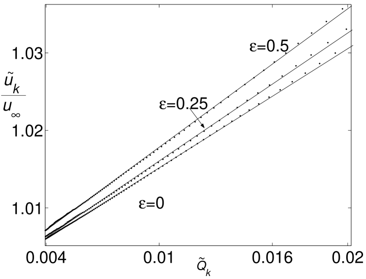
Figure 3: Results of numerical simulations of the full model for $\eta=1/2$ and $\rho=0.7$, from which $b(\epsilon)$ and $u_{\infty}$ are estimated. Solid lines are obtained by linear fits of the data.

We now apply the direct numerical method outlined above to the case $\eta=1/2$. The results of numerical simulations are given in Fig. 3 for several values of $\epsilon$. Table 1 summarizes the resulting parameters $b(\epsilon)$ and $u_{\infty}$. For $\epsilon=0$ one knows from the exact correspondence of the model to ZRP that $u_{k}=J_{k}=\frac{1}{4}\left(1+\frac{3/2}{k}\right)$. Our direct measurement of $\tilde{u}_{k}$ recovers these results quite faithfully. In general, for $\epsilon>0$ we find that the measured values of $b$ and $u_{\infty}$ are in close agreement with (8–11). Thus we conclude that the current flowing through a domain in the model can indeed be viewed as the stationary current flowing trough an isolated open system of the same size. The proposition that by increasing $\epsilon$ a phase transition into a phase separated state occurs is thus verified.

	$b(\epsilon)$	$b$	$u_{\infty}$	$u_{\infty}$
$\epsilon$	(Eq. 8)	measured	(Eq. 10)	measured
0	1.5	1.51	0.25	0.25
0.25	1.67	1.65	0.2113	0.2115
0.5	1.82	1.79	0.1585	0.1583
0.8	2	2.05	0.075	0.0749

Table 1: Results of direct measurement of $u_{k}$ in the full model, compared with analytical results of Section 2. We estimate the error in the measurement of $u_{\infty}$ to be $0.0005$ and of $b$ to be $0.05$.

III.2 Non-equal densities, $\eta\neq 1/2$

We now consider the model with non-equal densities of the two particle species, $\eta\neq 1/2$. In order to apply the criterion for phase separation one needs to calculate the coefficient $b(\epsilon,\eta)$. As mentioned in Section II, an exact mapping to the ZRP is only available at $\epsilon=0$, where one finds $b=3/2$ for any value of $\eta$. To test the validity of the correspondence to ZRP and evaluate $b(\epsilon,\eta)$ for $\epsilon\neq 0$ and arbitrary $\eta$ one has to resort to direct numerical simulations, as discussed above. We have simulated the model for $\epsilon=0.25,0.5$ and $\eta=0.6,0.75,0.85$. The values of $b$ are extracted from the outflow of particles of domains of size up to $250$. We note that we could obtain an accurate estimate for $b$ in this way only for the outflow of the majority species. Getting similar estimates for the minority species would require significant statistics for much larger domains.

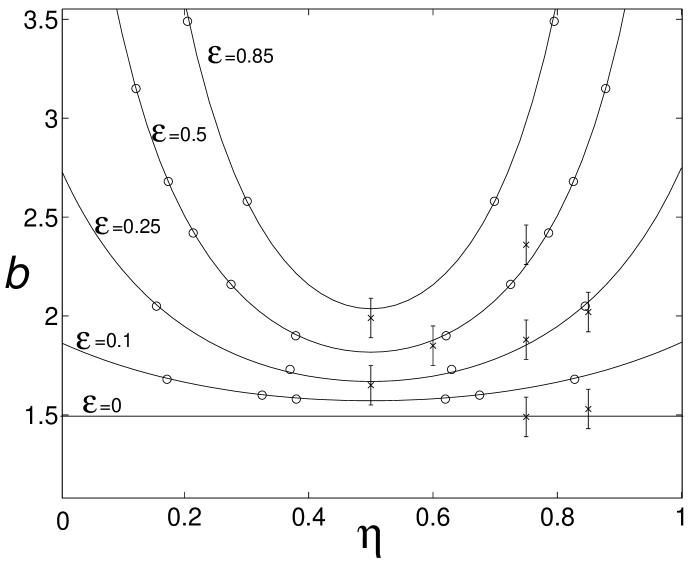
Figure 4: The coefficient $b$ as a function of the density $\eta$ of positive particles within a domain. Solid lines are given by (8), crosses are direct measurements in the full system, while circles correspond to the non-conserving vacancy ensemble.

In Fig. 4 we display the values of $b$, as obtained from direct measurement of the outflow of majority particles. Although a priory one does not expect $b(\epsilon,\eta)$ to be given by the expression obtained from the ring model of Section II.2, $b(\epsilon,\eta)=3/2\;b_{R}(\epsilon,\eta)$, we also display in this figure the expression obtained from this formula. We find that the numerical data agrees very well with these curves. This suggests that in fact the analytical results obtained from the ring model (8–11) are valid for non-equal densities ($\eta\neq 1/2$) as well.

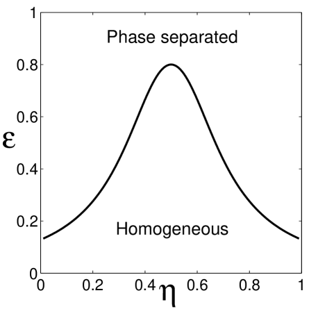
Figure 5: Phase diagram for the model, as obtained by setting $b=2$ in Eq. 8.

We conclude that $b(\epsilon,\eta)=3/2\;b_{R}(\epsilon,\eta)$, where $b_{R}(\epsilon,\eta)$ is given by (9), provides the correct expression for $b(\epsilon,\eta)$ for the full model. According to the criterion discussed in the introduction, a phase transition into a phase separated state is expected at some critical density $\rho$ for $b>2$. The transition line in the $(\epsilon,\eta)$ plane between the homogeneous and the phase separated state is depicted in Fig. 5. For values of $\epsilon$ which are larger than $0.8$ phase separation is expected at high densities for any value of $\eta$. On the other hand, for $\epsilon\lesssim 0.129$ phase separation does not occur at any density. Direct numerical observation of the predicted transition line is hard to obtain. For $\eta$ not too close to $1/2$ one would need to simulate exceedingly large systems, far beyond our present reach, in order for the fluid to sustain domains which are large enough that the current flowing through them takes the asymptotic form. It thus remains a challenge to devise some method for numerical observation of this transition line.

IV Single domain with non-equal densities: non-conserving vacancy ensemble

As discussed above, for the case of equal densities of positive and negative particles one can model a domain of length $k$ as an open boundary segment of length $k$ where particles enter and exit at the boundaries. This is by virtue of the fact that for sufficiently high entry and exit rates, the open segment will be maintained in a maximal current phase where the bulk density of positive particles organises itself to be $\eta_{\rm bulk}=1/2$. One uses the ensemble of the open boundary problem to calculate the dependence of the current on domain length. The maximal current phase exhibits long-range correlations that ultimately generate a slow decay of the current with domain length and a condensation transition if $\epsilon$ is sufficiently large. However an open boundary segment cannot produce a bulk density $\eta_{\rm bulk}\neq 1/2$ and retain long-range correlations i.e. it cannot produce a maximal current phase with $\eta\neq 1/2$. Thus, for the case of non-equal densities of positive and negative particles one cannot use the ensemble generated by the open boundary problem to calculate the current for a domain of size $k$. Instead one must devise an alternative ensemble that allows the density of the domain to fluctuate about a value $\eta\neq 1/2$ whilst retaining the long-range correlations required in a maximal current phase. In this section we propose an ensemble for the single domain of length $k$ that is generated by the dynamics of a single vacancy on a ring of size $k+1$. The same dynamics as the full model is used for the exchange of particles (3). Also the dynamics of the vacancy retains the processes present in the full model

$$+\,0 \rightarrow 0\,+\;,\qquad\textrm{with rate $\beta$}\;,$$

$$0\,- \rightarrow -\,0\;,\qquad\textrm{with rate $\alpha$}\;.$$ (15)

However in addition we introduce two processes where particles are not conserved

$$+\,0 \rightarrow 0\,-\;,\qquad\textrm{with rate $\delta$}\;,$$

$$0\,- \rightarrow +\,0\;,\qquad\textrm{with rate $\gamma$}\;.$$ (16)

Note that in (15) we have generalised (3) to include a rate $\beta$. We now show that in the case $\epsilon=0$ the above dynamics generates precisely the ensemble required for a domain of length $k$. To demonstrate this we solve exactly the steady state of the non-conserving vacancy problem using a matrix product ansatz.

IV.1 Exact solution for $\epsilon=0$

The matrix product ansatz entails writing the steady state as a product of matrices Derrida93 ; DJLS i.e. the steady state weight $w(\{s_{i}\})$ for configuration $\{s_{i}\}=s_{1},\ldots,s_{k}$. is

$$w(\{s_{i}\})=\rm{Tr}[X_{1}\cdots X_{k}]\;,$$ (17)

where the matrix ${\rm X}_{i}$ is

$${\rm X}_{i}=\left\{\begin{array}[]{ll}D&\quad\textrm{if $\;s_{i}=+$}\;,\\ E&\quad\textrm{if $\;s_{i}=-$}\;,\\ A&\quad\textrm{if $\;s_{i}=0$}\;.\end{array}\right.$$

Then it can be shown following Derrida93 ; DJLS , that the steady state weights for the present model can be written in this form provided the matrices $D$, $E$ and $A$ satisfy the quadratic relations

$$DE = D+\xi E\;,$$ (18)

$$\beta DA = \xi A\;,$$ (19)

$$\alpha AE = A\;,$$ (20)

where $\xi\alpha\delta=\beta\gamma$. For the conserving case $\gamma=\delta=0$, $\xi$ is not fixed and may conveniently be set to $\xi=1$. This recovers the previously known solution DJLS ; Rittenberg99 . However, for $\gamma$, $\delta\neq 0$, we must take

$$\xi=\frac{\beta\gamma}{\alpha\delta}\;.$$ (21)

Relations (18–20) are satisfied if we take $A$ to be the projector $|V\rangle\langle W|$, where we employ a bra-ket notation to denote the left and right vectors $\langle W|$ and $|V\rangle$. Then letting $D=\xi\widetilde{D}$ relations (18–20) reduce to

$$\widetilde{D}E = \widetilde{D}+E\;,$$ (22)

$$\beta\widetilde{D}|V\rangle = |V\rangle\;,$$ (23)

$$\alpha\langle W|E = \langle W|\;.$$ (24)

Relations (22–24) obeyed by $\widetilde{D}$, $E$, $\langle W|$ and $|V\rangle$, are precisely those obeyed by the matrices and vectors used to solve the steady state of the open boundary ASEP Derrida93 . Thus the weights for the non-conserving vacancy are equal to those for an open boundary system reweighted by a factor $\xi^{N_{+}}$; $\xi$ acts as a fugacity to tune the relative density of positive and negative particles. The partition function for the non-conserving vacancy system is given by summing over all possible configurations of positive and negative particles on the ring and results in

$$Z_{k}=\mbox{Tr}\left[A(\xi\widetilde{D}+E)^{k}\right]=\langle W|(\xi\widetilde{D}+E)^{k}|V\rangle$$ (25)

which is precisely the partition function for a domain of length $k$ required in the grand canonical partition function for the full system (i.e. fixed number of vacancies, fluctuating particle numbers, see Section II (4,5,6))

$${\mathcal{Z}}_{M}=\left[\sum_{k=0}^{\infty}z^{k}Z_{k}(\xi)\right]^{M}\;.$$ (26)

Thus we have shown that in the case $\epsilon=0$ the non-conserving vacancy generates the required ensemble for domains. For $\epsilon>0$ we will provide numerical evidence that this is still the case.

IV.2 Numerical Simulations for $\epsilon>0$

We ran numerical simulations of the non-conserving vacancy system and measured the density profiles as seen from the vacancy. In Fig. 2 we compare the density profile for the non-conserving vacancy problem at $\xi=1$ (corresponding to $\langle\eta\rangle=1/2$) with the density profile of domains of the same size computed in simulations of the full model and those of an open isolated domain. Again we find the profiles identical to within the statistical fluctuations except at sites 1 and $k$. We have also compared the profiles obtained in the non-conserving vacancy ensemble at non-equal densities ($\eta=0.275$) with those obtained from the direct numerical simulations of the full model (Fig. 6). The very close agreement of the profiles in the bulk of the domains provide strong evidence that the non-conserving vacancy generates the correct ensemble for domains. To evaluate $b(\epsilon,\eta)$ we measured the decay of the current $J_{k}(\epsilon,\eta)$ with the system size $k$. As in Section III we define the current as the rate at which positive particles exchange with the vacancy. The current $J_{k}(\epsilon,\eta)$ is obtained by simulating a system of size $k+1$, fixing $\xi$ (Eq. 21) such that the average density of positive particles matches $\eta$. The coefficient $b(\epsilon,\eta)$ is then obtained by comparing the currents $J_{k}$ with the asymptotic form $J_{\infty}\left(1+b/k\right)$. This requires extensive numerical calculation since the current is measured only through the single vacancy, taken to be at site 1, and no spatial averaging takes place. To overcome this difficulty simulations were performed using a multi-spin coding technique multispin . This allows many simulations to be run in parallel utilising the same random numbers. The resulting $b(\eta)$ for various values of $\epsilon$ is given in Fig. 4. These results compare very well with the analytical results obtained from the conserving ring model of Section II.2 (Eqs. 8–11), and with the numerical results of the full model.

Figure 6: Density profile of a domain of size $k=100$ at non-equal densities $\eta=0.275$ and $\epsilon=1/2$. Solid line corresponds to direct simulation of the full many-domain model. Squares correspond to the non-conserving single-vacancy ensemble with $\xi=1/2$.

V Generalization to other models

In previous sections we focused on the model presented in Section 2. However, the direct numerical approach for calculating $b$, introduced in Section III is applicable for other models as well. This method may be used to test the assumptions behind the correspondence of a driven model to the ZRP, and the applicability of the criterion for phase separation, discussed in the introduction. Also, in cases where the correspondence between the driven model and the ZRP is exact, the question of phase separation in the driven model may be rigorously answered. As an example where the numerical method for studying domains in the full model we consider a two-lane variant of the model discussed above. It has been proposed that when the rates (3) with $\epsilon=0$ are considered in a two-lane geometry, phase separation may take place Korniss . In this case the model is defined on a lattice of size $2\times L$, with periodic boundary conditions in both directions, where particles can move either within a lane or between the lanes. Direct numerical simulations of the model suggest the existence of phase separation at equal densities of the two species. However, calculating $b$ by numerical simulations of single open domains yields $b\simeq 0.8$, indicating that phase separation does not occur in this model Kafri02A . Since no exact mapping to ZRP exists in this case, we have tested this result by carrying out direct numerical measurement of $b$ in the full model as introduced in Section III. We find that indeed $b\simeq 0.8$ also in the full model, verifying the single open domain approach in this case. Finally, consider another variant of the model of Section 2, whereby the particle exchange rate (3) is replaced by $+-\rightarrow-+$ with rate $1$ and $-+\rightarrow+-$ with rate $q$. This is a generalization of the $\epsilon=0$ case, allowing for backward hopping. This model was introduced in Rittenberg99 and studied in Rittenberg99 ; RSS ; Kafri02A ; Kafri02B for equal densities, and in Arndt02 for non-equal densities. With $q<1$ this case is qualitatively similar to the $\epsilon=0$ case considered above, with no phase separation taking place at any density. However, for $q>1$ it can be shown that the steady state weight has the same form as (4), with $Z_{k}\sim(1+\sqrt{\xi})^{k}q^{\frac{1}{4}k^{2}}$ with $\xi=1$ for equal densities Blythe00 . Since this model is exactly mapped onto a ZRP, this result may be used to demonstrate that the model exhibits phase separation at any non-vanishing densities $\rho$ and $\eta$. From the above result for $Z_{k}$ it follows that for large $k$ the current in this case is given by $J_{k}=Z_{k-1}/Z_{k}\sim q^{-k/2}$, which vanishes in the limit $k\to\infty$. Thus the criterion correctly predicts strong phase separation for all densities of positive and negative particles.

VI Summary and Discussion

In this paper the correspondence between one-dimensional two-species driven models and the Zero-Range Process is reviewed and extended to consider the case of non-equal particle densities. This is demonstrated for a two-species exclusion model with ‘ferromagnetic’ interactions. To apply this correspondence one has to evaluate the length-dependence of the current emitted from a domain of particles. Previous studies were restricted to equal densities, were the average velocities of domains is zero. In these studies domains were assumed to be statistically independent, and the current is calculated using a model of single domain with open boundaries. In the case of non-equal densities domains have a non-zero average velocity, and thus this approach is not applicable. In the present work we have introduced a method for evaluating the current of a domain of length $k$ by direct numerical simulation of the full many-domain model. In the case of equal densities this method yields the same results as before, verifying the validity of the assumptions made in formulating the correspondence to ZRP. Namely that domains are statistically independent and that the current of a domain is given by the steady state current of an isolated domain. Moreover, this method may be applied to the non-equal density case. We also introduced a model for a single domain, which enables one to calculate the current of a domain without having to resort to a simulation of the full model. Here a domain is modelled by a ring with a single vacancy, with non-conserving dynamics at the vacant site. It is demonstrated that this ensemble yields the same density profiles and the currents as domains in the full model. It thus provides a rather simple way of analyzing the full model. Furthermore, we have outlined an exact solution for the non-conserving vacancy model in the case $\epsilon=0$ which extends the range of models solved by the matrix product ansatz. The phase diagram of the model in the interaction–density $(\epsilon,\eta)$ plane has been calculated using both methods, and the transition line to the phase separated state has been found. Applications to other models have also been discussed. We thank Yariv Kafri and Francesco Ginelli for helpful discussions. This study was supported by the Israel Science Foundation (ISF). Visits of MRE to Weizmann Institute were supported by the Albert Einstein Minerva Center for Theoretical Physics.

References

- (1) B. Schmittmann and R.K.P. Zia, Statistical Mechanics of Driven Diffusive Systems, Vol. 17 of Phase Transitions and Critical Phenomena, edited by C. Domb and J. L. Lebowitz (Academic Press, 1995).
- (2) D. Mukamel in Soft and Fragile Matter: Nonequilibrium Dynamics, Metastability and Flow, edited by M.E. Cates and M.R. Evans, (Institute of Physics Publishing, Bristol, 2000).
- (3) M.R. Evans, Braz. J. Phys. 30, 42 (2000).
- (4) G.M. Schütz, J. Phys A: Math. Gen. 36, R339 (2003).
- (5) M.R. Evans, Y. Kafri, H.M. Koduvely, and D. Mukamel, Phys. Rev. Lett. 80, 425 (1998); Phys. Rev. E 58, 2764 (1998).
- (6) R. Lahiri and S. Ramaswamy, Phys. Rev. Lett. 79, 1150 (1997); R. Lahiri, M. Barma, and S. Ramaswamy, Phys. Rev. E 61 1648 (2000).
- (7) P.F. Arndt, T. Heinzel, and V. Rittenberg, J. Phys A: Math. Gen. 31, L45 (1998); J. Stat. Phys. 97, 1 (1999).
- (8) N. Rajewsky, T. Sasamoto, E.R. Speer, Physica A 279, 123-142 (2000).
- (9) Y. Kafri, E. Levine, D. Mukamel, G.M. Schütz, and J. Török, Phys. Rev. Lett. 89, 035702 (2002).
- (10) Y. Kafri, E. Levine, D. Mukamel, G.M. Schütz, and R.D.W. Willmann, Phys. Rev. E 68, 035101 (2003).
- (11) M. Clincy, B. Derrida, and M.R. Evans, Phys. Rev. E 67, 066115 (2003).
- (12) O.J. O’Loan, M.R. Evans and M.E. Cates, Phys. Rev. E 58, 1404 (1998).
- (13) Y. Kafri, E. Levine, D. Mukamel, and J. Török, J. Phys A: Math. Gen. 35, L459 (2002).
- (14) J. Krug, Phys. Rev. Lett. 67, 1882 (1991).
- (15) S. Katz, J. L. Lebowitz, and H. Spohn, J. Stat. Phys. 34, 497 (1984).
- (16) J. S. Hager, J. Krug, V. Popkov, and G. M. Schütz, Phys. Rev. E 63, 056110 (2001). Note that the definition of differs from ours by a sign.
- (17) B. Derrida, V. Hakim, M.R. Evans, and V. Pasquier, J. Phys A: Math. Gen. 26, 1493 (1993).
- (18) K. Mallick, J. Phys A: Math. Gen. 29, 5375 (1996).
- (19) T. Sasamoto, Phys. Rev. E 61 4980 (2000).
- (20) J. Krug and P. Meakin, J. Phys A: Math. Gen. 23, L987 (1990); J. Krug and L. Tang, Phys. Rev. E 50, 104 (1994).
- (21) J. Krug, Adv. Phys. 46, 139 (1997).
- (22) B. Derrida, S.A. Janowsky, J.L. Lebowitz, and E.R. Speer, J. Stat. Phys. 73, 813 (1993).
- (23) M.E.J. Newman and G.T. Barkema, Monte-Carlo Methods in Statistical Physics, Clarendon press, Oxford (1999).
- (24) G. Korniss, B. Schmittmann, and R.K.P. Zia, Europhys. Lett. 45, 431 (1999); J.T. Mettetal, B. Schmittman and R.K.P. Zia, Europhys. Lett. 58, 653 (2002).
- (25) P. Arndt and V. Rittenberg, J. Phys A: Math. Gen. 107, 989 (2002).
- (26) R.A. Blythe, M.R. Evans, F. Colaiori, and F.H.L. Essler, J. Phys A: Math. Gen. 33, 2313 (2000).