SO(5) Theory of Antiferromagnetism and Superconductivity

Abstract

Antiferromagnetism and superconductivity are both fundamental and common states of matter. In many strongly correlated systems, including the high $T_{c}$ cuprates, the heavy fermion compounds and the organic superconductors, they occur next to each other in the phase diagram and influence each other’s physical properties. The $SO(5)$ theory unifies these two basic states of matter by a symmetry principle and describes their rich phenomenology through a single low energy effective model. In this paper, we review the framework of the $SO(5)$ theory, and its detailed comparison with numerical and experimental results.

I INTRODUCTION

The phenomenon of superconductivity (SC) is one of the most profound manifestations of quantum mechanics in the macroscopic world. The celebrated Bardeen-Cooper-Schrieffer (BCS) theoryBardeen et al. (1957) of superconductivity provides a basic theoretical framework to understand this remarkable phenomenon in terms of the pairing of electrons with opposite spin and momenta to form a collective condensate state. Not only does this theory quantitatively explain the experimental data of conventional superconductors, the basic concepts developed from this theory, including the concept of spontaneously broken symmetry, the Nambu-Goldstone modes and the Anderson-Higgs mechanism, provide the essential building blocks for the unified theory of fundamental forces. The discovery of high temperature superconductivity (HTSC)Bednorz and Müller (1986); Wu et al. (1987) in the copper oxide material poses a profound challenge to the theoretical understanding of the phenomenon of superconductivity in the extreme limit of strong correlations. While the basic idea of electron pairing in the BCS theory carries over to HTSC, other aspects, like the weak coupling mean field approximation and the phonon mediated pairing mechanism, may not apply without modifications. Therefore, the HTSC systems provide an exciting opportunity to develop new theoretical frameworks and concepts for strongly correlated electronic systems.

Since the discovery of HTSC, a tremendous amount of experimental data has been accumulated on this material. In this theoretical review it is not possible to give a detailed review of all the experimental findings. Instead, we refer the readers to a number of excellent review articles on the subjectOrenstein and Millis (2000); Kastner et al. (1998); Imada et al. (1998); Maple (1998); Timusk and Statt (1999); Campuzano et al. (2002); Yeh (2002); Damascelli et al. (2003). Below, we summarize the phase diagram of the HTSC cuprates and discuss some of the basic and (more or less) universal properties in each phase.

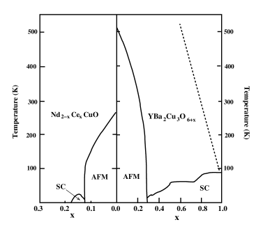
Figure 1: Phase diagram of the NCCO and the YBCO superconductors.

To date, a number of different HTSC materials have been discovered. The most studied of these include the hole doped $La_{2-x}Sr_{x}CuO_{4+\delta}$ (LSCO), $YBa_{2}Cu_{3}O_{6+\delta}$ (YBCO), $Bi_{2}Sr_{2}CaCu_{2}O_{8+\delta}$ (BSCO), and $Tl_{2}Ba_{2}CuO_{6+\delta}$ (TBCO) materials and the electron doped $Nd_{2-x}Ce_{x}CuO_{4}$ (NCCO) material. All these materials have two dimensional (2D) $CuO_{2}$ planes and display an antiferromagnetic (AF) insulating phase at half-filling. The magnetic properties of this insulating phase are well approximated by the AF Heisenberg model with spin $S=1/2$ and an AF exchange constant $J\sim 100meV$. The Neel temperature for the three dimensional AF ordering is approximately given by $T_{N}\sim 300-500K$. The HTSC material can be doped either by holes or by electrons. In the doping range of $5\%\lesssim x\lesssim 15\%$, there is an SC phase, which has a dome-like shape in the temperature versus doping plane. The maximal SC transition temperature, $T_{c}$, is of the order $100K$. The three doping regimes are divided by the maximum of the dome and are called the underdoped, optimally doped, and overdoped regimes, respectively. The generic phase diagram of HTSC is shown in Fig. 1.

One of the main questions concerning the HTSC phase diagram is the transition region between the AF and SC phases. Partly because of the complicated material chemistry in this regime, there is no universal agreement among different experiments. Different experiments indicate several different possibilities, including phase separation with an inhomogeneous density distribution Howald et al. (2001); Lang et al. (2002), uniform mixed phase between AF and SCBrewer et al. (1988); Miller et al. (2003), and periodically ordered spin and charge distributions in the form of stripes or checkerboardsTranquada et al. (1995).

The phase diagram of the HTSC cuprates also contains a regime with anomalous behavior conventionally called the pseudogap phase. This region of the phase diagram is indicated by the dashed line in Fig. 1. In conventional superconductors, a pairing gap opens up at $T_{c}$. In a large class of HTSC cuprates, however, a gap, which can be observed in a variety of spectroscopic experiments, starts to open up at a temperature $T^{*}$, much higher than $T_{c}$. Many experiments indicate that the pseudogap “phase” is not a true thermodynamical phase but rather a precursor toward a crossover behavior. The phenomenology of the pseudogap behavior is extensively reviewed inTimusk and Statt (1999); Tallon and Loram (2001).

The SC phase of the HTSC has a number of striking properties not shared by conventional superconductors. First of all, phase sensitive experiments indicate that the SC phase of most cuprates has $d$-wave like pairing symmetryHarlingen (1995); Tsuei and Kirtley (2000). This is also supported by the photoemission experiments, which show the existence of the nodal points in the quasiparticle gap Campuzano et al. (2002); Damascelli et al. (2003). Neutron scattering experiments find a new type of collective mode, carrying spin one, lattice momentum close to $(\pi,\pi)$ and a resolution limited sharp resonance energy around $20\sim 40meV$. Most remarkably, this resonance mode appears only below $T_{c}$ in the optimally doped cuprates. It has been found in a number of materials, including the YBCO, BSCO and the TBCO classes of materialsRossat-Mignod et al. (1991b); Mook et al. (1993); Fong et al. (1995); Dai et al. (1996); Fong et al. (1996); Mook et al. (1998); Dai et al. (1998); Fong et al. (2000, 1999); He et al. (2001, 2002). Another property uniquely different from the conventional superconductors is the vortex state. Most HTSC are type II superconductors in which the magnetic field can penetrate into the SC state in the form of a vortex lattice, with the SC order being destroyed at the center of the vortex core. In conventional superconductors, the vortex core is filled by normal metallic electrons. However, a number of different experimental probes, including neutron scattering, muon spin resonance ($\mu$sR), and nuclear magnetic resonance (NMR) have shown that the vortex cores in the HTSC cuprates are antiferromagnetic, rather than normal metallicLevi (2002); Katano et al. (2000); Lake et al. (2001, 2002); Miller et al. (2002); Mitrovic et al. (2001); Khaykovich et al. (2002); Mitrovic et al. (2003); Kakuyanagi et al. (2003); Kang et al. (2003); Fujita et al. (2003). This phenomenon has been observed in almost all HTSC materials, including LSCO, YBCO, TBCO and NSCO; thus, it appears to be a universal property of the HTSC cuprates.

The HTSC materials also have highly unusual transport properties. While conventional metals have a $T^{2}$ dependence of resistivity, in accordance with the predictions of the Fermi liquid theory, the HTSC materials display a linear $T$ dependence of the resistivity near optimal doping. This linear $T$ dependence extends over a wide temperature window and seems to be universal among most of the cuprates. When the underdoped or sometimes optimally doped SC state is destroyed by applying a high magnetic field, the resulting “normal state” is not a conventional conducting stateAndo et al. (1995, 1996); Boebinger et al. (1996); Hill et al. (2001) but exhibits insulating like behavior, at least along the $c$ axis, i.e. the axis perpendicular to the $CuO_{2}$ planes. This phenomenon may be related to the insulating AF vortices mentioned in the previous paragraph.

The HTSC materials attracted great attention because of the high SC transition temperature. However, many of the striking properties discussed above are also shared by other materials, which have a similar phase diagram but typically with much reduced temperature and energy scales. The 2D organic superconductor $\kappa-(BEDT-TTF)_{2}X$ (X=anion) display a similar phase diagram in the temperature versus pressure plane, where a direct first order transition between the AF and SC phases can be tuned by pressure or magnetic fieldLefebvre et al. (2000); Taniguchi et al. (2003); Singleton and Mielke (2002). In this system, the AF transition temperature is approximately $T_{N}\sim 30K$, while the SC transition temperature is $T_{c}\sim 14K$. In heavy fermion compounds $CeCu_{2}(Si_{1-x}Ge_{x})_{2}$Kitaoka et al. (2001), $CePd_{2}Si_{2}$ and $CeIn_{3}$Mathur et al. (1998), the SC phase also appears near the boundary to the AF phase. In all these systems, even though the underlying solid state chemistries are rather different, the resulting phase diagrams are strikingly similar and robust. This similarity suggests that the overall feature of all these phase diagrams is controlled by a single energy scale. Different classes of materials differ only by this overall energy scale. Another interesting example of competing AF and SC can be found in quasi-one-dimensional Bechgaard salts. The most well studied material from this family, $(TMTSF)_{2}PF_{6}$, is an AF insulator at ambient pressure and becomes a triplet SC above a certain critical pressure Jerome et al. (1980); Vuletic et al. (2002); Lee et al. (1997, 2003).

The discovery of HTSC has greatly stimulated the theoretical understanding of superconductivity in strongly correlated systems. Since the theoretical literature is extensive, the readers are referred to a number of excellent reviews and representative articlesAnderson (1997); Inui et al. (1988); Scalapino (1995); Schrieffer et al. (1989); Abrikosov (2000); Chubukov et al. (2002); Laughlin (2002); Sachdev (2002a); Zaanen (1999b); Chakravarty et al. (2001); Carlson et al. (2002); Franz et al. (2002b); Ioffe and Millis (2002); Varma (1999); Senthil and Fisher (2001); Wen and Lee (1996); Dagotto (1994); Norman and Pepin (2003); Balents et al. (1998); Shen et al. (2002); Anderson et al. (2003); Fu et al. (2004). The present review article focuses on a particular theory, which unifies the AF and SC phases of the HTSC cuprates based on an approximate $SO(5)$ symmetryZhang (1997). The $SO(5)$ theory draws its inspiration from the successful application of symmetry principles in theoretical physics. All fundamental laws of Nature are statements about symmetry. Conservation of energy, momentum and charge are direct consequences of global symmetries. The form of fundamental interactions are dictated by local gauge symmetries. Symmetry unifies apparently different physical phenomena into a common framework. For example, electricity and magnetism were discovered independently and viewed as completely different phenomena before the 19th century. Maxwell’s theory and the underlying relativistic symmetry between space and time unified the electric field, $\vec{E}$, and the magnetic field, $\vec{B}$, into a common electromagnetic field tensor, $F_{\mu\nu}$. This unification shows that electricity and magnetism share a common microscopic origin and can be transformed into each other by going to different inertial frames. As discussed in the introduction, the two robust and universal ordered phases of the HTSC are the AF and SC phases. The central question of HTSC concerns the transition from one phase to the other as the doping level is varied.

The $SO(5)$ theory unifies the three dimensional AF order parameter $(N_{x},N_{y},N_{z})$ and the two dimensional SC order parameter $(Re\Delta,Im\Delta)$ into a single, five dimensional order parameter called the superspin, in a way similar to the unification of electricity and magnetism in Maxwell’s theory:

$$F_{\mu\nu}\!=\!\left(\begin{array}[]{cccc}0&&&\\ E_{x}&0&&\\ E_{y}&B_{z}&0&\\ E_{z}&-B_{y}&B_{x}&0\end{array}\right)\ \ \ \Leftrightarrow\ \ \ n_{a}\!=\!\left(\begin{array}[]{c}Re\Delta\\ N_{x}\\ N_{y}\\ N_{z}\\ Im\Delta\\ \end{array}\right).$$ (10)

This unification relies on the postulate that a common microscopic interaction is responsible for both AF and SC in the HTSC cuprates and related materials. A well-defined $SO(5)$ transformation rotates one form of the order into another. Within this framework, the mysterious transition from the AF to SC phase as a function of doping is explained in terms of a rotation in the five dimensional order parameters space. Symmetry principles are not only fundamental and beautiful, but they are also practically useful in extracting information from a strongly interacting system, which can be tested quantitatively. As seen in the examples applying the isospin $SU(2)$ and the $SU(3)$ symmetries to the strong interaction, some quantitative predictions can be made and tested even when the symmetry is broken. The approximate $SO(5)$ symmetry between the AF and SC phases has many direct consequences, which can be tested both numerically and experimentally. We shall discuss a number of these tests in this review article.

Historically, the $SO(5)$ theory concentrated on the competition between AF and SC orders in the high Tc cuprates. The idea of some order competing with superconductivity is common in several theories. The staggered flux or the $d$-density wave phase has been suggested in Refs. Affleck and Marston (1988); Wen and Lee (1996); Chakravarty et al. (2001), the spin-Peierls order has been discussed in Refs. Vojta and Sachdev (1999); Park and Sachdev (2001), and spin and charge density wave orders have been considered in Refs. Zaanen (1999a); Kivelson et al. (2001); Zhang et al. (2002). The $SO(5)$ theory extends simple consideration of the competition between AF and SC in the cuprates by unifying the two order parameters using a larger symmetry and examining consequences of such symmetry.

The microscopic interactions in the HTSC materials are highly complex, and the resulting phenomenology is extremely rich. The $SO(5)$ theory is motivated by a confluence of the phenomenological top-down approach with the microscopic bottom-up approach, as discussed below.

The top-down approach: Upon first glance at the phase diagram of the HTSC cuprates, one is immediately impressed by its striking simplicity; there are only three universal phases in the phase diagram of all HTSC cuprates: the AF, the SC and the metallic phases, all with homogeneous charge distributions. However, closer inspection reveals a bewildering complexity of other possible phases, which may not be universally present in all HTSC cuprates, and which may have inhomogeneous charge distributions. Because of this complexity, formulating a universal theory of HTSC is a formidable challenge. The strategy of the $SO(5)$ theory can be best explained with an analogy: we see a colorful world around us, but the entire rainbow of colors is composed of only three primary colors. In the $SO(5)$ theory, the superspin plays the role of the primary colors. A central macroscopic hypothesis of the $SO(5)$ theory is that the ground state and the dynamics of collective excitations in various phases of the HTSC cuprates can be described in terms of the spatial and temporal variations of the superspin. This is a highly constraining and experimentally testable hypothesis, since it excludes many possible phases. It does include a homogeneous state in which AF and SC coexist microscopically. It includes states with spin and charge density wave orders, such as stripe phases, checkerboards and AF vortex cores, which can be obtained from spatial modulations of the superspin. It also includes quantum disordered ground states and Cooper pair density wave, which can be obtained from the temporal modulation of the superspin. The metallic Fermi liquid state on the overdoped side of the HTSC phase diagram seems to share the same symmetry as the high temperature phase of the underdoped cuprates. Therefore, they can also be identified with the disordered state of the superspin, although extra care must be given to treat the gapless fermionic excitations in that case. If this hypothesis is experimentally proven to be correct, a great simplicity emerges from the complexity: a full dynamical theory of the superspin field can be the universal theory of the HTSC cuprates. Part of this review article is devoted to describing and classifying phases which can be obtained from this theory. This top-down approach focuses on the low energy collective degrees of freedom and takes as the starting point a theory expressed exclusively in terms of these collective degrees of freedom. This is to be contrasted with the conventional approach based on weak coupling Fermi liquid theory, of which the BCS theory is a highly successful example. For an extensive discussion on the relative merits of both approaches for the HTSC problem, we refer the readers to an excellent, recent review article in Ref. Carlson et al. (2002).

The $SO(5)$ theory is philosophically inspired by the Landau-Ginzburg (LG) theory. The LG theory is a highly successful phenomenological theory, in which one first makes observations of the phase diagram, introduces one order parameter for each broken symmetry phase and constructs a free energy functional by expanding in terms of different order parameters (a review of earlier work based on this approach is given in Ref. Vonsovsky et al. (1982)). However, given the complexity of interactions and phases in the cuprates, introducing one order parameter for each phase with unconstrained parameters would greatly compromise the predictive power of theory. The $SO(5)$ theory extends the LG theory in several important directions. First, it postulates an approximately symmetric interaction potential between the AF and the SC phases in the underdoped regime of the cuprates, thereby greatly constraining theoretical model building. Second, it includes a full set of dynamic variables canonically conjugate to the superspin order parameters, including the total spin, the total charge and the so called $\pi$ operators. Therefore, unlike the classical LG theory, which only contains the classical order parameter fields without their dynamically conjugate variables, the $SO(5)$ theory is capable of describing quantum disordered phases and the quantum phase transitions between these phases. Because the quantum disordered phases are described by the degrees of freedom canonically conjugate to the classical order parameters, a definite relationship, the so-called $SO(5)$ orthogonality relation, exists between them, which can give highly constrained theoretical predictions. Therefore, in this sense, the $SO(5)$ theory makes great use of the LG theory but also goes far beyond in making more constrained and more powerful predictions which are subject to experimental falsifications.

The bottom-up approach: Soon after the discovery of the HTSC cuprates, AndersonAnderson (1987) introduced the repulsive Hubbard model to describe the electronic degrees of freedom in the $CuO_{2}$ plane. Its low energy limit, the $t-J$ model, is defined byZhang and Rice (1988)

$$H=-t\sum_{\langle x,x^{\prime}\rangle}c^{\dagger}_{\sigma}(x)c_{\sigma}(x^{\prime})+J\sum_{\langle x,x^{\prime}\rangle}\vec{S}(x)\cdot\vec{S}(x^{\prime}),$$ (11)

where the $t$ term describes the hopping of an electron with spin $\sigma$ from a site $x^{\prime}$ to its nearest neighbor $x$, with double occupancy removed, and the $J$ term describes the nearest neighbor spin exchange interaction. The main merit of these models does not lie in the microscopic accuracy and realism but rather in the conceptual simplicity. However, despite their simplicity, these models are still very hard to solve, and their phase diagram cannot be compared directly with experiments.

The $t-J$ model certainly contains AF at half-filling. While it is still not fully settled whether it has $d$-wave SC ground state with a high transition temperature Pryadko et al. (2003), it is reasonably convincing that it has strong $d$-wave pairing fluctuationsSorella et al. (2002). Therefore, it is plausible that a small modification could give a robust SC ground state. The basic microscopic hypothesis of the $SO(5)$ theory is that AF and SC states arise from the same interaction with a common energy scale of $J$. This common energy scale justifies the treatment of AF and SC on equal footing and is also the origin of an approximate $SO(5)$ symmetry between these two phases. By postulating an approximate symmetry between the AF and SC phases, and by systematically testing this hypothesis experimentally and numerically, the question of the microscopic mechanism of HTSC can also be resolved. In this context, early numerical diagonalizations showed that the low-lying states of the $t-J$ model fit into irreducible representations of the $SO(5)$ symmetry group Eder et al. (1998). If the $SO(5)$ symmetry is valid, then HTSC shares a common microscopic origin with the AF, which is a well understood phenomenon.

The basic idea is to solve these models by two steps. The first step is a renormalization group transformation, which maps these microscopic models to an effective superspin model on a plaquette, typically of the size of $2a\times 2a$ or larger. This step determines the form and the parameters of the effective models. The next step is to solve the effective model either through accurate numerical calculations or tractable analytical calculations.

There is a systematic method to carry out the first step. Using the contractor-renormalization-group (CORE)Morningstar and Weinstein (1996) approach, Altman and AuerbachAltman and Auerbach (2002) derived the projected $SO(5)$ model from the Hubbard and the $t-J$ model. Within the approximations studied to date, a simple and consistent picture emerges. There are only five low energy states on a coarse grained lattice site, namely a spin singlet state and a spin triplet state at half-filling and a $d$-wave hole pair state with two holes. These states correspond exactly to the local and dynamical superspin degrees of freedom hypothesized in the top-down approach. The resulting effective $SO(5)$ superspin model, valid near the underdoped regime, only contains bosonic degrees of freedom. This model can be studied by quantum Monte-Carlo simulations up to very large sizes, and the accurate determination of the phase diagram is possible (in contrast to the Hubbard and $t-J$ models) because of the absence of the minus sign problems. Once the global phase diagrams are determined, fermionic excitations in each phase can also be studied by approximate analytic methods. Within this approach, the effective $SO(5)$ superspin model derived from the microscopic physics can give a realistic description of the phenomenology and phase diagram of the HTSC cuprates and account for many of their physical properties Dorneich et al. (2002b, a). This agreement can be further tested, refined and possibly falsified. This approach can be best summarized by the following block diagram:

Hubbard and t-J	coarse graining	Quantum SO(5)		analytical and numerical		Phase diagram
model	$\Longrightarrow$	model		$\Longrightarrow$		Collective modes
of the electron	transformation	of the superspin		calculations		other experiments…

While the practical execution of the first step already introduces errors and uncertainties, we need to remember that the Hubbard and the $t-J$ models are effective models themselves, and they contain errors and uncertainties compared with the real materials. The error involved in our coarse grain process is not inherently larger than the uncertainties involved in deriving the Hubbard and the $t-J$ models from more realistic models. Therefore, as long as we study a reasonable range of the parameters in the second step and compare them directly with experiments, we could determine these parameters.

This review is intended as a self-contained introduction to a particular theory of the HTSC cuprates and related materials and is organized as follows. Section II describes three toy models which introduce some important concepts used in the rest of the article. Section III introduces the concept of the $SO(5)$ superspin and its symmetry transformation, as well as effective dynamical models of the superspin. The global phase diagram of the $SO(5)$ model is discussed and solved numerically in section IV. Section V introduces exact $SO(5)$ symmetric microscopic models, the numerical tests of the $SO(5)$ symmetry in the $t-J$ and Hubbard models, and the Altman-Auerbach procedure of deriving the $SO(5)$ model from microscopic models of the HTSC cuprates. Section VI discusses the $\pi$ resonance model and the microscopic mechanism of HTSC. Finally, in section VII, we discuss experimental predictions of the $SO(5)$ theory and comparisons with the tests performed so far. The readers are assumed to have general knowledge of quantum many body physics and are referred to several excellent textbooks for pedagogical introductions to the basic concepts and theoretical toolsAnderson (1997); Abrikosov et al. (1993); Pines and Nozieres (1966); Schrieffer (1964); Tinkham (1995); Auerbach (1994); Sachdev (2000).

II THE SPIN-FLOP AND THE MOTT INSULATOR TO SUPERCONDUCTOR TRANSITION

Before presenting the full $SO(5)$ theory, let us first discuss a much simpler class of toy models, namely the anisotropic Heisenberg model in a magnetic field, the hard-core lattice boson model and the negative $U$ Hubbard model. The low energy limits of this class of models are all equivalent to each other and can be described by a universal quantum field theory, the $SO(3)$ quantum non-linear sigma model. Although these models are simple to solve, they exhibit some of the key properties of the HTSC cuprates, including strong correlation, competition of different orders, low superfluid density near the insulating phase, maximum of $T_{c}$, and the pseudogap behavior.

The spin $1/2$ anisotropic AF Heisenberg model on a square lattice is described by the following Hamiltonian:

$$H=\sum_{\langle x,x^{\prime}\rangle}S^{z}(x)V(x,x^{\prime})S^{z}(x^{\prime})+J\sum_{\langle x,x^{\prime}\rangle}(S^{x}(x)S^{x}(x)+S^{y}(x)S^{y}(x))-B\sum_{x}S^{z}(x).$$ (12)

Here, $S^{\alpha}=\frac{1}{2}\tau^{\alpha}$ is the Heisenberg spin operators and $\tau^{\alpha}$ is the Pauli matrix. $J$ describes the nearest-neighbor exchange of the $xy$ components of the spin, while $V(x,x^{\prime})$ describes the $z$ component of the spin interaction. We shall begin by considering only the nearest neighbor (denoted by $\langle x,x^{\prime}\rangle$) spin interaction $V$. $B$ is an external magnetic field. At the point of $B=0$ and $J=V$, this model enjoys an $SO(3)$ symmetry generated by the total spin operators:

$$S^{\alpha}=\sum_{x}S^{\alpha}(x)\ \ ,\ \ [S^{\alpha},S^{\beta}]=i\epsilon_{\alpha\beta\gamma}S^{\gamma}\ \ ,\ \ [H,S^{\alpha}]=0..$$ (13)

The order parameter in this problem is the Neel operator, which transforms according to the vector representation of the $SO(3)$ group

$$N^{\alpha}=\sum_{x}(-)^{x}S^{\alpha}(x)\ \ ,\ \ [S^{\alpha},N^{\beta}]=i\epsilon_{\alpha\beta\gamma}N^{\gamma}.$$ (14)

Here $(-)^{x}=1$ if $x$ is on an even site and $(-)^{x}=-1$ if $x$ is on an odd site. The symmetry generators and the order parameters are canonically conjugate degrees of freedom, and the second part of Eq. (14) is similar to the Heisenberg commutation relation $[x,p]=i\hbar$ between the canonically conjugate position and momentum. Just like $p$ can be expressed as $\frac{\hbar}{i}\partial/\partial x$, one can express

$$S^{\alpha}=i\epsilon^{\alpha\beta\gamma}N^{\beta}\frac{\partial}{\partial N^{\gamma}}\ \ ,\ \ N^{\alpha}S^{\alpha}=0,$$ (15)

where the second part of the equation, called the $SO(3)$ orthogonality relation, follows directly from the first. Both the symmetry algebra, the canonical conjugation and the orthogonality constraint are fundamental concepts important to the understanding of the dynamics and the phase diagram of the model.

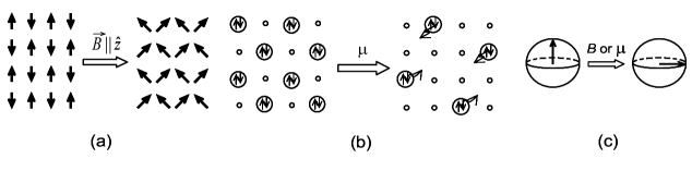
Figure 2: (a) The spin-flop transition of the XXZ Heisenberg model. (b) the Mott insulator to superfluid transition of the hard-core boson model or the $U<0$ Hubbard model. (c) Both can be described as the spin or the pseudospin flop transition in the $SO(3)$ non-linear $\sigma$ model, induced either by the magnetic field or the chemical potential.

Let us first consider the classical, mean field approximation to the ground state of the anisotropic Heisenberg model defined in Eq.(12). For $V>J$, the spins like to align antiferromagnetically along the $z$ direction. In the Ising phase, $S^{z}(x)=(-1)^{x}S$, the ground state energy per site is given by $e_{Ising}(B)=-\frac{zV}{2}S^{2}$, where $z$ is the coordination number, which is $4$ for the square lattice. Note that the energy is independent of the $B$ field in the Ising phase. For larger values of $B$, the spins “flop” into the $XY$ plane, and tilt uniformly toward the $Z$ axis. (See Fig. 2a). Such a spin-flop state is given by $S^{z}(x)=Scos\theta$ and $S^{x}(x)=(-1)^{x}Ssin\theta$. The minimal energy configuration is given by $cos\theta=B/zS(V+J)$, and the energy per site for this spin-flop state is $e_{XY}(B)=-zJS^{2}/2-B^{2}/2z(V+J)$. Comparing the energies of both states, we obtain the critical value of $B$ where the spin-flop transition occurs: $B_{c1}=zS\sqrt{V^{2}-J^{2}}$. On the other hand, we require $|cos\theta|\leq 1$, which implies a critical field $B_{c2}=zS(V+J)$ at which $|cos\theta|=1$, and the staggered order parameter vanishes. Combining these phase transition lines, we obtain the “class $B$” transition in the ground state phase diagram depicted in the $B$-$J/V$ plane (see Fig. 3a). Here and later in the article, the “class $B$” transition refers to the transition induced by the chemical potential or the magnetic field. At the $SO(3)$ symmetric point, $V=J$ and $B_{c1}=0$. For $V<J$, the ground state has XY order even at $B=0$, and there is no spin-flop transition as a function of the magnetic field $B$. The Ising to XY transition can also be tuned by varying $J/V$ at $B=0$, and the phase transition occurs at the special $SO(3)$ symmetric Heisenberg point. This type of transition is also depicted in Fig. 3a and will be called “class $A$” transition in this paper.

The spin $1/2$ Heisenberg model can be mapped to a hard-core boson model, defined by the following Hamiltonian:

$$H=\sum_{\langle x,x^{\prime}\rangle}n(x)V(x,x^{\prime})n(x^{\prime})-\frac{1}{2}J\sum_{\langle x,x^{\prime}\rangle}(b^{\dagger}(x)b(x^{\prime})+h.c.)-\mu\sum_{x}n(x).$$ (16)

Here $b(x)$ and $b^{\dagger}(x)$ are the hard-core boson annihilation and creation operators and $n(x)=b^{\dagger}(x)b(x)$ is the boson density operator. In this context, $V$, $J$ and $\mu$ describe the interaction, hopping and the chemical potential energies, respectively. There are two states per site; $|1\rangle$ and $|0\rangle$ denote the filled and empty boson states, respectively. They can be identified with the spin up $|\uparrow\rangle$ and the spin down $|\downarrow\rangle$ states of the Heisenberg model. The operators in the two theories can be identified as follows:

$$b(x)^{\dagger}=(-)^{x}(S^{x}(x)+iS^{y}(x))\ \ \ b(x)=(-)^{x}(S^{x}(x)-iS^{y}(x))\ \ \ n(x)=S^{z}(x)+\frac{1}{2}.$$ (17)

We see that these two models are identical to each other when $\mu=B+zV/2$. From this mapping, we see that the spin-flop phase diagram has another interpretation: the Ising phase is equivalent to the Mott insulating phase of bosons with a charge-density-wave (CDW) order in the ground state. The XY phase is equivalent to the superfluid phase of the bosons. The two paramagnetic states correspond to the full and empty states of the bosons. While Heisenberg spins are intuitively associated with the $SO(3)$ spin rotational symmetry, lattice boson models generically have only a $U(1)$ symmetry generated by the total number operator $N=\sum_{x}n(x)$, which transforms the boson operators by a phase factor: $b^{\dagger}(x)\rightarrow e^{i\alpha}b^{\dagger}(x)$ and $b(x)\rightarrow e^{-i\alpha}b(x)$. From this point of view, it is rather interesting and non-trivial that the boson model can also have an additional $SO(3)$ symmetry at the special point $J=V$ because of its equivalence to the Heisenberg model.

Having discussed the Heisenberg spin model and the lattice boson models, let us now consider a fermion model, namely the negative $U$ Hubbard model, defined by the Hamiltonian

$$H=-t\sum_{\langle x,x^{\prime}\rangle}(c^{\dagger}_{\sigma}(x)c_{\sigma}(x^{\prime})+h.c.)+U\sum_{x}(n_{\uparrow}(x)-\frac{1}{2})(n_{\downarrow}(x)-\frac{1}{2})-\mu\sum_{x}n_{\sigma}(x),$$ (18)

where $c_{\sigma}(x)$ is the fermion operator and $n_{\sigma}(x)=c^{\dagger}_{\sigma}(x)c_{\sigma}(x)$ is the electron density operator at site $x$ with spin $\sigma$. $t$, $U$ and $\mu$ are the hopping, interaction and the chemical potential parameters respectively. The Hubbard model has a pseudospin $SU(2)$ symmetry generated by the operators

$$\eta^{-}=\sum_{x}(-)^{x}c_{\uparrow}(x)c_{\downarrow}(x)\ \ ,\ \ \eta^{+}=(\eta^{-})^{\dagger}\ \ ,\ \ \eta^{z}=\frac{1}{2}\sum_{\sigma}(n_{\sigma}(x)-\frac{1}{2})\ \ ,\ \ [\eta^{\alpha},\eta^{\beta}]=i\epsilon_{\alpha\beta\gamma}\eta^{\gamma}.$$ (19)

where $\eta^{\pm}=\eta^{x}\pm i\eta^{y}$ and $\alpha=x,y,z$, as before. Yang and ZhangYang (1989); Yang and Zhang (1990); Zhang (1990) pointed out that these operators commute with the Hubbard Hamiltonian when $\mu=0$ ( i.e. $[H,\eta^{\alpha}]=0$); therefore, they form the symmetry generators of the model. Combined with the standard $SU(2)$ spin rotational symmetry, the Hubbard model enjoys a $SO(4)=SU(2)\otimes SU(2)/Z_{2}$ symmetry. This symmetry has important consequences in the phase diagram and the collective modes in the system. In particular, it implies that the SC and CDW orders are degenerate at half-filling. The SC and the CDW order parameters are defined by

$$\Delta^{-}=\sum_{i}c_{i\uparrow}c_{i\downarrow}\ \ ,\ \ \Delta^{+}=(\Delta^{-})^{\dagger}\ \ ,\ \ \Delta^{z}=\frac{1}{2}\sum_{i\sigma}(-1)^{i}n_{i\sigma}\ \ ,\ \ [\eta^{\alpha},\Delta^{\beta}]=i\epsilon_{\alpha\beta\gamma}\Delta^{\gamma},$$ (20)

where $\Delta^{\pm}=\Delta^{x}\pm i\Delta^{y}$. The last equation above shows that the $\eta$ operators perform the rotation between the SC and CDW order parameters. Thus, $\eta^{\alpha}$ is the pseudospin generator and $\Delta^{\alpha}$ is the pseudospin order parameter. Just like the total spin and the Neel order parameter in the AF Heisenberg model, they are canonically conjugate variables. Since $[H,\eta^{\alpha}]=0$ at $\mu=0$, this exact pseudospin symmetry implies the degeneracy of SC and CDW orders at half-filling.

The phase diagram of the $U<0$ Hubbard model corresponds to a 1D slice of the 2D phase diagram, as depicted in Fig.3a. The exact pseudospin symmetry implies that the “class $B$” transition line for the $U<0$ Hubbard model exactly touches the tip of the Mott lobe, as shown by the $B^{\prime}$ line in Fig.3a. At $\mu=0$, SC and CDW are exactly degenerate, and they can be freely rotated into each other. For $\mu\neq 0$, the system is immediately rotated into the SC state. One can add additional interactions in the Hubbard model, such as a nearest neighbor repulsion, which breaks the $SU(2)$ pseudospin rotation symmetry even at $\mu=0$. In this case, the pseudospin anisotropy either picks the CDW Mott insulating phase or the SC phase at half-filling. By adjusting the nearest neighbor interaction, one can move the height of the “class $B$” transition line.

We have seen that the hard-core boson model is equivalent to the Heisenberg model because of the mapping (17). The $U<0$ model, on the other hand, is only equivalent to the Heisenberg model in the low energy limit. In fact, it is equivalent to a $U>0$ Hubbard at half-filling in the presence of a Zeeman magnetic field. The ground state of the half-filled Hubbard model is always AF; therefore, its low energy limit is the same as that of the Heisenberg model in a magnetic field. All three models are constructed from very different microscopic origins. However, they all share the same phase diagram, symmetry group and low energy dynamics. In fact, these universal features can all be captured by a single effective quantum field theory model, namely the $SO(3)$ quantum non-linear $\sigma$ model. This model can be derived as an effective model from the microscopic models introduced earlier or it can be constructed purely from symmetry principles and the associated operator algebra as defined in Eq. (13) and (14). The fact that both derivations yield the same model is hardly surprising, since the universal features of all these models are direct consequences of the symmetry.

The $SO(3)$ non-linear $\sigma$ model is defined by the following Lagrangian density for a unit vector field $n_{\alpha}$ with $n^{2}_{\alpha}=1$:

$${\cal L}=\frac{\chi}{2}\omega^{2}_{\alpha\beta}-\frac{\rho}{2}(\partial_{i}n_{\alpha})^{2}-V(n)\ \ ,\ \ \omega_{\alpha\beta}=n_{\alpha}(\partial_{t}n_{\beta}-iB_{\beta\gamma}n_{\gamma})-(\alpha\leftrightarrow\beta),$$ (21)

where the Zeeman magnetic field is given by $B_{\alpha}=\frac{1}{2}\epsilon_{\alpha\beta\gamma}B_{\beta\gamma}$. Without loss of generality, we pick the magnetic field $B$ to be along the $z$ direction. $\chi$ and $\rho$ are the susceptibility and stiffness parameters and $V(n)$ is the anisotropy potential, which can be taken as $V(n)=-\frac{g}{2}n_{z}^{2}$. Exact $SO(3)$ symmetry is obtained when $g=B=0$. $g>0$ corresponds to easy axis anisotropy or $J/V<1$ in the Heisenberg model. $g<0$ corresponds to easy plane anisotropy or $J/V>1$ in the phase diagram of Fig.3. In the case of $g>0$, there is a phase transition as a function of $B$. To see this, let us expand the first term in (21) in the presence of the $B$ field. The time independent part contributes to an effective potential $V_{eff}=V(n)-\frac{B^{2}}{2}(n_{x}^{2}+n_{y}^{2})$, from which we see that there is a phase transition at $B_{c1}=\sqrt{g/\chi}$. For $B<B_{c1}$, the system is in the Ising phase, while for $B>B_{c1}$ the system is in the XY phase. Therefore, tuning $B$ for a fixed $g>0$ traces out the “class $B$” transition line, as depicted in Fig.3a. On the other hand, fixing $B=0$ and varying $g$ traces out the “class $A$” transition line, as depicted in Fig.3a. Therefore, we see that the $SO(3)$ non-linear $\sigma$ model has a similar phase diagram as the microscopic models discussed earlier. For a more detailed discussion of phase transitions in $SO(3)$ non-linear $\sigma$ models we refer the readers to an excellent review paper by Auerbach et alAuerbach et al. (2000).

In $D=2$, both the XY and the Ising phase can have a finite temperature phase transition into the disordered state. However, because of the Mermin-Wagner theorem, a finite temperature phase transition is forbidden at the point $B=g=0$, where the system has an enhanced $SO(3)$ symmetry. The finite temperature phase diagram is shown in Fig. 3b. Approaching from the SC side, the Kosterlitz-Thouless transition temperature $T_{XY}$ is driven to zero at the Mott to superfluid transition point $J/V=1$. In the 2D XY model, the superfluid density and the transition temperature $T_{XY}$ are related to each other by a universal relationshipNelson and Kosterlitz (1977); therefore, the vanishing of $T_{XY}$ also implies the vanishing of the superfluid density as one approaches the Mott to superfluid transition. Scalettar et alScalettar et al. (1989), Moreo and ScalapinoMoreo and Scalapino (1991) have performed extensive quantum Monte Carlo simulation in the negative $U$ Hubbard model and have indeed concluded that the superfluid density vanishes at the symmetric point. The $SO(3)$ symmetric point leads to a large regime below the mean field transition temperature where fluctuations dominate. The single particle spectral function of the 2D attractive Hubbard model has been studied extensively by Allen et alAllen et al. (1999) near half-filling. They identified the pseudogap behavior in the single particle density of states within this fluctuation regime. Based on this study, they argued that the pseudogap behavior is not only a consequence of the SC phase fluctuationsDoniach and Inui (1990); Emery and Kivelson (1995); Uemura (2002) but also a consequence of the full $SO(3)$ symmetric fluctuations, which also include the fluctuations between the SC and the CDW phases. Fig. 3c shows the generic finite temperature phase diagram of these $SO(3)$ models. In this case, the Ising and the XY transition temperatures meet at a single bi-critical point $T_{bc}$, which has the enhanced $SO(3)$ symmetry. At the “class $A$” transition point $g=B=0$, the quantum dynamics is fully $SO(3)$ symmetric. On the other hand, at the “class $B$” transition point $T=T_{bc}$, only the static potential is $SO(3)$ symmetric. We shall return to a detailed discussion of this distinction in section III.3.

The pseudospin $SU(2)$ symmetry of the negative $U$ Hubbard model has another important consequence. Away from half-filling, the $\eta$ operators no longer commute with the Hamiltonian, but they are eigen-operators of the Hamiltonian, in the sense that

$$[H,\eta^{\pm}]=\mp 2\mu\eta^{\pm}.$$ (22)

Thus, the $\eta$ operators create well defined collective modes in the system. Since they carry charge $\pm 2$, they usually do not couple to any physical probes. However, in a SC state, the SC order parameter mixes the $\eta$ operators with the CDW operator $\Delta^{z}$, via Eq. (20). From this reasoning, ZhangZhang (1990, 1991); Demler et al. (1996) predicted a pseudo-Goldstone mode in the density response function at wave vector $(\pi,\pi)$ and energy $-2\mu$, which appears only below the SC transition temperature $T_{c}$. This prediction anticipated the neutron resonance mode later discovered in the HTSC cuprates; a detailed discussion shall be given in section VI.

From the toy models discussed in this section, we learned a few very important concepts. Competition between different orders can sometimes lead to enhanced symmetries at the multi-critical point. Universal properties of very different microscopic models can be described by a single quantum field theory constructed from the canonically conjugate symmetry generators and order parameters. The enhanced symmetry naturally leads to a small superfluid density near the Mott transition. The pseudogap behavior in the single particle spectrum can be attributed to the enhanced symmetry near half-filling and new types of collective Goldstone modes can be predicted from the symmetry argument. All these behaviors are reminiscent of the experimental observations in the HTSC cuprates. The simplicity of these models on the one hand and the richness of the phenomenology on the other inspired the $SO(5)$ theory, which we shall discuss in the following sections.

III THE SO(5) GROUP AND EFFECTIVE THEORIES

III.1 Order parameters and SO(5) group properties

The $SO(3)$ models discussed in the previous section give a nice description of the quantum phase transition from the Mott insulating phase with CDW order to the SC phase. However, these simple models do not have enough complexity to describe the AF insulator at half-filling and the $d$-wave SC order away from half-filling. Therefore, a natural step is to generalize these models so that the Mott insulating phase with the scalar CDW order parameter is replaced by a Mott insulating phase with the vector AF order parameter. The pseudospin $SO(3)$ symmetry group considered previously arises from the combination of one real scalar component of the CDW order parameter with one complex or two real components of the SC order parameter. After replacing the scalar CDW order parameter by the three components of the AF order parameter and combining them with the two components of the SC order parameters, we are naturally led to consider a five component order parameter vector and the $SO(5)$ symmetry group which transforms it.

In section II, we introduced the crucial concept of order parameter and symmetry generator. Both of these concepts can be defined locally. In the case of the Heisenberg AF, at least two sites, for instance, $\vec{S}_{1}$ and $\vec{S}_{2}$, are needed to define the total spin $\vec{S}=\vec{S}_{1}+\vec{S}_{2}$ and the Neel vector $\vec{N}=\vec{S}_{1}-\vec{S}_{2}$. Similarly, it is simplest to define the concept of the $SO(5)$ symmetry generator and order parameter on two sites with fermion operators $c_{\sigma}$ and $d_{\sigma}$, respectively, where $\sigma=1,2$ is the usual spinor index. The AF order parameter operator can be defined naturally in terms of the difference between the spins of the $c$ and $d$ fermions as follows:

$$N^{\alpha}=\frac{1}{2}(c^{\dagger}\tau^{\alpha}c-d^{\dagger}\tau^{\alpha}d)\ \ ,\ \ n_{2}\equiv N_{1}\ \ ,\ \ n_{3}\equiv N_{2}\ \ ,\ \ n_{4}\equiv N_{3}.$$ (23)

In view of the strong on-site repulsion in the cuprate problem, the SC order parameter should be defined on a bond connecting the $c$ and $d$ fermions. We introduce

$$\Delta^{\dagger}=\frac{-i}{2}c^{\dagger}\tau^{y}d^{\dagger}=\frac{1}{2}(-c_{\uparrow}^{\dagger}d_{\downarrow}^{\dagger}+c_{\downarrow}^{\dagger}d_{\uparrow}^{\dagger})\ \ ,\ \ n_{1}\equiv\frac{\left(\Delta^{\dagger}+\Delta\right)}{2}\ \ ,\ \ n_{5}\equiv\frac{\left(\Delta^{\dagger}-\Delta\right)}{2i}.$$ (24)

We can group these five components together to form a single vector $n_{a}=(n_{1},n_{2},n_{3},n_{4},n_{5})$, called the superspin since it contains both superconducting and antiferromagnetic spin components. The individual components of the superspin are explicitly defined in the last parts of Eqs. (23) and (24).

The concept of the superspin is useful only if there is a natural symmetry group acting on it. In this case, since the order parameter is five dimensional, it is natural to consider the most general rotation in the five dimensional order parameter space spanned by $n_{a}$. In three dimensions, three Euler angles are needed to specify a general rotation. In higher dimensions, a rotation is specified by selecting a plane and an angle of rotation within this plane. Since there are $n(n-1)/2$ independent planes in $n$ dimensions, the group $SO(n)$ is generated by $n(n-1)/2$ elements, specified in general by antisymmetric matrices $L_{ab}=-L_{ba}$, with $a=1,..,n$. In particular, the $SO(5)$ group has ten generators. The total spin and the total charge operators,

$$S_{\alpha}=\frac{1}{2}(c^{\dagger}\tau^{\alpha}c+d^{\dagger}\tau^{\alpha}d)\ \ ,\ \ Q=\frac{1}{2}(c^{\dagger}c+d^{\dagger}d-2),$$ (25)

perform the rotation of the AF and SC order parameters within each subspace. In addition, there are six so-called $\pi$ operators, first introduced by Demler and ZhangDemler and Zhang (1995), defined by

$$\pi^{\dagger}_{\alpha}=-\frac{1}{2}c^{\dagger}\tau^{\alpha}\tau^{y}d^{\dagger}\ \ ,\ \ \pi_{\alpha}=(\pi^{\dagger}_{\alpha})^{\dagger}.$$ (26)

They perform the rotation from AF to SC and vice versa. These infinitesimal rotations are defined by the commutation relations

$$[\pi^{\dagger}_{\alpha},N_{\beta}]=i\delta_{\alpha\beta}\Delta^{\dagger}\ \ ,\ \ [\pi^{\dagger}_{\alpha},\Delta]=iN_{\alpha}.$$ (27)

The total spin components $S_{\alpha}$, the total charge $Q$, and the six $\pi$ operators form the ten generators of the $SO(5)$ group.

The superspin order parameters $n_{a}$, the associated $SO(5)$ generators $L_{ab}$, and their commutation relations can be expressed compactly and elegantly in terms of the $SO(5)$ spinor and the five Dirac $\Gamma$ matrices. The four component $SO(5)$ spinor is defined by

$$\Psi_{\mu}=\left(\begin{array}[]{c}c_{\sigma}\\ d^{\dagger}_{\sigma}\end{array}\right).$$ (30)

They satisfy the usual anti-commutation relations

$$\{\Psi^{\dagger}_{\mu},\Psi_{\nu}\}=\delta_{\mu\nu}\ \ ,\ \ \{\Psi_{\mu},\Psi_{\nu}\}=\{\Psi^{\dagger}_{\mu},\Psi^{\dagger}_{\nu}\}=0.$$ (31)

Using the $\Psi$ spinor and the five Dirac $\Gamma$ matrices (see appendix A), we can express $n_{a}$ and $L_{ab}$ as

$$n_{a}=\frac{1}{2}\Psi^{\dagger}_{\mu}\Gamma^{a}_{\mu\nu}\Psi_{\nu}\ \ ,\ \ L_{ab}=-\frac{1}{2}\Psi^{\dagger}_{\mu}\Gamma^{ab}_{\mu\nu}.\Psi_{\nu}$$ (32)

The $L_{ab}$ operators forms the $SO(5)$ Lie algebra and satisfy the commutation relation

$$\left[L_{ab},L_{cd}\right]=-i(\delta_{ac}L_{bd}+\delta_{bd}L_{ac}-\delta_{ad}L_{bc}-\delta_{bc}L_{ad}).$$ (33)

The $n_{a}$ and the $\Psi_{\mu}$ operators form the vector and the spinor representations of the $SO(5)$ group, satisfying the equations

$$\left[L_{ab},n_{c}\right]=-i(\delta_{ac}n_{b}-\delta_{bc}n_{a})$$ (34)

and

$$\left[L_{ab},\Psi_{\mu}\right]=\frac{1}{2}\Gamma^{ab}_{\mu\nu}\Psi_{\nu}.$$ (35)

If we arrange the ten operators $S_{\alpha}$, $Q$ and $\pi_{\alpha}$ into $L_{ab}$’s by the following matrix form:

$$L_{ab} = \left(\begin{array}[]{ccccc}0&&&&\\ \pi^{\dagger}_{x}\!+\!\pi_{x}&0&&&\\ \pi^{\dagger}_{y}\!+\!\pi_{y}&-S_{z}&0&&\\ \pi^{\dagger}_{z}\!+\!\pi_{z}&S_{y}&-S_{x}&0&\\ Q&\frac{1}{i}(\pi^{\dagger}_{x}\!-\!\pi_{x})&\frac{1}{i}(\pi^{\dagger}_{y}\!-\!\pi_{y})&\frac{1}{i}(\pi^{\dagger}_{z}\!-\!\pi_{z})&0\end{array}\right)$$ (41)

and group $n_{a}$ as in Eqs. (23) and (24), we see that Eqs. (33) and (34) compactly reproduces all the commutation relations presented previously. These equations show that $L_{ab}$ and $n_{a}$ are the symmetry generators and the order parameter vectors of the $SO(5)$ theory. The commutation relation Eq. (34) is the $SO(5)$ generalization of the $SO(3)$ communication relation as given in Eqs. (14) and (20).

In systems where the unit cell naturally contains two sites, such as the ladder and the bi-layer systems, the complete set of operators $L_{ab}$, $n_{a}$ and $\Psi_{\mu}$ can be used to construct model Hamiltonians with the exact $SO(5)$ symmetry, as we will show in section V.1. In these models, local operators are coupled to each other so that only the total symmetry generators, obtained as the sum of local symmetry generators, commute with the Hamiltonian. For two dimensional models containing only a single layer, grouping the lattice into clusters of two sites would break lattice translational and rotational symmetry. In this case, it is better to use a cluster of four sites forming a square, which does not break rotational symmetry and can lead naturally to the definition of a $d$-wave pairing operatorZhang et al. (1999); Altman and Auerbach (2002). In this case, the $L_{ab}$, $n_{a}$ and $\Psi_{\mu}$ operators are interpreted as the effective low energy operators defined on a plaquette, which form the basis for an effective low energy $SO(5)$ theory, rather than the basis of a microscopic $SO(5)$ model.

Having introduced the concept of local symmetry generators and order parameters based in real space, we will now discuss definitions of these operators in momentum space. The AF and SC order parameters can be naturally expressed in terms of the microscopic fermion operators as

$$N^{\alpha}=\sum_{p}c_{p+\Pi}^{\dagger}\tau^{\alpha}c_{p}\ \ ,\ \ \Delta^{\dagger}=\frac{-i}{2}\sum_{p}d(p)c_{p}^{\dagger}\tau^{y}c_{-p}^{\dagger}\ \ ,\ \ d(p)\equiv cos(p_{x})-cos(p_{y}),$$ (42)

where $\Pi\equiv(\pi,\pi)$ and $d(p)$ is the form factor for the $d$ wave pairing operator in two dimensions. They can be combined into the five component superspin vector $n_{a}$ by using the same convention as before. The total spin and total charge operator are defined microscopically as

$$S_{\alpha}=\sum_{p}c_{p}^{\dagger}\tau^{\alpha}c_{p}\ \ ,\ \ Q=\frac{1}{2}\sum_{p}(c_{p}^{\dagger}c_{p}-1),$$ (43)

and the $\pi$ operators can be defined as

$$\pi^{\dagger}_{\alpha} = \sum_{p}g(p)c_{p+\Pi}^{\dagger}\tau^{\alpha}\tau^{y}c_{-p}^{\dagger}.$$ (44)

Here the form factor $g(p)$ needs to be chosen appropriately to satisfy the $SO(5)$ commutation relation (33). In the original formulation of the $SO(5)$ theory, ZhangZhang (1997) chose $g(p)=d(p)$. In this case, the $SO(5)$ symmetry algebra (33) only closes approximately near the Fermi surface. Later, HenleyHenley (1998) proposed the choice $g(p)=sgn(d(p))$(this construction requires introducing form factors for the AF order parameter as well). When the momentum space operators $S_{\alpha}$, $Q$ and $\pi^{\dagger}_{\alpha}$, as expressed in Eq. (43) and (44), are grouped into $L_{ab}$ according to Eq. (41), the symmetry algebra (33) closes exactly. However, the $\pi$-operators are no longer short ranged.

The $SO(5)$ symmetry generators perform the most general rotation among the five order parameters. The quantum numbers of the $\pi$ operators exactly patch up the difference in quantum numbers between the AF and SC order parameters, as shown in the Table I.

	charge	spin	momentum	internal angular momentum
$\Delta,\Delta^{\dagger}\ \textrm{or}\ n_{1},n_{5}$	$\pm 2$	0	0	d wave
$N^{\alpha}\ \textrm{or}\ n_{2,3,4}$	0	1	$(\pi,\pi)$	s wave
$\pi_{\alpha},\pi_{\alpha}^{\dagger}$	$\pm 2$	1	$(\pi,\pi)$	d wave

Table 1: Quantum numbers of the AF, the $d$-wave SC order parameters, and the $\pi$ operator. Since the $\pi$ operator rotates the AF and SC order parameters into each other, its quantum numbers patch up the difference between the AF and SC order parameters.

With the proper choice of the internal form factors, the $\pi$ operators rotate between the AF and SC order parameters according to (27). Analogous to the electro-magnetic unification presented in the introduction, the $\pi$ operators generate an infinitesimal rotation between the AF and SC order parameters similar to the infinitesimal rotation between the electric and the magnetic fields generated by the Lorentz transformation. These commutation relations play a central role in the $SO(5)$ theory and have profound implications on the relationship between the AF and SC order – they provide a basis to unify these two different types of order in a single framework. In the AF phase, the operator $N^{\alpha}$ acquires a nonzero expectation value, and the $\pi$ and SC operators become canonically conjugate variables in the sense of Hamiltonian dynamics. Conversely, in the SC phase the operator $\Delta$ acquires a nonzero expectation value, and the $\pi$ and AF operators become canonically conjugate variables. This canonical relationship is the key to understanding the collective modes in the $SO(5)$ theory and in HTSC.

The $SO(5)$ group is the minimal group to contain both AF and SC, the two dominant phases in the HTSC cuprates. However, it is possible to generalize this construction so that it includes other forms of order. For example, in Ref. Podolsky et al. (2004), it was demonstrated how one can combine AF and triplet SC using an $SO(4)$ symmetry Rozhkov and Millis (2002). Such a construction is useful for quasi-one-dimensional Bechgaard salts, which undergo a transition from an AF insulating state to a triplet SC state as a function of pressureJerome et al. (1980); Vuletic et al. (2002); Lee et al. (1997, 2003).

To define an $SO(4)$ symmetry for a one-dimensional electron system, we introduce the total spin, total charge, and $\Theta$ operators

$$S_{\alpha} = \frac{1}{2}\sum_{k}\left(c_{+,k}^{\dagger}\tau^{\alpha}c_{+,k}+c_{-,k}^{\dagger}\tau^{\alpha}c_{-,k}\right)$$

$$Q = \frac{1}{2}\sum_{k}\left(c_{+,k}^{\dagger}c_{+,k}+c_{-,k}^{\dagger}c_{-,k}-2\right)$$

$$\Theta^{\dagger} = \frac{-i}{2}\sum_{k}\left(c_{+,k}^{\dagger}\tau^{y}c_{+,-k}^{\dagger}-c_{-,k}^{\dagger}\tau^{y}c_{-,-k}^{\dagger}\right).$$ (45)

Here $c_{\pm,k}^{\dagger}$ creates right/left moving electrons of momentum $\pm k_{f}+k$. The spin operators $S_{\alpha}$ form an $SO(3)$ algebra of spin rotations given by the second formula of equation (13). We can also introduce isospin $SO(3)$ algebra by combining the charge with the $\Theta$ operators

$$I_{x}=\frac{1}{2}(\Theta^{\dagger}+\Theta),\hskip 28.45274ptI_{y} = \frac{1}{2i}(\Theta^{\dagger}-\Theta),\hskip 28.45274ptI_{z}=Q$$

$$\left[I_{a},I_{b}\right] = i\epsilon_{abc}I_{c}.$$ (46)

Spin and isospin operators together generate an $SO(4)\approx SO(3)\times SO(3)$ symmetry, which unifies triplet superconductivity and antiferromagnetism. We define the Néel vector and the TSC order parameter,

$$N_{\alpha} = \frac{1}{2}\sum_{k}\left(c^{\dagger}_{+,k}\tau^{\alpha}c_{-,k}+c^{\dagger}_{-,k}\tau^{\alpha}c_{+,k}\right)$$ (47)

$$\Psi_{\alpha} = \frac{1}{i}\sum_{k}c_{+,k}(\tau^{y}\tau^{\alpha})c_{-,-k}\,\,,$$

and combine them into a single tensor order parameter

$$\hat{Q} = \left(\begin{array}[]{ccc}\,\,({\rm Re}\vec{\Psi})_{x}\,\,\,\,({\rm Im}\vec{\Psi})_{x}\,\,\,\,N_{x}\\ \,\,({\rm Re}\vec{\Psi})_{y}\,\,\,\,({\rm Im}\vec{\Psi})_{y}\,\,\,\,N_{y}\\ \,\,({\rm Re}\vec{\Psi})_{z}\,\,\,\,({\rm Im}\vec{\Psi})_{z}\,\,\,\,N_{z}\end{array}\right).$$ (51)

One can easily verify that $Q_{a\alpha}$ transforms as a vector under both spin and isospin rotations

$$\left[{S_{\alpha},Q_{b\beta}}\right]=i\epsilon_{\alpha\beta\gamma}Q_{b\gamma}\hskip 28.45274pt\left[{I_{a},Q_{b\beta}}\right]=i\epsilon_{abc}Q_{c\beta}.$$ (52)

One dimensional electron systems have been studied extensively using bosonization and renormalization group analysis. They have a line of phase transitions between an antiferromagnetic and a triplet superconducting phase at a special ratio of the forward and backward scattering amplitudes. Podolsky et al pointed out that anywhere on this line the $\Theta$ operator commutes with the Hamiltonian of the system. Hence, one finds the $SO(4)$ symmetry at the AF/triplet SC phase boundary without any fine tuning of the parameters. Consequences of this symmetry for the Bechgaard salts are reviewed in Ref. Podolsky et al. (2004).

Other extensions and generalizations of $SO(5)$ are discussed in Ref. Markiewicz and Vaughn (1998); Nayak (2000); Wu et al. (2003b); Lin et al. (1998); Murakami et al. (1999); Schulz (1998).

III.2 The SO(5) quantum nonlinear $\sigma$ model

In the previous section, we presented the concepts of local $SO(5)$ order parameters and symmetry generators. These relationships are purely kinematic and do not refer to any particular Hamiltonian. In section V.1, we shall discuss microscopic models with exact $SO(5)$ symmetry, constructed out of these operators. A large class of models, however, may not have $SO(5)$ symmetry at the microscopic level, but their long distance, low energy properties may be described in terms of an effective $SO(5)$ model. In section II, we saw that many different microscopic models indeed have the $SO(3)$ non-linear $\sigma$ model as their universal low energy description. Therefore, in order to present a general theory of the AF and SC in the HTSC, we first introduce the $SO(5)$ quantum non-linear $\sigma$ model.

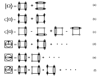
Figure 6: (a),(b) and (c) express the five bosonic states of the projected $SO(5)$ model in terms of the microscopic states on a plaquette. (d), (e) and (f) represent states with well-defined superspin directions, which can be obtained from the linear combinations of (a), (b) and (c). These states are analytically defined in Eq. (74) and Table II.

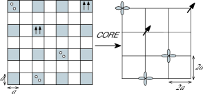
Figure 29: Illustration of the basic idea of the CORE method. To implement the CORE method, first decompose the original lattice in plaquettes, and then truncate the spectrum of a given plaquette to five lowest states, i.e, singlet, hole-pair and three magnon states. An effective Hamiltonian for these bosons can then be calculated using the CORE method. Left: local bosons in the original lattice. Gray rectangle denotes the singlet RVB vacua, circles denote holes and the set of two parallel vertical arrows denote the magnon. Right: local bosons on the lattice of plaquette. Leaf-like pattern denotes a local $d$-wave hole-pair on a plaquette. Canted arrow denotes local magnon on a plaquette. The singlet RVB vacuum is denoted by an empty site.

The $SO(5)$ quantum non-linear $\sigma$ model describes the kinetic and potential energies of coupled superspin degrees of freedom. In the case of HTSC cuprates, the superspin degrees of freedom are most conveniently defined on a coarse grained lattice, with $2a\times 2a$ lattice spacing in units of the original cuprate lattice spacing, where every super-site denotes a (non-overlapping) plaquette of the original lattice (see Fig. 29). There are $4^{4}=256$ states on a plaquette in the original Hubbard model, but we shall retain only the 6 lowest energy states, including a spin singlet state and three spin triplet states at half-filling, and two paired states with two holes or two particles away from half-filling (see Fig. 6). In sections V.3 and V.4, we will show, with numerical calculations, that these are indeed the lowest energy states in each charge sector. Additionally, we will show explicitly that the local superspin degree of freedom discussed in this section can be constructed from these six low energy states. Proposing the $SO(5)$ quantum non-linear $\sigma$ model as the low energy effective model of the HTSC cuprates requires the following physical assumptions: 1) AF and SC and their quantum disordered states are the only competing degrees of freedom in the underdoped regime. 2) Fermionic degrees of freedom are mostly gapped below the pseudogap temperature. For a $d$-wave superconductor, there are also gapless fermion degrees of freedom at the gap nodes. However, they do not play a significant role in determining the phase diagram and collective modes of the system. Our approach is to solve the bosonic part of the model first, and then include gapless fermions self-consistently at a later stage Demler and Zhang (1999a); Altman and Auerbach (2002).

From Eqs. (34) and the discussions in sections III.1, we see that $L_{ab}$ and $n_{a}$ are conjugate degrees of freedom, very much similar to $[q,p]=i\hbar$ in quantum mechanics. This suggests that we can construct a Hamiltonian from these conjugate degrees of freedom. The Hamiltonian of the $SO(5)$ quantum non-linear $\sigma$ model takes the following form

$$H=\frac{1}{2\chi}\sum_{x,a<b}L_{ab}^{2}(x)+\frac{\rho}{2}\sum_{\langle x,x^{\prime}\rangle,a}n_{a}(x)n_{a}(x^{\prime})+\sum_{x,a<b}B_{ab}(x)L_{ab}(x)+\sum_{x}V(n(x)),$$ (53)

where the superspin $n_{a}$ vector field is subjected to the constraint

$$n_{a}^{2}=1.$$ (54)

This Hamiltonian is quantized by the canonical commutation relations (33) and (34). Here, the first term is the kinetic energy of the $SO(5)$ rotors, where $\chi$ has the physical interpretation of the moment of inertia of the $SO(5)$ rotors. The second term describes the coupling of the $SO(5)$ rotors on different sites through the generalized stiffness $\rho$. The third term introduces the coupling of external fields to the symmetry generators, while $V(n)$ includes anisotropic terms which break the $SO(5)$ symmetry to the conventional $SO(3)\times U(1)$ symmetry. The $SO(5)$ quantum non-linear $\sigma$ model is a natural combination of the $SO(3)$ non-linear $\sigma$ model describing the AF Heisenberg model and the quantum XY model describing the SC to insulator transition. If we restrict the superspin to have only components $a=2,3,4$, then the first two terms describe the symmetric Heisenberg model, the third term describes the coupling to a uniform external magnetic field, while the last term can represent easy plane or easy axis anisotropy of the Neel vector. On the other hand, for $a=1,5$, the first term describes Coulomb or capacitance energy, the second term is the Josephson coupling energy, while the third term describes coupling to an external chemical potential.

The first two terms of the $SO(5)$ model describe the competition between the quantum disorder and classical order. In the ordered state, the last two terms describe the competition between the AF and SC order. Let us first consider the quantum competition. The first term prefers sharp eigenstates of the angular momentum. On an isolated site, $C\equiv\sum L_{ab}^{2}$ is the Casimir operator of the $SO(5)$ group in the sense that it commutes with all the $SO(5)$ generators. The eigenvalues of this operator can be determined completely from group theory - they are 0, 4, 6 and 10, respectively, for the 1 dimensional $SO(5)$ singlet, 5 dimensional $SO(5)$ vector, 10 dimensional antisymmetric tensor and 14 dimensional symmetric, traceless tensors, respectively. Therefore, we see that this term always prefers a quantum disordered $SO(5)$ singlet ground state, which is also a total spin singlet. In the case where the effective quantum non-linear $\sigma$ model is constructed by grouping the sites into plaquettes, the quantum disordered ground state corresponds to a plaquette “RVB” state, as depicted in Figs. 6a and 12a. This ground state is separated from the first excited state, the five fold $SO(5)$ vector state, by an energy gap of $2/\chi$. This gap will be reduced when the different $SO(5)$ rotors are coupled to each other by the second term. This term represents the effect of stiffness, which prefers a fixed direction of the $n_{a}$ vector to a fixed angular momentum. This competition is an appropriate generalization of the competition between the number sharp and phase sharp states in a superconductor and the competition between the classical Neel state and the bond or plaquette singlet state in the Heisenberg AF. The quantum phase transition occurs near $\chi\rho\simeq 1$.

In the classically ordered state, the last two anisotropy terms compete to select a ground state. To simplify the discussion, we first consider the following simple form of the static anisotropy potential:

$$V(n)=-g(n_{2}^{2}+n_{3}^{2}+n_{4}^{2}).$$ (55)

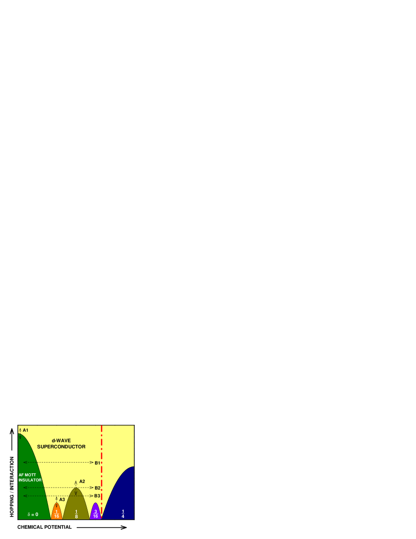
Figure 13: A typical global phase diagram of the extended $SO(5)$ model in the parameter space of chemical potential and the ratio of boson hopping energy over interaction energy (see Ref. Chen et al. (2003a) for details). This phase diagram shows self-similarity among the insulating states at half-filling and other rational filling fractions. There are two types of superfluid-insulator transition. The quantum phase transition of “class A” can be approached by varying the hopping energy, for example, by applying a pressure and magnetic field at constant doping. The quantum phase transition of “class B” can be realized by changing the chemical potential or doping. This theoretical phase diagram can be compared with the global phase diagram of the HTSC cuprates. Different families of cuprates correspond to different traces of “class B.” For example, we believe $YBCO$ is $B1$-like, $BSCO$ may be close to $B2$-like and $LSCO$ is $B3$-like. The vertical dash-dot line denotes a boundary in the overdoped region beyond which our pure bosonic model becomes less accurate. All the phase boundaries in this figure can be classified into direct first order (type 1), two second order (type 2), or a marginal case with enhanced symmetry (type 1.5). Type 2 transitions between CDW lobes and the superconducting state lead to intermediate supersolid phases.

At the particle-hole symmetric point with vanishing chemical potential $B_{15}=\mu=0$, the AF ground state is selected by $g>0$, while the SC ground state is selected by $g<0$. $g=0$ is the quantum phase transition point separating the two ordered phases. This phase transition belongs to “class $A$” in the classification scheme of section II and is depicted as the “$A1$” transition line in Fig. 13. This point has the full quantum $SO(5)$ symmetry in the model described above.

However, it is unlikely that the HTSC cuprates can be close to this quantum phase transition point. In fact, we expect the anisotropy term $g$ to be large and positive, making the AF phase strongly favored over the SC phase at half-filling. However, the chemical potential term has the opposite, competing effect and favors SC. We can observe this by transforming the Hamiltonian into the Lagrangian density in the continuum limit:

$${\cal L}=\frac{\chi}{2}\omega_{ab}(x,t)^{2}+\frac{\rho}{2}(\partial_{k}n^{a}(x,t))^{2}-V(n(x,t)),$$ (56)

where

$$\omega_{ab}=n_{a}(\partial_{t}n_{b}-iB_{bc}n_{c})-(a\leftrightarrow b)$$ (57)

is the angular velocity. We see that the chemical potential enters the Lagrangian as a gauge coupling in the time direction. Expanding the first term in the presence of the chemical potential $\mu=B_{15}$, we obtain an effective potential

$$V_{eff}(n)=V(n)-\frac{(2\mu)^{2}\chi}{2}(n_{1}^{2}+n_{5}^{2}),$$ (58)

from which we see that the bare $V$ term competes with the chemical potential term. For $\mu<\mu_{c}=\sqrt{g/\chi}$, the AF ground state is selected, while for $\mu>\mu_{c}$, the SC ground state is realized. At the transition point – even though each term strongly breaks $SO(5)$ symmetry – the combined term gives an effective static potential which is $SO(5)$ symmetric, as we can see from (58). This quantum phase transition belongs to “class $B$” in the classification scheme of section II. A typical transition of this type is depicted as the “$B1$” transition line in Fig. 13. Even though the static potential is $SO(5)$ symmetric, the full quantum dynamics is not. This can be seen most easily from the time dependent term in the Lagrangian. When we expand out the square, the term quadratic in $\mu$ enters the effective static potential in Eq. (58). However, there is also a $\mu$-dependent term involving a first order time derivative. This term breaks the particle hole symmetry and dominates over the second order time derivative term in the $n_{1}$ and $n_{5}$ variables. In the absence of an external magnetic field, only second order time derivative terms of $n_{2,3,4}$ enter the Lagrangian. Therefore, while the chemical potential term compensates the anisotropy potential in Eq. (58) to arrive at an $SO(5)$ symmetric static potential, its time dependent part breaks the full quantum $SO(5)$ symmetry. This observation leads to the concept of the projected or static $SO(5)$ symmetry. A model with projected or static $SO(5)$ symmetry is described by a quantum effective Lagrangian of the form

$${\cal L}=\frac{\chi}{2}\sum_{\alpha=2,3,4}(\partial_{t}n_{\alpha})^{2}-\chi\mu(n_{1}\partial_{t}n_{5}-n_{5}\partial_{t}n_{1})-V_{eff}(n),$$ (59)

where the static potential $V_{eff}$ is $SO(5)$ symmetric.

We see that “class $A$” transition from AF to SC occurs at a particle hole symmetric point, and it can have a full quantum $SO(5)$ symmetry. The “class $B$” transition from AF to SC is induced by a chemical potential; only static $SO(5)$ symmetry can be realized at the transition point. The “class $A$” transition can occur at half-filling in organic superconductors, where the charge gap at half-filling is comparable to the spin exchange energy. In this system, the AF to SC transition is tuned by pressure, where the doping level and the chemical potential stay fixed. The transition from the half-filled AF state to the SC state in the HTSC cuprates is far from the “class $A$” transition point, but static $SO(5)$ symmetry can be realized at the chemical potential induced transition. However, as we shall see in section IV.2, there are also Mott insulating states with AF order at fractional filling factors, for instance, at doping level $x=1/8$. The insulating gap is much smaller at these fractional Mott phases, and there is an effective particle-hole symmetry near the tip of the Mott lobes. For these reasons, “class $A$” transition with the full quantum $SO(5)$ symmetry can be realized again near the tip of fractional Mott phases, as in organic superconductors. Transitions near the fractional Mott insulating lobes are depicted as the “$A2$” and “$B2$” transitions in the global phase diagram (see Fig. 13). In this case, a transition from a fractional Mott insulating phase with AF order to the SC state can again be tuned by pressure without changing the density or the chemical potential.

The $SO(5)$ quantum nonlinear $\sigma$ model is constructed from two canonically conjugate field operators $L_{ab}$ and $n_{a}$. In fact, there is a kinematic constraint among these field operators. In the case of the Heisenberg model, the total spin operator and the AF Neel order parameter satisfy an orthogonality constraint, as expressed in Eq. (15). The $SO(5)$ generalization of this constraint can be expressed as follows:

$$L_{ab}n_{c}+L_{bc}n_{a}+L_{ca}n_{b}=0.$$ (60)

This identity is valid for any triples $a$, $b$ and $c$, and can be easily proven by expressing $L_{ab}=n_{a}p_{b}-n_{b}p_{a}$, where $p_{a}$ is the conjugate momentum of $n_{a}$. Geometrically, this identity expresses the fact that $L_{ab}$ generates a rotation of the $n_{a}$ vector. The infinitesimal rotation vector lies on the tangent plane of the four sphere $S^{4}$, as defined by Eq. (54), and is therefore orthogonal to the $n_{a}$ vector itself. Extending this geometric proof, WegnerWegner (2000) has shown that the $SO(5)$ orthogonality relation also follows physically from maximizing the entropy. Taking the triple $a,b,c$ to be $2,3,4$, and recognizing that $L_{\alpha\beta}=\epsilon_{\alpha\beta\gamma}S_{\gamma}$, this identity reduces to the $SO(3)$ orthogonality relation in Eq. (15). This $SO(5)$ identity places a powerful constraint on the expectation values of various operators. In particular, it quantitatively predicts the value of the $\pi$ order parameter in a mixed state between AF or SC. For example, let’s take the $a,b,c$ triple to be $1,2,5$. Eq. (60) predicts that

$$L_{15}n_{2}+L_{52}n_{1}+L_{21}n_{5}=0\ \ \Rightarrow\ \ \langle L_{25}\rangle=\langle Im\pi_{x}\rangle=\frac{Q\langle n_{2}\rangle}{\langle n_{1}\rangle},$$ (61)

where we chose the SC phase such that $\langle n_{5}\rangle=0$. Here, $Q=\langle L_{15}\rangle$ measures the hole density. Since these four expectation values can easily be measured numerically and, in principle, experimentally, this relationship can be tested quantitatively. Recently, Ghosal, Kallin and BerlinskyGhosal et al. (2002) tested this relationship within microscopic models of the AF vortex core. In this case, AF and SC coexist in a finite region near the vortex core, so that both $\langle n_{1}\rangle$ and $\langle n_{5}\rangle$ are non-vanishing. They found that the $SO(5)$ orthogonality constraint is accurately satisfied in microscopic models.

In this section, we presented the $SO(5)$ quantum non-linear $\sigma$ model as a heuristic and phenomenological model. The key ingredients of the model are introduced by observing the robust features of the phase diagram and the low energy collective modes of the HTSC cuprate system. This is the “top-down” approach discussed in the introduction. In this sense, the model has a general validity beyond the underlying microscopic physics. However, it is also useful to derive such a model directly from microscopic electronic models. Fortunately, this “bottom-up” approach agrees with the phenomenological approach to a large extent. A rigorous derivation of this quantum non-linear $\sigma$ model from an $SO(5)$ symmetric microscopic model on a bi-layer system will be given in section V.1, while an approximate derivation from the “realistic” microscopic $t-J$ and Hubbard model will be given in section V.4.

III.3 The projected SO(5) model with lattice bosons

In the previous section, we presented the formulation of the $SO(5)$ quantum nonlinear $\sigma$ model. This model is formulated in terms of two sets of canonically conjugate variables - the superspin vector $n_{a}$ and the angular momentum $L_{ab}$. The two terms which break the full quantum $SO(5)$ symmetry are the anisotropy term, $g$, and the chemical potential term, $\mu$. Therefore, this model contains high energy modes, particularly excitations of the order of the Mott insulating gap at half-filling. For this reason, GreiterGreiter (1997) and Baskaran and AndersonBaskaran and Anderson (1998) questioned whether the effective $SO(5)$ symmetry can be implemented in the low energy theory. In the previous section, it was shown that these two symmetry breaking terms could cancel each other in the static potential and the resulting effective potential could still be $SO(5)$ symmetric. It was also pointed out that the chemical potential term breaks the $SO(5)$ symmetry in the dynamic or time-dependent part of the effective Lagrangian. In response to these observations, Zhang et al. constructed the projected $SO(5)$ modelsZhang et al. (1999), which fully project out the high energy modes, and obtained a low energy effective quantum Hamiltonian, with an approximately $SO(5)$ symmetric static potential.

The first step is to perform a transformation from the $n_{a}$ and $L_{ab}$ coordinates to a set of bosonic operators. We first express the angular momentum operator as

$$L_{ab}=n_{a}p_{b}-n_{b}p_{a},$$ (62)

where $p_{a}$ is the canonical momentum conjugate to $n_{a}$, satisfying the Heisenberg commutation relation:

$$[n_{a},p_{b}]=i\delta_{ab}.$$ (63)

Furthermore, we can express the canonical coordinates and momenta in terms of the boson operators as

$$n_{a}=\frac{1}{\sqrt{2}}(t_{a}+t_{a}^{\dagger})\ \ \ p_{a}=\frac{1}{i\sqrt{2}}(t_{a}-t_{a}^{\dagger}),$$ (64)

where the boson operators satisfy the commutation relation

$$[t_{a},t_{b}^{\dagger}]=\delta_{ab},$$ (65)

and the (half-filled) ground state is defined by $t_{a}|\Omega\rangle=0$. There are five boson operators, $t_{\alpha}=t_{2},t_{3},t_{4}$ are the boson operators for the magnetic triplet excitations, also called the magnons, while

$$t_{1}=\frac{1}{\sqrt{2}}(t_{h}+t_{p})\ \ \ t_{5}=\frac{1}{i\sqrt{2}}(t_{h}-t_{p})$$ (66)

are the linear combinations of the particle pair ($t_{p}$) and hole pair ($t_{h}$) annihilation operators. In the $SO(5)$ quantum non-linear $\sigma$ model formulation, there is an infinite number of bosonic states per site. However, due to the first term in Eq. (53) (the angular momentum term), states with higher angular momenta or, equivalently, higher boson number, are separated by higher energies. Therefore, as far as the low energy physics is concerned, we can restrict ourselves to the manifold of six states per site, namely the ground state $|\Omega\rangle$ and the five bosonic states $t^{\dagger}_{a}|\Omega\rangle$. This restriction is called the hard-core boson constraint and can be implemented by the condition $t^{\dagger}_{a}t^{\dagger}_{b}|\Omega\rangle=0$. Within the Hilbert space of hard-core bosons, the original $SO(5)$ quantum non-linear $\sigma$ model is mapped onto the following hard-core boson model:

$$H = \Delta_{s}\sum_{x,\alpha=2,3,4}t_{\alpha}^{\dagger}t_{\alpha}(x)+\Delta_{c}\sum_{x,i=1,5}t_{i}^{\dagger}t_{i}(x)+\mu\sum_{x}(t_{p}^{\dagger}t_{p}(x)-t_{h}^{\dagger}t_{h}(x))$$ (67)

$$- J_{s}\sum_{\langle xx^{\prime}\rangle}n_{\alpha}(x)n_{\alpha}(x^{\prime})-J_{c}\sum_{\langle xx^{\prime}\rangle}n_{i}(x)n_{i}(x^{\prime}),$$

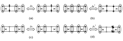
Figure 4: Illustration of hopping processes of the magnons and the hole pairs on a ladder. The cross denotes the center of a plaquette. An ellipse enclosing two sites denotes a spin singlet. (a) $J_{s}$ describes the magnon hopping, (b) $J^{\prime}_{s}$ describes the spontaneous creation and annihilation of a magnon pair. (c) $J_{c}$ describes the hopping of a hole pair, (d) $J^{\prime}_{c}$ describes the spontaneous creation and annihilation of a hole pair and a particle pair. In the full $SO(5)$ model, $J_{s}=J^{\prime}_{s}$ and $J_{c}=J^{\prime}_{c}$. In the projected $SO(5)$ model, the particle pair states are removed and $J^{\prime}_{c}=0$.

where $\Delta_{c}=2/\chi-2\mu^{2}\chi$ and $\Delta_{s}=2/\chi-g$ are the creation energies for the charge pairs and the triplet magnons, $\mu$ is the chemical potential, and $J_{c}$ and $J_{s}$ are the exchange energies for SC and AF, respectively. In the isotropic case, they are taken to be $\rho$ in the second term of Eq. (53). Expressing $n_{i}$ and $n_{\alpha}$ in terms of the bosonic operators, we see that the $J_{c}$ and $J_{s}$ terms describe not only the hopping, but also the spontaneous creation and annihilation of the charge pairs and the magnons, as depicted in Fig.4.

When $\Delta_{c}=\Delta_{s}$, $J_{c}=J_{s}$ and $\mu=0$, the model (67) has an exact quantum $SO(5)$ symmetry. In this case, the energy to create charge excitations is the same as the energy to create spin excitations. This situation could be realized in organic and heavy fermion superconductors near the AF phase boundary or the HTSC near commensurate doping fractions such as $x=1/8$, as we shall see in section IV.2. However, for HTSC systems near half-filling, the energy to create charge excitations is much greater than the energy to create spin excitations, ı.e. $\Delta_{c}\gg\Delta_{s}$. In this case, the full quantum $SO(5)$ symmetry is broken but, remarkably, the effective static potential can still be $SO(5)$ symmetric. This was seen in the previous section by the cancellation of the anisotropy potential $g$ term by the chemical potential $\mu$ term. In a hard-core boson model (67) with $\Delta_{c}\gg\Delta_{s}$, a low energy effective model can be derived by retaining only the hole pair state while projecting out the particle pair state. This can be done by imposing the constraint

$$t^{\dagger}_{p}(x)|\Omega\rangle=0$$ (68)

at every site $x$. The projected Hamiltonian takes the form

$$H = \Delta_{s}\sum_{x}t_{\alpha}^{\dagger}t_{\alpha}(x)+\tilde{\Delta}_{c}\sum_{x}t^{\dagger}_{h}t_{h}(x)$$ (69)

$$- J_{s}\sum_{\langle xx^{\prime}\rangle}n_{\alpha}(x)n_{\alpha}(x^{\prime})-J_{c}\sum_{\langle xx^{\prime}\rangle}n_{i}(x)n_{i}(x^{\prime}),$$

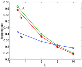
Figure 31: Boson hopping energies versus Hubbard $U$. The intersection region near $U=8$ is close to the projected $SO(5)$ symmetry point. All energies are in units of $t$.

where $\tilde{\Delta}_{c}=\Delta_{c}-\mu$. The Hamiltonian (69) has no parameters of the order of $U$. To achieve the static $SO(5)$ symmetry, we need $\Delta_{s}\sim\tilde{\Delta}_{c}$ and $J_{s}\sim J_{c}$. The first condition can always be met by changing the chemical potential, whereas the second one requires certain fine tuning. However, as we discuss in Section VD (see Fig. 31), this condition emerges naturally when one derives the model (69) from the Hubbard model in the relevant regime of parameters.

The form of the projected $SO(5)$ Hamiltonian hardly changes from the unprojected model (67), but the definition of $n_{1}$ and $n_{5}$ is changed from

$$n_{1} = \frac{1}{\sqrt{2}}(t_{1}+t_{1}^{\dagger})=\frac{1}{2}(t_{h}+t_{p}+t_{h}^{\dagger}+t_{p}^{\dagger})$$

$$n_{5} = \frac{1}{\sqrt{2}}(t_{5}+t_{5}^{\dagger})=\frac{1}{2i}(t_{h}-t_{p}-t_{h}^{\dagger}+t_{p}^{\dagger})$$ (70)

to

$$n_{1}=\frac{1}{2}(t_{h}+t_{h}^{\dagger})\ \ \ n_{5}=\frac{1}{2i}(t_{h}-t_{h}^{\dagger}).$$ (71)

From Eq. (70), we see that $n_{1}$ and $n_{5}$ commute with each other before the projection. However, after the projection, they acquire a nontrivial commutation relation, as can be seen from Eq. (71):

$$[n_{1},n_{5}]=i/2.$$ (72)

Therefore, projecting out doubly occupied sites, commonly referred to as the Gutzwiller projection, can be analytically implemented in the $SO(5)$ theory by retaining the form of the Hamiltonian and changing only the commutation relations.

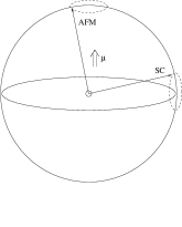
Figure 5: The chiral $SO(5)$ sphere has an $SO(5)$ symmetric shape but allows only one sense of the rotation in the SC plane $(n_{1},n_{5})$. Small oscillations around the equator, or the $\pi$ triplet resonance, are unaffected by the chiral projection. However, small oscillations around the north pole, or the $\pi$ doublet mode, are strongly affected: only one of the two such modes is retained after the projection.

The Gutzwiller projection implemented through the modified commutation relations between $n_{1}$ and $n_{5}$ is formally similar to the projection onto the lowest Landau level in the physics of the quantum Hall effect. For electrons moving in a 2D plane, the canonical description involves two coordinates, $X$ and $Y$, and two momenta, $P_{X}$ and $P_{Y}$. However, if the motion of the electron is fully confined in the lowest Landau level, the projected coordinate operators become non-commuting and are given by $[X,Y]=il_{0}^{2}$, where $l_{0}$ is the magnetic length. In the context of the projected $SO(5)$ Hamiltonian, the original rotors at a given site can be viewed as particles moving on a four dimensional sphere $S^{4}$, as defined by Eq. (54), embedded in a five dimensional Euclidean space. The angular momentum term $\frac{1}{2\chi}L_{ab}^{2}$ describes the kinetic motion of the particle on the sphere. The chemical potential acts as a fictitious magnetic field in the $(n_{1},n_{5})$ plane. In the Gutzwiller-Hubbard limit, where $\Delta_{c}\gg\Delta_{s}$, a large chemical potential term is required to reach the limit $\tilde{\Delta}_{c}\sim\Delta_{s}$. The particle motion in the $(n_{1},n_{5})$ plane becomes quantized in this limit, as in the case of the quantum Hall effect, and the non-commutativity of the coordinates $(n_{1},n_{5})$ given by Eq. (72) arises as a result of the projection. The projection does not affect the symmetry of the sphere on which the particle is moving; however, it restricts the sense of the kinetic motion to be chiral, i.e., only along one direction in the $(n_{1},n_{5})$ plane. (See Fig. 5). In this sense, the particle is moving on a chiral $SO(5)$ symmetric sphere. The non-commutativity of the $(n_{1},n_{5})$ coordinates is equivalent to the effective Lagrangian (see Eq. (59) of section III.2) containing only the first order time derivative. In fact, from Eq. (59), we see that in this case the canonical momenta associated with the coordinates $n_{1}$ and $n_{5}$ are given by

$$p_{1}=\frac{\delta L}{\delta\dot{n}_{1}}=\chi\mu n_{5}\ \ ,\ \ p_{5}=\frac{\delta L}{\delta\dot{n}_{5}}=-\chi\mu n_{1}.$$ (73)

Applying the standard Heisenberg commutation relation for the conjugate pairs $(n_{1},p_{1})$, or $(n_{5},p_{5})$ gives exactly the quantization condition (72). Note that in Eq. (73) $\chi\mu$ plays the role of the Planck’s constant in quantum mechanics. We see that the projected $SO(5)$ Hamiltonian (69) subjected to the quantization condition (72) is fully equivalent to the effective Lagrangian Eq. (59), discussed in the last section.

Despite its apparent simplicity, the projected $SO(5)$ lattice model can describe many complex phases, most of which are seen in the HTSC cuprates. These different phases can be described in terms of different limits of a single variational wave function of the following product form:

$$|\Psi\rangle=\prod_{x}(\cos\theta(x)+\sin\theta(x)(m_{\alpha}(x)t^{\dagger}_{\alpha}(x)+\Delta(x)t^{\dagger}_{h}(x)))|\Omega\rangle.$$ (74)

where the variational parameters $m_{\alpha}(x)$ should be real, while $\Delta(x)$ is generally complex. The normalization of the wave function, $\langle\Psi|\Psi\rangle=1$, requires the variational parameters to satisfy

$$\sum_{\alpha}|m_{\alpha}(x)|^{2}+|\Delta(x)|^{2}=1.$$ (75)

Therefore, we can parameterize them as $|m_{\alpha}(x)|^{2}=cos^{2}\phi(x)$ and $|\Delta(x)|^{2}=sin^{2}\phi(x)$, which is similar to the $SO(5)$ constraint introduced in Eq. (54). The expectation values of the order parameters and the symmetry generators in this variational state are given by

$$\langle\Psi|n_{\alpha}(x)|\Psi\rangle = \frac{1}{\sqrt{2}}sin2\theta(x)Re(m_{\alpha}(x))$$

$$\langle\Psi|n_{1}(x)|\Psi\rangle = \frac{1}{2}sin2\theta(x)Re(\Delta(x))$$

$$\langle\Psi|n_{5}(x)|\Psi\rangle = \frac{1}{2}sin2\theta(x)Im(\Delta(x))$$ (76)

and

$$\langle\Psi|Q(x)|\Psi\rangle = \langle\Psi t^{\dagger}_{h}(x)t_{h}(x)|\Psi\rangle=\sin^{2}\theta(x)~{}|\Delta(x)|^{2}$$

$$\langle\Psi|S_{\alpha}|\Psi\rangle = -\langle\Psi|i\epsilon^{\alpha\beta\gamma}t^{\dagger}_{\beta}(x)t_{\gamma}(x)|\Psi\rangle=-i\epsilon^{\alpha\beta\gamma}\sin^{2}\theta~{}m^{*}_{\beta}(x)m_{\gamma}(x)$$

$$\langle\Psi|\pi_{\alpha}(x)|\Psi\rangle = \langle\Psi|\frac{t^{\dagger}_{\alpha}(x)t_{h}(x)}{i\sqrt{2}}|\Psi\rangle=\frac{\sin^{2}\theta~{}m^{*}_{\alpha}(x)\Delta(x)}{i\sqrt{2}}.$$ (77)

Initially, we restrict our discussions to the case where the variational parameters are uniform, describing a translationally invariant state. Evaluating different physical operators in this state gives the result summarized in the following table:

		charge Q	spin S	AF order $\langle n_{\alpha}\rangle$	SC order $\langle n_{i}\rangle$	$\pi$ order $\langle\pi_{\alpha}\rangle$
(a)	“RVB” state: $sin\theta=0$	0	0	0	0	0
(b)	Magnon state: $cos\theta=0$ and $sin\phi=0$	0	1	0	0	0
(c)	“Hole pair” state: $cos\theta=0$ and $cos\phi=0$	-2	0	0	0	0
(d)	AF state: $0<sin\theta<1$ and $sin\phi=0$	0	indefinite	$\neq 0$	0	0
(e)	SC state: $0<sin\theta<1$ and $cos\phi=0$	indefinite	0	0	$\neq 0$	0
(f)	Mixed AF/SC state: $0<sin\theta<1$ and $0<sin\phi<0$	indefinite	indefinite	$\neq 0$	$\neq 0$	$\neq 0$
	$\pi$ state: $cos\theta=0$ and $0<cos\phi<1$	indefinite	indefinite	0	0	$\neq 0$

Table 2: Physical properties of various plaquette states classified according to the $SO(5)$ order parameters and symmetry generators.

As we can see, this wave function not only describes classically ordered states with spontaneously broken symmetry, but also quantum disordered states which are eigenstates of spin and charge. Generally, $\Delta_{c}$ and $\Delta_{s}$ favor quantum disordered states, while $J_{c}$ and $J_{s}$ favor classically ordered states. Depending on the relative strength of these parameters, a rich phase diagram can be obtained.

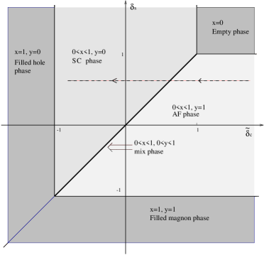
Figure 7: Phase diagram of the projected $SO(5)$ model (69) (for the case $J_{c}=2J_{s}\equiv J$) as a function of $\delta_{s}=\Delta_{S}/4J$ and $\tilde{\delta}_{c}=\tilde{\Delta}_{c}/4J$ . Variation of the chemical potential changes $\tilde{\Delta}_{c}$ and traces out a one-dimensional trajectory as shown on the dotted line. $x=sin^{2}\theta$ and $y=cos^{2}\phi$.

The phase diagram of the projected $SO(5)$ model with $J_{c}=2J_{s}\equiv J$ is shown in Fig. 7. Changing the chemical potential modifies $\tilde{\Delta}_{c}$ and traces out a one-dimensional path on the phase diagram. Along this path the system goes from the AF state to the uniform AF/SC mixed phase and then to the SC state. The mixed phase only corresponds to one point on this trajectory (i.e. a single value of the chemical potential $\mu_{c}$), although it covers a whole range of densities $0<\rho<\rho_{c}$. This suggests that the transition may be thought of as a first order transition between the AF and SC phases, with a jump in the density at $\mu_{c}$. The spectrum of collective excitations shown in Fig. 8, however, shows that this phase diagram also has important features of two second order phase transitions. The energy gap to $S=1$ excitations inside the SC phase vanishes when the chemical potential reaches the critical value $\mu_{c}$. Such a softening should not occur for the first order transition but is required for the continuous transition into a state with broken spin symmetry. This shows that models with the $SO(5)$ symmetry have intrinsic fine-tuning to be exactly at the border between a single first order transition and two second order transitions; in subsequent sections this type of transition shall be classified as type 1.5 transition. Further discussion of the phase diagram of the projected $SO(5)$ model is given in section VC. Note that effective bosonic Hamiltonians similar to (69) have also been considered in Refs. van Duin and Zaanen (2000); Park and Sachdev (2001).

IV THE GLOBAL PHASE DIAGRAM OF SO(5) MODELS

IV.1 Phase diagram of the classical model

The two robust ordered phases in the HTSC cuprates are the AF phase at half-filling and the SC phase away from half-filling. It is important to ask how these two phases are connected in the global phase diagram as different tuning parameters such as the temperature, the doping level, the external magnetic field, etc, one varied. Analyzing the $SO(5)$ quantum nonlinear $\sigma$ model, Zhang has classified four generic types of phase diagrams, presented as Fig. (1A)-(1D) in reference Zhang (1997). In the next section we are going to investigate the zero temperature phase diagram where the AF and the SC phases are connected by various quantum disordered states, often possessing charge order. In this section, we first focus on the simplest possibility, where AF and SC are the only two competing phases in the problem, and discuss the phase diagram in the plane of temperature and chemical potential, or doping level.

Let us first discuss the general properties of phase transition between two phases, each characterized by its own order parameter. In particular, we shall focus on the phenomenon of the enhanced symmetry at the multicritical point at which physically different static correlation functions show identical asymptotic behavior. In the case of CDW to SC transition discussed in section II, the CDW is characterized by an Ising like $Z_{2}$ order parameter, while the SC is characterized by a $U(1)$ order parameter. In the case of AF to SC transition, the order parameter symmetries are $SO(3)$ and $U(1)$, respectively. Generically, the phase transition between two ordered phases can be either a single direct first order transition or two second order phase transitions with a uniform mixed phase in between, where both order parameters are non-zero. This situation can be understood easily by describing the competition in terms of a LG functional of two competing order parametersKosterlitz et al. (1976), which is given by

$$F=r_{1}\phi_{1}^{2}+r_{2}\phi_{2}^{2}+u_{1}\phi_{1}^{4}+u_{2}\phi_{2}^{4}+2u_{12}\phi_{1}^{2}\phi_{2}^{2}.$$ (78)

Here, $\phi_{1}$ and $\phi_{2}$ are vector order parameters with $N_{1}$ and $N_{2}$ components, respectively. In the case of current interest, $N_{1}=2$ and $N_{2}=3$ and we can view $\phi^{2}_{1}=n_{1}^{2}+n_{5}^{2}$ as the SC component of the superspin vector, and $\phi^{2}_{2}=n_{2}^{2}+n_{3}^{2}+n_{4}^{2}$ as the AF component of the superspin vector. These order parameters are determined by minimizing the free energy $F$, and are given by the solutions of

$$2u_{1}\phi_{1}^{2}+2u_{12}\phi_{2}^{2}+r_{1}=0\ \ ,\ \ 2u_{12}\phi_{1}^{2}+2u_{2}\phi_{2}^{2}+r_{2}=0.$$ (79)

These equations determine the order parameters uniquely, except in the case when the determinant of the linear equations vanishes. At the point when

$$u_{1}u_{2}=u_{12}^{2}$$ (80)

and

$$\frac{r_{1}}{\sqrt{u_{1}}}=\frac{r_{2}}{\sqrt{u_{2}}},$$ (81)

the order parameters satisfy the relations

$$\frac{\phi^{2}_{1}}{\sqrt{u_{2}}}+\frac{\phi^{2}_{2}}{\sqrt{u_{1}}}=const,$$ (82)

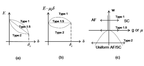
Figure 9: The energy (a) and the free energy (b) can depend on the density of a uniform AF/SC mixed state with a negative curvature when $u_{12}>\sqrt{u_{1}u_{2}}$, (classified as “type 1”) or a positive curvature when $u_{12}<\sqrt{u_{1}u_{2}}$ (classified as “type 2”). The $SO(5)$ symmetric limiting case of zero curvature, classified as “type 1.5,” is realized when $u_{12}=\sqrt{u_{1}u_{2}}$. (c) The “type 1” phase transition from the AF to SC state is a direct first order transition. There are two second order transitions from the AF to SC state in the “type 2” case. $SO(5)$ symmetry is realized at the intermediate case of “type 1.5.”

but they are not individually determined. In fact, with the re-scaling $\tilde{\phi}^{2}_{1}=\phi^{2}_{1}/\sqrt{u_{2}}$ and $\tilde{\phi}^{2}_{2}=\phi^{2}_{2}/\sqrt{u_{1}}$, the free energy is exactly $SO(5)$ symmetric with respect to the scaled variables, and Eq. (82) becomes identical to Eq. (54) in the $SO(5)$ case. Since the free energy only depends on the combination $\tilde{\phi}^{1}_{2}+\tilde{\phi}^{2}_{2}$, one order parameter can be smoothly rotated into the other without any energy cost. Equation (80) is the most important condition for the enhanced symmetry. We shall discuss extensively in this paper whether this condition is satisfied microscopically or close to some multi-critical points in the HTSC cuprates. On the other hand, equation (81) can always be tuned. In the case of AF to SC transition, the chemical potential couples to the square of the SC order parameter, as we can see from Eq. (58). Therefore, $r_{1}$ can be tuned by the chemical potential, and equation (81) defines the critical value of the chemical potential $\mu_{c}$ at which the phase transition between AF and SC occurs. At this point, the chemical potential is held fixed, but the SC order parameter and the charge density can change continuously according to Eq. (82). Since the free energy is independent of the density at this point, the energy, which differs from the grand canonical free energy by a chemical potential term $\mu\delta$, can depend only linearly on the density. The linear dependence of the energy on doping is a very special, limiting case. Generally, the energy versus doping curve would either have a negative curvature, classified as “type 1,” or a positive curvature, classified as “type 2” (see Fig. 9a). The special limiting case of “type 1.5” with zero curvature is only realized at the $SO(5)$ symmetric point. The linear dependence of the ground state energy of a uniform AF/SC mixed state on the density is a crucial test of the $SO(5)$ symmetry which can be performed numerically, as we shall see in section V.2 and V.3. The constancy of the chemical potential and the constancy of the length of the $SO(5)$ superspin vector (82) as a function of density can be tested experimentally as well, as we shall discuss in section V.2.

The constancy of the chemical potential as a function of the density in a uniform system is a very special situation which only follows from the enhanced symmetry at the phase transition point. In a system with phase separation, the chemical potential is also independent of the total density, but the local density is non-uniform. The two phases are generally separated by a domain wall. The $SO(5)$ symmetric case can be obtained from the phase separation case in the limit where the width of the domain wall goes to infinity and a uniform state is obtained. This situation can be studied analytically by solving Eq. (79). Defining the parameters that characterize the deviation from the symmetric point as $w=u_{12}-\sqrt{u_{1}u_{2}}$ and $g=(\frac{r_{1}}{\sqrt{u_{1}}}-\frac{r_{2}}{\sqrt{u_{2}}})/2$, it is obvious that the phase transition between the two forms of order is tuned by $g$, while $w$ determines the nature of the phase transition. The phase diagram in the $(g,w)$ plane is shown in Fig. 9c. For $w>0$, the two ordered phases are separated by a first order line. This type of transition is classified as “type 1.” On the other hand, when $w<0$, the two ordered phases are separated by two second order phase transition lines with an intermediate mixed phase where two orders coexist, i.e. $\langle\phi_{1}\rangle\neq 0$ and $\langle\phi_{2}\rangle\neq 0$. This type of transition is classified as “type 2.” The limiting “type 1.5” behavior corresponds to the symmetric point $w=0$. Approaching this point from $w>0$, the first order transition becomes weaker and weaker and the latent heat associated with the first order transition becomes smaller and smaller. Therefore, the symmetric point can be viewed as the end point of a first order transition. On the other hand, approaching the symmetric point from $w<0$, the width of the intermediate mix phase becomes smaller and smaller, until the two second order transition lines merge into a single transition at $w=0$. From the above discussion, we learn an important lesson: the phase transition between two ordered phases can be either a direct first order transition or two second order transitions with an intermediate mixed phase. Furthermore, the symmetric point realizes a limiting behavior which separates these two scenarios. Balents, Fisher and NayakBalents et al. (1998), Lee and KivelsonLee and Kivelson (2003) pointed out that the “type 1” and “type 2” transitions of a Mott insulator induced by varying the chemical potential is analogous to the two types of superconductor to normal state transitions induced by a magnetic field. The magnetic field induces a direct first order transition from the SC state to the normal state in “type 1” superconductors, while it induces two second order transitions with an intermediate mix state in the “type 2” superconductors. Indeed, the limiting “type 1.5” behavior separating the “type 1” and the “type 2” superconductors also has a special symmetry, where the Bogomol’nyi’s bound for the vortex is satisfied as an equality. We note that recent work of Senthil et al discussed an alternative scenario for a direct second order transition between two phases with different order parameters and without a higher symmetry at the transition point. This was achieved by having fractionalizated excitations at the quantum critical point Senthil et al. (2004).

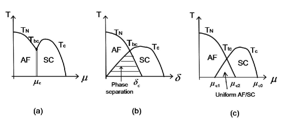
Figure 10: The finite temperature phase diagram in D=3 for the class “B1” transition shown in Fig. 13. (a) and (b), correspond to a direct first order phase transition between AF and SC, as a function of the chemical potential and doping, respectively. This type of transition is classified as the “type 1” transition. (c) corresponds to two second order phase transitions with a uniform AF/SC mix phase in between. This type of transition is classified as “type 2” transition. The AF and SC transition temperatures $T_{N}$ and $T_{c}$ merge into either a bi-critical $T_{bc}$ or a tetra-critical point $T_{tc}$.

Let us now turn to the finite temperature phase transitions. In $D=3$, finite temperature phase transitions associated with continuous symmetry breaking are possible. Therefore, the order parameters $\phi_{1}$ and $\phi_{2}$ can each have their own phase transition temperature, $T_{c}$ and $T_{N}$. The interesting question is how these two second order lines merge as one changes the parameter $g$ or, equivalently, the chemical potential $\mu$, which interchanges the relative stability of the two ordered phases. There are two generic possibilities. The “type 1” phase diagram is shown in Fig. 10a, where the two second order phase transition lines intersect at a bi-critical point, $T_{bc}$, which is also the termination point of the first order transition line separating the two ordered phases. This type of phase diagram is realized for $u_{12}>\sqrt{u_{1}u_{2}}$. The first order transition at $\mu_{c}$ separates the AF and SC states with different densities; therefore, the $T$ versus $\delta$ phase diagram shown in Fig. 10b contains a region of phase separation extending over the doping range $0<\delta<\delta_{c}$. The “type 2” phase diagram is shown in Fig. 10c, where $T_{c}$ and $T_{N}$ intersect at a tetra-critical point, below which a uniform AF/SC mixed phase separates the two pure phases by two second order transition lines. This type of phase diagram is realized for $u_{12}<\sqrt{u_{1}u_{2}}$.

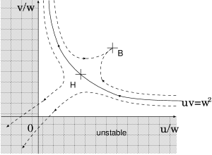
Figure 11: Renormalization group flow in the $(u_{1}/u_{12},u_{2}/u_{12})$ plane. (In this figure, $u=u_{1}$, $v=u_{2}$ and $w=u_{12}$.) The renormalization group flow is initially attracted towards the symmetric Heisenberg point labelled by H. The RG trajectories diverge near the Heisenberg model, with a very small exponent. Reproduced from Ref. Murakami and Nagaosa (2000).

In contrast to the conventional superconductors with a long coherence length, the HTSC cuprates have a short coherence length and a large Ginzburg region. Thus, they have the possibility of observing non-trivial critical behaviors. An interesting point concerns the symmetry at the multi-critical point where $T_{N}$ and $T_{c}$ (or, more generally, $T_{1}$ and $T_{2}$) intersect. At the multi-critical point defined by $r_{1}=r_{2}=0$, the critical fluctuations of the order parameters couple to each other and renormalize the coefficients of the fourth order terms $u_{1}$, $u_{2}$ and $u_{12}$. There are several possible fixed points. The symmetric fixed point, also known as the Heisenberg fixed point, is characterized by $u^{*}_{1}=u^{*}_{2}=u^{*}_{12}$. The $O(N_{1})\times O(N_{2})$ symmetry is enhanced at this point to the higher $O(N_{1}+N_{2})$ symmetry. Another fixed point, called the biconical tetra-critical point in the literature, has non-vanishing values of $u_{1}^{*}$, $u_{2}^{*}$ and $u_{12}^{*}$ at the fixed point which deviates from the $O(N_{1}+N_{2})$ symmetry. The third possible fixed point is the decoupled fixed point, where $u_{12}^{*}=0$ and the two order parameters decouple from each other at the fixed point. The relative stability of these three fixed points can be studied analytically and numerically. The general picture is that there are two critical values, $N_{c}$ and $N_{c}^{\prime}$. For $N_{1}+N_{2}<N_{c}$, the symmetric bi-critical point is stable, for $N_{c}<N_{1}+N_{2}<N_{c}^{\prime}$, the biconical point is stable, while for $N_{1}+N_{2}>N_{c}^{\prime}$, the decoupled point becomes stable. The renormalization group calculations based on the $4-\epsilon$ expansionKosterlitz et al. (1976) places the value of $N_{c}$ close to 4 and the value of $N_{c}^{\prime}$ close to 11. The RG flow diagram is shown in Fig. 11 for the case of $N_{1}=3$ and $N_{2}=2$. Initially, all RG trajectories flow towards the symmetric fixed point. The manner in which the trajectories diverge close to the symmetric point depends on the values of the initial parameters. The trajectories flow to the symmetric point when $u_{12}^{2}=u_{1}u_{2}$, to the biconical point when $u_{12}^{2}<u_{1}u_{2}$, and flow outside of the regime of weak coupling RG analysis when $u_{12}^{2}>u_{1}u_{2}$. In the case of competition between AF and SC, $N=N_{1}+N_{2}=5$ is very close to $N_{c}$, leading to two important consequences. First, the biconical point breaks the $SO(5)$ symmetry weakly. The value of the interaction parameters at the biconical fixed point is given by $(u_{1}^{*};u_{2}^{*};u_{12}^{*})=2\pi^{2}\epsilon(0.0905;0.0847;0.0536)$. Extrapolating to $\epsilon=1$ gives the root mean square deviation from the symmetric $SO(5)$ point to about $26\%$, indicating weak $SO(5)$ symmetry breaking. The second consequence is that the critical exponent associated with the flow away from the symmetric, $SO(5)$ point is extremely slow. The first loop $4-\epsilon$ expansion gives the value of $1/13$ for the exponent associated with the flow away from the symmetric point. To get an estimate of the order of magnitude, we take the initial value of the scaling variable taking the flow away from the $SO(5)$ fixed point to be $0.04$. This value is obtained by considering the quantum corrections associated with a projected $SO(5)$ model Arrigoni and Hanke (2000). In this case, the significant deviation away from the symmetric point can only be observed when the reduced temperature is $t=(T-T_{bc})/T_{bc}\approx 10^{-11}$, making the departure away from the $SO(5)$ symmetric point practically unobservable. Indeed, numerical simulations of the $SO(5)$ models presented in section IV.3 are consistent with the $SO(5)$ symmetric behavior in a wide range of temperatures and in very large systems. However, it should be noted that they do not prove the ultimate stability of the symmetric point.

The question of the stability of the $SO(5)$ symmetric bicritical point has been raised and discussed extensively in literatureBurgess et al. (1998); Arrigoni and Hanke (2000); Murakami and Nagaosa (2000); Hu and Zhang (2000); Hu (2001); Aharony (2002); Jöstingmeier et al. (2003); Calabrese et al. (2003). Because the possible flow away from the bicritical point is extremely slow, experimental and numerical observation of the $SO(5)$ symmetric bi-critical behavior should be possible in a wide range of temperatures, if the starting microscopic parameters are already close to the symmetric point $u_{12}=\sqrt{u_{1}u_{2}}$. The $SO(5)$ symmetric bi-critical point has a distinct set of critical exponents, summarized in Ref. Hu and Zhang (2000), which can be distinguished experimentally from the usual $SO(3)$ and $U(1)$ behavior. In this sense, the experimental observation of the bi-critical behavior would demonstrate that the microscopic model of the HTSC cuprates is close to the $SO(5)$ symmetry. In section VII.4 we shall discuss the analysis of Murakami and NagaosaMurakami and Nagaosa (2000) showing bi-critical scaling behavior in the $\kappa$-BEDT organic superconductors. If the microscopic parameters are far from the the symmetric point $u_{12}=\sqrt{u_{1}u_{2}}$, other critical behaviors could be observed. AharonyAharony (2002) proposed the decoupled tetra-critical fixed point with $u^{*}_{12}=0$. As previously discussed , this critical point can be observed in experiments only if the microscopic value of $u^{*}_{12}$ is already close to zero (due to the extremely slow flows of parameters). For the HTSC cuprates, the AF vortex core experiments discussed in section VII.1 clearly show that the AF and SC order parameters are strongly and repulsively coupled with $u^{*}_{12}>0$. Therefore, the decoupled fixed point is unlikely to be relevant for these materials. However, this behavior could be realized in some heavy fermion systems where different bands are responsible for the AF and SC phases separately. Kivelson et alKivelson et al. (2001) and Calabrese et alCalabrese et al. (2003) also considered the possibility of tri-critical points, where some of the quartic terms $u_{1},u_{2},u_{12}$ become negative and the sixth order terms become important. In this case, the phase diagram could have topologies different from those listed here, and the readers are referred to the more extensive discussions given in Ref. Kivelson et al. (2001), especially Fig. 1c and 1d of that reference. Negative values of the quartic coefficient in the free energy (78) may come from the runaway flows shown in Fig. 11. A multi-critical point most closely related to the bi-critical point is the biconical tetra-critical point. Its relevance to the HTSC cuprates has been discussed in Ref.Zhang (1997); Zhang et al. (2002).

IV.2 Phase diagram of the quantum model

Having discussed the finite temperature phase diagram of the classical model, we now present the global phase diagram of the quantum model at zero temperature. The quantum phase transitions in the $SO(5)$ model were discussed in Fig. (1C) and (1D) in reference Zhang (1997). The quantum critical behavior of the $SO(5)$ models have also been studied extensively in Ref. Kopec and Zaleski (2001, 2003); Zalcski and Kopec (2000); Zaleski and Kopec (2000). This section extends the original analysis to include quantum disordered states with inhomogeneous charge distributions. The analysis carried out in this section is based on the bosonic projected $SO(5)$ model, which bears great similarities to the phase diagrams of the hardcore boson model studied extensively in Ref. Fisher et al. (1989); Bruder et al. (1993); Scalettar et al. (1995); vanOtterlo et al. (1995); Pich and Frey (1998); Hebert et al. (2002); Bernardet et al. (2002). The iterative construction of the global phase diagram of the $SO(5)$ model is also inspired by the global phase diagram of the quantum Hall effect constructed by Kivelson, Lee and ZhangKivelson et al. (1992).

The projected $SO(5)$ model given in Eq. (69) contains the creation energy and the hopping process of the magnons and hole pairs. The variational wave function for this model has the general form given in (74), with variational parameters $\theta(x)$, $m_{\alpha}(x)$ and $\Delta(x)=m_{1}(x)+im_{5}(x)$. The expectation value of the energy in this state is given by

$$\langle\Psi|H|\Psi\rangle=E(\theta(x),m_{a}(x))$$ (83)

$$= -\frac{J_{s}}{2}\sum_{xx^{\prime};\alpha=2,3,4}sin2\theta(x)sin2\theta(x^{\prime})m_{\alpha}(x)m_{\alpha}(x^{\prime})-\frac{J_{c}}{4}\sum_{xx^{\prime};i=1,5}sin2\theta(x)sin2\theta(x^{\prime})m_{i}(x)m_{i}(x^{\prime})$$

$$+\Delta_{s}\sum_{x;\alpha=2,3,4}\sin^{2}\theta(x)m_{\alpha}^{2}(x)+\tilde{\Delta}_{c}\sum_{x;i=1,5}\sin^{2}\theta(x)m_{i}^{2}(x).$$

The variational minimum is taken with respect to the normalization condition (75). In the regime when the quantum fluctuations are small, $\theta(x)$ can be taken to be fixed and uniform. In this case, the variational energy is nothing but the energy functional of a classical, generally anisotropic $SO(5)$ rotor model, which has been studied extensively numericallyHu (2001). At the point $J_{c}=2J_{s}$ and $\tilde{\Delta}_{c}=\Delta_{s}$ in parameter space, this rotor model is $SO(5)$ symmetric at the classical level. However, unlike the classical $SO(5)$ rotor, the projected $SO(5)$ model also contains quantum fluctuations and quantum disordered phases. The phase diagram of the projected $SO(5)$ model has been studied extensively by Quantum Monte Carlo simulationsChen et al. (2003a); Jöstingmeier et al. (2003); Dorneich et al. (2002b); Riera (2002a, b), and the results will be reviewed in details in section IV.3. When the quantum fluctuations are not strong enough to destroy classical order, the general topology of the phase diagram is similar to that classified in section IV.1.

In this section, we discuss the regime when quantum fluctuations are non-negligible and focus on the global phase diagram when the classical order competes with the quantum disorder and uniform states compete with non-uniform states. In Fig. 6 and table II, we see that the classically ordered states are obtained from the linear superpositions of quantum disordered states. The quantum disordered states are realized in the regime where the kinetic energy of the superspin $\Delta_{s}$ and $\Delta_{c}$ overwhelms the coupling energy of the superspin $J_{s}$ and $J_{c}$, and the superspin vector becomes disordered in the temporal domain. In this sense, the quantum description of the superspin goes far beyond the classical LG theory discussed in the previous section.

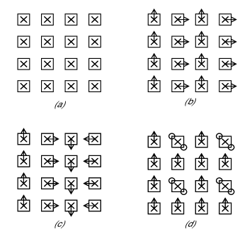
Figure 12: Some possible ground states of the projected $SO(5)$ model (see also Fig. 6). The cross depicts an RVB like spin singlet state on a plaquette, the arrow denotes the direction of the superspin, and the open circles depict hole pairs. (a) The plaquette RVB state is described by $\theta(x)=0$ on every plaquette. (b) The in-phase SC stripe with $\alpha(x)=0,\pi/2,0,\pi/2$ on each stripe. (c) The superspin spiral with $\alpha(x)=0,\pi/2,\pi,3\pi/2$ on each stripe. (d) The hole pair checkerboard state with $\alpha(x)=0$ everywhere, except on the hole pair plaquettes, where $\theta=\pi/2$ and $\alpha=\pi/2$.

By arranging the six elementary states from Fig. 6 into a spatially non-uniform patterns, we have infinitely many possibilities. In addition to the classically ordered AF and SC states, in Fig. 12 we illustrate some of the basic non-uniform states and their associated wave functions, expressed in terms of $\theta(x)$, $m_{\alpha}(x)$ and $\Delta(x)$. Stripe order was theoretically predicted and experimentally observed in the HTSC cupratesZaanen and Gunnarsson (1989); Tranquada et al. (1995); Kivelson et al. (1998); White and Scalapino (1998). In a typical stripe phase, a magnetic stripe of width $2a$ is separated by a charge stripe of width $2a$, where $a$ is the lattice constant. The stripe state come in two forms. For the in-phase stripes, both the charge and the spin periodicity is $4a$ in the direction transverse to the stripe direction. For the out-of-phase stripes, the charge periodicity is $4a$, while the spin periodicity is $8a$. The charge stripe can either be insulating, or superconducting. The SC stripes are defined by their phase angle; the two nearby SC stripes can be either in-phase or out-of-phase. The case when both the AF and the stripes are out of phase can be viewed as a superspin spiral, in which the superspin direction rotates continuously along the direction transverse to the stripes. (See Fig. 12c). Both types of stripes discussed here have both AF and SC orders. Another possibility is the checkerboard pair-density-wave (PDW)Chen et al. (2002), depicted in Fig. 12d. It can be obtained from the in-phase stripe by quantum disordering the hole pairs in the SC stripe. This state is insulating with AF and charge orders. We stress that all insulating states in the $SO(5)$ theory are obtained from the quantum disordered states of the hole pairs; therefore, they are paired insulators, in contrast to ordinary band insulators or a Wigner crystal state of the electrons.

Therefore, some of the inhomogeneous states observed in the HTSC cuprates can be described naturally in terms of the temporal and spatial ordering of the superspin. The key question is how they are energetically stabilized in the projected $SO(5)$ model. These spatially non-uniform states are usually realized when extended interactions are considered. These extended interactions take the form

$$H_{ext}=(V_{c}\sum_{\langle xx^{\prime}\rangle}+V^{\prime}_{c}\sum_{\langle\langle xx^{\prime}\rangle\rangle})n_{h}(x)n_{h}(x^{\prime})$$

$$+(V_{s}(S_{T})\sum_{\langle xx^{\prime}\rangle}+V^{\prime}_{s}(S_{T})\sum_{\langle\langle xx^{\prime}\rangle\rangle})\sum_{S_{T}=0,1,2}(t^{\dagger}(x)t^{\dagger}(x^{\prime}))_{S_{T}}(t(x)t(x^{\prime}))_{S_{T}}$$

$$+J_{\pi}\sum_{\langle xx^{\prime}\rangle}(t_{\alpha}^{\dagger}(x)t_{\alpha}(x^{\prime})t_{h}^{\dagger}(x^{\prime})t_{h}(x)+H.c.)+V_{\pi}\sum_{\langle xx^{\prime}\rangle}(n_{h}(x)n_{t}(x^{\prime})+n_{h}(x^{\prime})n_{t}(x))+...$$ (84)

Here $\langle xx^{\prime}\rangle$ and $\langle\langle xx^{\prime}\rangle\rangle$ denote the summation over the nearest-neighbor and the next-nearest-neighbor on a square lattice. $(t(x)t(x^{\prime}))_{S_{T}}$ refers to the total spin $S_{T}=0,1,2$ combinations of two magnons on sites $\langle xx^{\prime}\rangle$. The $V_{c}$ and $V^{\prime}_{c}$ terms describe the interaction of the hole pairs, the $V_{s}$ and $V^{\prime}_{s}$ terms describe the interaction of the magnons, and the $J_{\pi}$ and $V_{\pi}$ terms describe the mutual interaction of the hole pair and the magnon. Since the projected $SO(5)$ model is defined on a coarse-grained lattice, the density of the hole pairs, $n_{h}$, is related to the hole doping density by $n_{h}=2\delta$. The model Hamiltonian given by $H+H_{ext}$ has been studied extensively by Chen et alChen et al. (2003a) by using both quantum Monte Carlo methods and mean field theory. Here we summarize the basic qualitative results. In order to study the phase diagram of this model, we first focus on the charge sector. The charge sector of the projected $SO(5)$ model is the same as the hard-core boson model introduced in Eq. (16) of section II. This model has been much studied in the context of superfluid-to-insulator transitionBruder et al. (1993); Scalettar et al. (1995); vanOtterlo et al. (1995); Pich and Frey (1998); Hebert et al. (2002); Bernardet et al. (2002). Without the extended interactions $V(x,x^{\prime})$ in Eq. (12), the phase diagram of the hard-core boson is given in Fig. 3a. Half-filling of the original electron systems in the cuprates corresponds to the vacuum state of the hole-pairs, or phase III in Fig. 3a. The chemical potential $\mu$ induces a transition into the SC state, labelled as phase II. Further increase of the chemical potential induces a transition into a checker-board ordered state, labelled as phase I. This is the “class $B$” transition shown in Fig. 3a. Phase I corresponds to $n_{h}=1/2$ of the hole pair bosons, or $\delta=1/4$ of the original electrons. When extended interactions in $V(x,x^{\prime})$ are included, a new insulating phase develops near the overlapping region of phase I and phase III, with boson density of $n_{h}=1/4$ of the hole pair bosons, or $\delta=1/8$ of the original electrons (see, for instance, Fig. 2 of Ref. Bruder et al. (1993)). This insulating phase can have either stripe or checkerboard like charge order. Generally, stripe type of insulating order is favored for $V^{\prime}_{c}\gg V_{c}$, and the checkerboard-type order is favored in the opposite limitPich and Frey (1998); Hebert et al. (2002). With even more extended interactions, additional phases develop at lower rational densities. These Mott insulating phases at various rational densities are shown in Fig. 13. The phase boundary between the insulating phases with charge order and the SC phases can be generally classified into “type 1, 1.5 and 2,” according to the terminology developed in section IV.1 and Fig. 9. In the last two cases, a mixed phase, called the supersolid phase, develops near the phase boundary. After understanding the generic phase diagram of the hard-core lattice boson model, we are now in a position to discuss the full global phase diagram of the $SO(5)$ model $H+H_{ext}$, depicted in Fig. 13. Here $J/V$ denote the typical ratio of $J_{c}/V_{c}$, but it can obviously be replaced by other similar parameters. The $n_{h}=0$ phase corresponds to the AF state at half-filling, where magnons condense into the singlet ground state. For large values of $J/V$, a pure SC state is obtained where the hole pairs condense into the singlet ground state. However, besides these two robust, classically ordered phases, we also see new insulating phases at $n_{h}=1/4$, $n_{h}=1/8$ and $n_{h}=3/8$, which correspond to $\delta=1/8$, $\delta=1/16$ and $\delta=3/16$ in the real system. These new insulating states are stabilized by the extended interactions and have both AF and PDW order (see example Fig. 12d). As the chemical potential or the doping level is varied, a given system traces out a one dimensional slice in this phase diagram, with typical slices $B1$, $B2$ and $B3$ depicted in Fig. 13(we expect the quantum parameter $J/V$ to be independent of $\mu$ for a given family of materials). The nature of the phase transition $B1$ is similar to that of the classical model already discussed in section IV.1. In this case, the phase transition from the AF to SC state can be further classified into “types 1, 1.5 and 2,” as discussed in section IV.1, with the two latter cases leading to an AF/SC mixed phase at the phase transition boundary. For lower values of $J/V$, the trace $B3$ encounters the $\delta=1/8$ insulating phase. The key signature of this type of phase transition is that the SC $T_{c}$ will display a pronounced minimum as the doping variation traces through the $\delta=1/8$ insulating state. At the same time, the AF ordering (possibly at a wave vector shifted from $(\pi,\pi)$) will show reentrant behavior as doping is varied. The phase transition around the fractional insulating phases can again be classified into types “1, 1.5 and 2,” with possible AF/SC, AF/PDW, SC/PDW and AF/PDW/SC mix phases.

So far we have classified all quantum phase transitions in the $SO(5)$ models according to two broad classes. “Class $A$” describes transitions at a fixed chemical potential, typically at an effectively particle-hole symmetric point. “Class $B$” describes transitions in which the chemical potential or the density is varied. Each broad class is further classified into three “types, 1, 2 and 1.5,” depending on whether the transition is a direct first order, two second order, or an intermediate symmetric point in between. The full quantum $SO(5)$ symmetry can only be realized in the “class $A$ type 1.5” quantum phase transition. The Heisenberg point in the hard-core boson problem discussed in section II is one such example. The $g=0$ point in the $SO(5)$ quantum non-linear $\sigma$ model (53) is another example. On the other hand, the static, or projected $SO(5)$ symmetry can be realized in “class $B$ type 1.5” transitions. We believe that the AF to SC transitions in the YBCO, BCCO and NCCO systems correspond to “class $B1$” transition. These systems only have an AF to SC transition, which can be further classified as types “1, 1.5 and 2,” but they do not encounter additional statically ordered fractional insulating phases. On the other hand, the phase transition in the LSCO system, where $T_{c}$ displays a pronounced dip at $\delta=1/8$, corresponds to the “class B3” transition (see Fig. 13). In the HTSC cuprates, the charge gap at half-filling is very large, of the order of $U\sim 6eV$; it is not possible to induce the “class A1” transition from the AF to SC state by conventional means. However, the charge gap at the fractional insulating states is much smaller, of the order of $J$, and it is possible to induce the “class A2” insulator to superconductor transition by applying pressureLocquet et al. (1998); Sato et al. (2000); Arumugam et al. (2002); Takeshita et al. (2003). It would be interesting to determine if this transition point could have the full quantum $SO(5)$ symmetry.

Therefore, we see that the concept of the $SO(5)$ superspin indeed gives a simple and unified organizational principle to understand the rich phase diagram of the cuprates and other related systems. This construction of the global phase diagram can obviously be iterated ad infinitum to give a beautiful fractal structure of self-similar phases and phase transitions. All of this complexity can be simply reduced to the five elementary quantum states of the superspin.

IV.3 Numerical simulations of the classical and quantum models

In this section, we review essentially exact numerical studies of the classical $SO(5)$ model and the quantum projected $SO(5)$ model on a latticeChen et al. (2003a); Jöstingmeier et al. (2003); Dorneich et al. (2002b); Hu (1999b, 2001); Riera (2002a, b). In section V.4 we shall discuss the transformation from the microscopic models into the effective $SO(5)$ models and determine the effective parameters. Once this is accomplished, the phase diagram of the model can be determined reliably by bosonic QMC simulations. These calculations can be carried out for system sizes up to two orders of magnitude larger than fermionic QMC simulations, with the latter being plagued, in the physically interesting regime – i. e., close to half-filling – by the minus-sign problem der Linden (1992). The effective models can also be studied numerically in 3D; this is crucial, since there exists no AF ordered phase in 2D at finite temperature (nor long-range SC order). Thus, we are forced to study the 3D case in order to determine the phase diagram and to show that the scaling behavior is consistent with an $SO(5)$ symmetric critical behavior within the parameter regime studied (temperature and system size). This was possible due to a major step forward in the numerically accessible system sizes Sandvik (1997, 1999); Dorneich and Troyer (2001): in the bosonic projected $SO(5)$ model $\sim$10.000 sites were included, in contrast to just $\sim$100 sites in fermionic QMC calculations Dopf et al. (1992); Imada et al. (1998); Dagotto (1994). The numerical results, obtained by the QMC technique of Stochastic Series Expansion (SSE) Sandvik (1997, 1999) and reviewed here, show that the projected $SO(5)$ model can give a realistic description of the global phase diagram of the HTSC cuprates and accounts for many of their physical properties.

The form of the projected $SO(5)$ Hamiltonian is given in Eq. (69). The extended $SO(5)$ model also includes the interactions expressed in Eq. (84). We shall discuss the simple $SO(5)$ model first. In Ref. Zhang et al. (1999), this Hamiltonian was studied analytically within a mean-field approach. At the special point $J_{c}=2J_{s}\equiv J$ and $\Delta_{s}=\tilde{\Delta}_{c}$, the mean-field level of the ground-state energy of Hamiltonian ( 69) depends on the AF and SC order parameters $x=\langle t^{{\dagger}}_{x}\rangle$ and $y=\langle t^{{\dagger}}_{h}\rangle$ only via their combination $x^{2}+y^{2}$, which reflects the $SO(5)$ invariance of the mean-field approximation. In the full model, however, quantum fluctuations modify the zero-point energy of the bosons in Eq. ( 69); therefore, giving a correction to the ground-state energy which depends on $x$ and $y$ separately and destroys $SO(5)$ symmetry Zhang et al. (1999). Hence it is essential to study the full quantum-mechanical model (69), including all quantum fluctuations, which can only be done by means of numerical simulations. We then compare the properties of the projected $SO(5)$ model first in two dimensions (2D) with a variety of salient features of the HTSC such as the global phase diagram and the neutron-scattering resonance. Finally, we review an extension of these studies to the 3D projected $SO(5)$ model. In particular, we show that the scaling behavior near the multi-critical point, within the parameter regime studied (system size and temperature), is consistent with an $SO(5)$ symmetrical behavior. The departure away from $SO(5)$ symmetric scaling can only occur in a narrow parameter regime which is hardly accessible either experimentally or numerically.

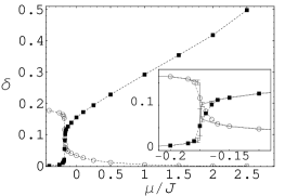
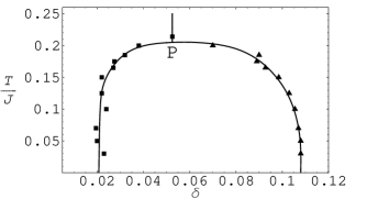
(a)	(b)

Figure 14: (a) Hole concentration $\delta=\rho/2=\frac{1}{2}\langle t_{h}^{\dagger}t_{h}\rangle$ (filled squares) and magnon density $\sum_{\alpha}\frac{1}{2}\langle t_{\alpha}^{\dagger}t_{\alpha}\rangle$ (circles) as a function of the chemical potential $\mu$ at $T/J=0.03$. The small inlay shows a detailed view to the $\mu$ region in which the hole-pair density jumps to a finite value. (b) Hole densities of the coexisting phases on the first order transition line from (almost) zero to finite hole density at $\mu\!=\!\mu_{c}$ as a function of temperature.

After numerically solving the projected $SO(5)$ model, we obtain Fig. 14a, which gives the mean hole-pair and magnon densities as a function of the chemical potential for $T/J\!=\!0.03$ and their $T\!\to\!0$ extrapolations Jöstingmeier et al. (2003). Similar to the mean-field results, a jump in the densities can be clearly seen at $\mu_{c}\!=\!-0.175$, with a shift in respect to the mean-field value due to the stronger fluctuations of hole pairs, as seen in the Gaussian contributions Zhang et al. (1999). The nature of the phase transition at $\mu\!=\!\mu_{c}$ can be determined by studying histograms of the hole-pair distribution for fixed $\mu\!=\!\mu_{c}$. While in a homogeneous phase the density peaks at its mean value, at $\mu\!=\!\mu_{c}$ we obtain two peaks, which indicates a first-order transition with a phase separation between (almost) hole-free regions and regions with high hole-pair density. From Fig. 14b we see that the transition is of first order for $T\!<\!T_{P}\!=\!(0.20\pm 0.01)J$ at $\mu\!=\!\mu_{P}\!=\!(-0.168\pm 0.002)J$. Above $T_{P}$, the histograms show strongly fluctuating hole-pair densities, suggesting the presence of critical behavior.

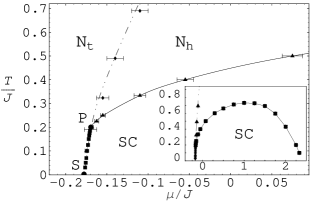
(a)	(b)

Figure 15: (a) Phase diagram of the projected $SO(5)$ model (see Eq. (69) with $J_{c}=J_{S}$) in D=2: The squares between S and the tricritical point P trace the first-order line of phase separation. The solid line from P to the right edge of the plot traces the Kosterlitz-Thouless transition between the SC and the normal state. The dashed line separating $N_{t}$ (=triplet dominated region) and $N_{h}$ (=hole pair dominated region) describes the line of equal AF and SC correlation lengths. The small inlay shows the same phase diagram on a larger $\mu$ scale, covering the whole KT phase. The tricritical point P appears as a result of the Mermin-Wagner theorem, which does not allow spin ordering in D=2 at finite temperature. (b) Energy of a single magnon excitations in the projected $SO(5)$ model as a function of the chemical potential. This corresponds to the resonance energy of the $(\pi,\pi)$ peak of the spin correlations in the fermionic model (magnons are defined to carry the momentum of the AF order). The numbers in parentheses indicate the peak weights, i.e. the area under the peak. ($20\!\times\!20$ lattice at temperature $T/J\!=\!0.1$). (from Ref. Jöstingmeier et al. (2003))

Based on these results, the phase diagram of the 2D projected $SO(5)$ model is obtained in Fig. 15. Unlike the generic three dimensional phase diagrams presented in Fig. 10, there can be no finite temperature Neel transition in D=2 because of the Mermin-Wagner theorem. On the other hand, a continuous transition of the Kosterlitz-Thouless (KT) type is possible for the SC to normal state transition at finite temperature. The 3D phase diagram shown in Fig. 10a takes the form of Fig. 15 in D=2, where the first order line separating the AF and SC phases merges into the continuous KT transition at a tricritical point P. The SC phase with finite superfluid density $\rho_{s}$ is identified by a power-law decay of the SC correlation function:

$$C_{h}{(r)}=\big{(}t_{h}^{\dagger}{(r)}+t_{h}{(r)}\big{)}\big{(}t_{h}^{\dagger}{(0)}+t_{h}{(0)}\big{)}\;.$$

The KT transition line in Fig. 15a separates power-law ($C_{h}{(r)}\propto r^{-\alpha}$) from rapid exponential decay ($C_{h}{(r)}\propto\mbox{e}^{-\lambda r}$). A reliable and accurate distinction between these two decay behaviors requires a finite-size scaling with large system sizes, as well as an efficient QMC estimator for the Green functions appearing in the correlation function. With its non-local update scheme and with our new estimators for arbitrary Green functions, SSE provides both (for details see Ref. Dorneich and Troyer (2001)). An alternative method for detecting a KT transition exploits the fact that the superfluid density jumps from zero to a finite value at the KT temperature $T_{KT}$Nelson and Kosterlitz (1977). Within SSE the superfluid density can be measured quite easily by counting winding numbersHarada and Kawashima (1997). Numerically, this criterion is preferable to the arduous process of direct determination of decay coefficients. Fig. 15a plots the phase diagram obtained by applying both criteria independently. The figure shows that the projected $SO(5)$ model indeed has a KT phase with quasi long-range order whose dome-like form in $\mu$-$T$ space looks like that of the HTSC cuprates. Both criteria produce the same clearly pronounced phase separation line. It is well known that a similar transition cannot occur for antiferromagnetsChakravarty et al. (1988) and that the finite-$T$ AF correlation length $\xi$ is always finite and behaves like $\xi\propto\mbox{e}^{2\pi\rho_{s}/k_{B}T}$, with $\rho_{s}$ being the spin stiffness. This fact is confirmed by our numerical results.

One condition required for an $SO(5)$ symmetric point is that the formation energies of hole-pair bosons and of magnons are identical. This condition is fulfilled along the line from $S$ to the tricritical point $P$ in Fig. 15. Another necessary condition is that hole pairs and magnons behave in the same way at long distances. This condition is fulfilled on the dashed line in Fig. 15, where the AF and SC correlation lengths $\xi$ become equal. Interestingly, these two conditions are met (within error bar accuracy) at the tricritical point P. Of course, the correlation length is still finite here; however, we find relatively large $\xi$ values of order 10 to 15 in the immediate vicinity of point P, demonstrating the importance of $SO(5)$ critical fluctuations in this region.

In addition, in realistic electron systems, the long-range part of the Coulomb repulsion between the doubly-charged hole pairs disfavors phase separation, while extended short ranged interactions described by Eq. (84) could lead to the formation of stripes and checkerboard types of states, as discussed in section IV.2. To study the effect of off-site Coulomb interaction, we have added additional nearest-neighbor and next-nearest-neighbor Coulomb repulsions $V_{c}$ and $V_{c}^{\prime}\!=\!0.67\!\;V_{c}$ to the projected $SO(5)$ model. Indeed, a relatively modest Coulomb repulsion of $V_{c}/J\!\approx\!0.2$ is enough to completely destroy the phase separation. Thus, one interesting effect of Coulomb interaction in two dimensions is to push down the tricritical point into a quantum-critical point at $T\!=\!0$. In section IV.1 and in Fig. 9c, we showed that the $SO(5)$ symmetric behavior is recovered at the special point when a direct first order transition changes into two second order transitions. Therefore, the extended Coulomb interaction plays the role of the $w$ parameter in Fig. 9c and could restore the $SO(5)$ symmetry at the quantum critical point.

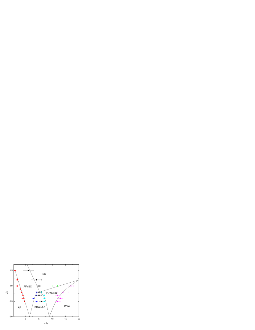
Figure 16: The phase diagram of the extended $SO(5)$ model obtained by the QMC simulation. The parameters used in simulation are $\Delta_{s}=4.8$, $V_{c}=4.1010$, $V_{c}^{\prime}=3.6329$ and $J_{\pi}=V_{\pi}=0$. The lines are guides to the eye only. The overall topology of the phase diagram agrees well with the global phase diagram presented in Fig. 13.

When larger values of extended interaction parameters in Eq. (84) are considered, new insulating phases are expected, following from the general discussions in section IV.2 and Fig. 13. Indeed, Chen et al Chen et al. (2003a) have performed extensive QMC simulation of the $SO(5)$ model and have determined its generic phase diagram, as shown in Fig. 16. In addition to the AF and SC phases, there is an insulating pair-density-wave state around doping range of $x=1/8$, where hole pairs form a checkerboard state in the AF ordered background, as depicted in Fig. 12d. Near the phase boundaries between the AF, PDW and SC phases, there are mixed phases with coexisting order. The topology of the phase diagram obtained from the QMC simulation agrees well with the mean field theory of the extended $SO(5)$ model. One of the main features of the $SO(5)$ theory is that it provides an elegant explanation for the neutron resonance peak observed in some HTSC cuprates at $q\!=\!(\pi,\pi)$Demler and Zhang (1995); Zhang (1997). We refer the reader to the detailed discussion of the resonance mode in section VI. Experiments show that the resonance energy $\omega_{\mbox{\scriptsize res}}$ is an increasing function of $T_{c}$, i.e. $\omega_{\mbox{\scriptsize res}}$ increases as a function of doping in the underdoped region and decreases in the overdoped regionFong et al. (2000). Fig. 15b plots the resonance frequency determined from the spin correlation spectrum obtained for the projected $SO(5)$ model. As illustrated in Fig. 8, the spin-wave excitations are massless Goldstone modes in the AF phase at $\mu\!<\!\mu_{c}$ (and $T\!=\!0$) and become massive when entering into the SC phase. $\omega_{\mbox{\scriptsize res}}$ increases monotonically up to the optimal doping $\mu_{\mbox{\scriptsize opt}}\!\approx\!1$. In the overdoped range of the simple $SO(5)$ model, however, $\omega_{\mbox{\scriptsize res}}$ is increasing more, in contrast to what happens in the cuprates. The resonance peak continuously loses weight as $\mu$ increases, which is consistent with experimental observations Fong et al. (2000).

A comparison of the critical temperature $T_{c}$ obtained from Fig. 15 and the resonance frequency $\omega_{\mbox{\scriptsize res}}$ at optimal doping yields the ratio $T_{c}/\omega_{\mbox{\scriptsize res,opt}}\!=\!0.23$. Again, this is in qualitative accordance with the corresponding ratio for $\mathrm{YBa_{2}Cu_{3}O_{6+x}}$, for which the experimentally determined values $T_{c}\!=\!93\,\mbox{K}$ (thus $k_{B}T_{C}\!=\!8.02$ meV) and $\omega_{\mbox{\scriptsize res,opt}}\!=\!41$ meV yield $T_{c}/\omega_{\mbox{\scriptsize res,opt}}\!=\!0.20$.

Now we turn to the numerical simulations of the $SO(5)$ models in D=3. Two aims motivate our studies of the projected $SO(5)$ model in three dimensions (3D). First, we expect to find an AF and SC phase with real long-range order. We need to determine which of the two types of phase diagrams introduced in section IV.1 (see Fig. 10) is realized in the numerical simulations. Second, we would like to determine whether the projected $SO(5)$ model has a certain multi-critical point at which the $SO(5)$ symmetry is asymptotically restored. Since the cuprates have a pronounced 2D layer structure with relatively weak couplings between adjacent CuO₂ planes, the 2D and the isotropic 3D model (discussed here) should be two extreme poles for the possible range of properties of real HTSC materials. Most numerical data reviewed here have been obtained by a finite-size scaling with lattice sites up to 10,000. Dorneich and Troyer (2001); Jöstingmeier et al. (2003); Dorneich et al. (2002b, a)

The phase diagram and the scaling behavior of the classical $SO(5)$ model has been studied in detail by Hu in Ref. Hu (2001) by means of classical Monte Carlo simulations (MC). Classical MC are by orders of magnitude easier to perform and less resource demanding than QMC simulations; hence, very large system sizes can be simulated and highly accurate data can be obtained. The classical $SO(5)$ model can be obtained directly from the quantum $SO(5)$ model by taking the expectation value of the Hamiltonian in the variational state, as given by Eq. (83) and assuming a constant value of $\theta(x)$. It takes the form:

$$H=-J\sum_{\langle x,x^{\prime}\rangle}m_{a}(x)m_{a}(x^{\prime})+g\sum_{x}m^{2}_{\alpha}(x)+w\sum_{x}m^{2}_{\alpha}(x)m^{2}_{i}(x),$$ (85)

where $g=\Delta_{s}-\tilde{\Delta}_{c}$ is the quadratic symmetry breaking term, and $w$ is an additional quartic symmetry breaking term. Hu established the $T(g)$ phase diagram, which is of the type illustrated in Fig. 10a. The model has an AF and SC phase which meet at a bicritical point $(T_{bc},g_{bc}\!=\!0)$. The boundary lines between the disordered and AF phases, and between the disordered and SC phases merge tangentially at the bicritical point, which is an important characteristics of $SO(5)$ symmetry Hu (2001). The following scaling properties were determined by Hu and will be used to study the restoration of $SO(5)$ symmetry in the projected $SO(5)$ model.

For an analysis of the crossover phenomenon, an Ansatz for the behavior of the helicity modulus $\Upsilon$ in the range $T\!<\!T_{c}(g)$ and $g\!>\!0$ is used, which is suggested by scaling theoryHu (2001):

$$\Upsilon(T,g)\propto(g-g_{bc})^{\nu_{5}/\phi}\times f\big{(}(T/T_{bc}-1)\big{/}(g-g_{bc})^{1/\phi}\big{)}\,.$$ (86)

Here, $\nu_{5}$ is the critical exponent for correlation length at $n\!=\!5$ and $\phi$ the crossover exponent. Using (86), the values of $\nu_{5}$ and $\phi$ can be determined in two steps. First, performing a $g$ scan of $\Upsilon(T\!=\!T_{bc},g)$ returns the ratio $\nu_{5}/\phi$:

$$\Upsilon(T_{bc},g)/\Upsilon(T_{bc},g^{\prime})=\big{(}(g-g_{bc})/(g^{\prime}-g_{bc})\big{)}^{\nu_{5}/\phi}\,.$$ (87)

Then, $\phi$ is obtained from the slopes $\frac{\partial}{\partial T}(\Upsilon\big{(}T,g)/\Upsilon(T,g^{\prime})\big{)}$ via

$$\phi=\ln\Big{(}\frac{g_{2}-g_{bc}}{g_{1}-g_{bc}}\Big{)}\bigg{/}\ln\bigg{(}\frac{\partial}{\partial T}\frac{\Upsilon(T,g_{1})}{\Upsilon(T,g_{1}^{\prime})}\Big{|}_{T=T_{bc}}\Big{/}\frac{\partial}{\partial T}\frac{\Upsilon(T,g_{2})}{\Upsilon(T,g_{2}^{\prime})}\Big{|}_{T=T_{bc}}\bigg{)}\,$$ (88)

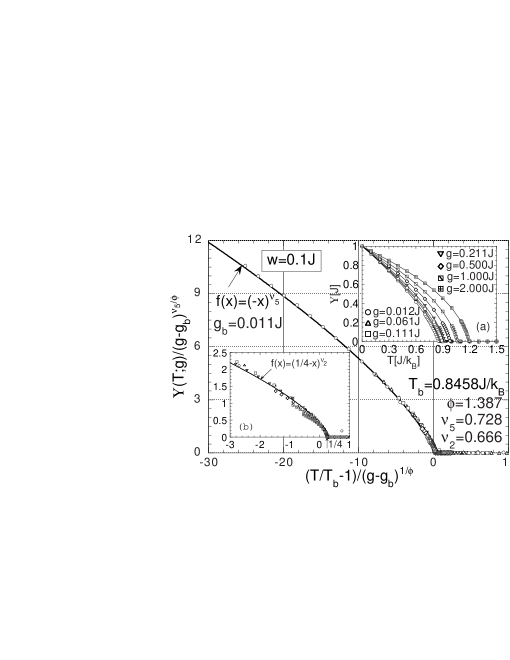
Figure 17: Scaling of the superfluid density near the $SO(5)$ bi-critical point obtained by the classical Monte Carlo simulations. The critical behavior of the superfluid density for various $g$ fit into a single scaling curve, from which $SO(5)$ scaling exponents were obtained. Reproduced from Ref. Hu (2001).

if $g_{1}$, $g_{1}^{\prime}$, $g_{2}$, and $g_{2}^{\prime}$ are related by $(g_{1}-g_{bc})/(g_{1}^{\prime}-g_{bc})\!=\!(g_{2}-g_{bc})/(g_{2}^{\prime}-g_{bc})>0$. From the scaling plots presented in Fig.17, Hu finds the values $\nu_{5}/\phi\!=\!0.523\pm 0.002$ and $\phi\!=\!1.387\pm 0.030$.

According to the scaling Ansatz in (86), the transition lines between the disordered and AF phases, and between the disordered and SC phases near the bicritical point should be of the form

$$B_{2}\cdot(g-g_{bc})^{1/\phi}=\frac{T_{c}(g)}{T_{bc}}-1\quad\;\mbox{and}\quad\;B_{3}\cdot(g_{bc}-g)^{1/\phi}=\frac{T_{N}(g)}{T_{bc}}-1\,.$$ (89)

The ratio $B_{2}/B_{3}$ should be given by the inverse ratio between the AF and SC degrees of freedom, i.e.

$$B_{2}/B_{3}\!=\!3/2\,.$$ (90)

The values numerically determined by Hu indeed have the correct ratio: $B_{2}\!=\!1/4$ and $B_{3}\!=\!1/6$.

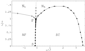
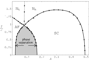
(a)	(b)

Figure 18: (a) The $T(\mu)$ phase diagram of the three-dimensional projected $SO(5)$ model with $J_{s}\!=\!J_{c}/2$ and $\Delta_{s}\!=\!\Delta_{c}\!=\!J$. N_h is the hole-pair dominated part, N_t the triplet dominated part of the high-temperature phase without long-range order. The separation line between N_h and N_t is the line of equal spatial correlation decay of hole-pairs and bosons. (b) The $T(\delta)$ phase diagram of the 3D projected $SO(5)$ model as a function of hole doping $\delta=n_{h}/2$. The first order transition line from $S$ to $P$ in the $T(\mu)$ diagram becomes a “forbidden region” due to phase separation. These two phase diagrams are consistent with those presented in Fig. 10a-b based on general arguments.

We now proceed to the phase diagram of the 3D quantum $SO(5)$ model Dorneich et al. (2002b, a). Figure 18 shows the AF and SC phases, as expected. Furthermore, the two phase transition lines merge tangentially into a multi-critical point (at $T_{bc}\!=0.960\pm 0.005$ and $g_{bc}\!=\!-0.098\pm 0.001$) just as in the classical $SO(5)$ system Hu (2001). The line of equal correlation decay of hole-pairs and triplet bosons also merges into this bicritical point $P$ – a necessary condition at this point for the restoration of $SO(5)$ symmetry. Unlike the corresponding phase in the classical model Hu (2001), the SC phase only extends over a finite $g$ range due to the hardcore constraint of the hole-pair bosons and agrees with experimentally determined phase diagrams of the cuprates. Obviously, the quantum mechanical $SO(5)$ model is ‘more physical’ in this aspect than the classical $SO(5)$ model. In real cuprates the ratio between the maximum temperatures $T_{c}$ and $T_{N}$ is about 0.17 to 0.25, whereas in the projected $SO(5)$ model we obtain the values $T_{c}/J\!=\!1.465\pm 0.008$ at $\mu_{\mathit{opt}}/J\!\approx\!1.7$ and $T_{N}/J\!=1.29\pm 0.01$ at $\mu\to\-\infty$; hence, $T_{c}$ is slightly larger than $T_{N}$. In order to obtain realistic values for the transition temperatures, it is necessary to include the $J_{\pi}$ and $V_{\pi}$ terms in Eq. (84). These terms represent the repulsion between the magnons and the hole pairs. If we take the expectation values of the hole pair operators, these terms effectively represent a doping dependent $J_{s}$, which can produce a more realistic phase diagram. Such terms break the $SO(5)$ symmetry of the static potential at T=0 (see Section III.3 after equation (67)). However, the static symmetry may still be recovered at the bicritical point, as discussed in Section IV.1. At this point we are primarily concerned with the multi-critical behavior, so we stay with the simple $SO(5)$ model.

A closer look at the phase transition line between the points $S$ and $P$ (see Fig. 18) reveals that this line is slightly inclined, unlike the vertical line seen in the classical $SO(5)$ model. This indicates that a finite latent heat is connected with the AF-SC phase transition. In addition, this means that $\mu$ is not a scaling variable for the bicritical point $P$, as it is in the classical model. The result in Fig.18 shows a phase separation regime at $\mu=\mu_{c}$ on the entire transition line from S to P.

We now review the results of a scaling analysis for the 3D quantum $SO(5)$ model, similar to the one performed by Hu Hu (2001) in a classical $SO(5)$ system Dorneich et al. (2002a). From this analysis we also find that the $SO(5)$ symmetry is restored in the region around the bicritical point ($T_{bc}\!=\!0.96$, $\mu\!=\!-0.098$).

We have determined the critical exponents for the onset of AF and SC orders for various chemical potentials as a function of temperature. Far into the SC range, at $\mu\!=\!1.5$, we find that the SC helicity modulus follows the scaling form Fisher et al. (1973)

$$\Upsilon\propto(1-T/T_{c})^{\nu}\quad\;\mbox{with}\quad\;\nu=0.66\pm 0.02\,,$$

which agrees with the values obtained by both the $\epsilon$-expansion and numerical analysis of a 3D XY model. On the AF side, error bars are larger. For $\mu=-2.25$,

$${C_{AF}(\infty)}\propto(1-T/T_{c})^{\beta_{3}}\quad\;\mbox{with}\quad\;\beta_{3}=0.35\pm 0.03,$$

as expected for a 3D classical Heisenberg model.

To determine $\nu$ and $\phi$, we use Eqs. (87) and (88), which express the scaling behavior in the crossover regime (cf. Ref. Hu (2001)). We obtain the ratio

$$\nu_{5}/\phi=0.52\pm 0.01,$$

which matches the results of the $\epsilon$-expansionKosterlitz et al. (1976); Hu and Zhang (2000). $\phi$ is then obtained by using (88). The result is

$$\phi=1.43\pm 0.05\,$$

which also agrees with the $\epsilon$-expansion for an $SO(5)$ bicritical point and with the results of Ref. Hu (2001).

Let us finally return to the comment by Aharony Aharony (2002), who, via a rigorous argument, demonstrated that the decoupled fixed point is stable, as opposed to the biconical and $SO(5)$ fixed points. However, he also commented that the unstable flow is extremely slow for the $SO(5)$ case due to the small crossover exponent.

The scaling analysis of the 3D projected $SO(5)$ model has produced a crossover exponent which matches the value obtained from a classical $SO(5)$ model and from the $\epsilon$-expansion. This provides strong evidence that the static correlation functions at the $SO(5)$ multicritical point are controlled by a fully $SO(5)$ symmetric point, at least in a large transient region. However, the isotropic $SO(5)$ and biconical fixed points have very similar critical exponents. Thus, given the statistical and finite-size errors, as well as the errors due to the extrapolation of the $\epsilon$-expansion value to $\epsilon=1$, we cannot exclude the possibility that the multicritical point on the phase diagram is actually the biconical one. On the other hand, the biconical fixed point should be accompanied by a uniform AF/SC mixed region (as a function of chemical potential), which was not observed. The decoupled fixed point appears to be the least compatible with the numerical results presented above. Even if the bicritical point is fundamentally unstable, as suggested by Aharony in Aharony (2002), one would have to come unrealistically close to $T_{bc}$ to observe this. For example, for the projected $SO(5)$ models Ref. Arrigoni and Hanke (1999) estimated that deviations from the $SO(5)$ behavior may be observed only when the reduced temperature becomes smaller than $|T-T_{bc}|/T_{bc}<10^{-11}$. On the other hand, the other scaling variables, although initially of the order of $1$, rapidly scale to zero due to the large, negative exponents. Therefore, the $SO(5)$ regime starts to become important as soon as the AF and SC correlation lengths become large and basically continues to affect the scaling behavior of the system in the whole accessible region.

Summarizing, the accurate QMC calculations show that the projected $SO(5)$ model which combines the idea of $SO(5)$ symmetry with a realistic treatment of the Hubbard gap, is characterized by an $SO(5)$ symmetric bicritical point, at least within a large transient region. Possible flow away from this symmetric fix point occurs only within a narrow region in reduced temperature, making it impossible to observe either experimentally or numerically. This situation is common to many systems in condensed matter physics. For example, due to the well-known Kohn-Luttinger effect Kohn and Luttinger (1965), the Fermi-liquid fixed point is always unstable towards a SC state. However, this effect is experimentally irrelevant for most metals since it only works at extremely low temperatures. Another example is the “ordinary” superconductor to normal-state transition at $T_{c}$. Strictly speaking, due to the coupling to the electromagnetic field this fixed point is always unstable Halperin et al. (1974). However, this effect is experimentally irrelevant since the associated critical region is extremely small. Similarly, irrespective of the question of ultimate stability, the $SO(5)$ fixed point is a robust one in a large transient regime, and it can control the physics near the AF and SC transitions. For all practical purposes, the multi-critical point is dominated by the initial flow toward the $SO(5)$ symmetric behavior.

V MICROSCOPIC ORIGIN OF THE SO(5) SYMMETRY

V.1 Quantum lattice models with exact SO(5) symmetry

Soon after the general $SO(5)$ theory was proposed, a class of microscopic fermion models with exact $SO(5)$ symmetry was constructedRabello et al. (1998); Henley (1998); Burgess et al. (1998); Scalapino et al. (1998); Wu et al. (2003a). These models fall into three general classes. The first class contains models with two sites per unit cell, such as the ladder and the bi-layer models. In these models, a simple condition among the local interaction parameters ensures the full quantum $SO(5)$ symmetry. The second class contains models with only one site in the unit cell but with longer ranged interactions. The third class contains higher spin fermion models, in particular the spin $3/2$ Hubbard model. Remarkably, in this case the models are always $SO(5)$ symmetric without any fine tuning of the local interaction parameters and doping level.

The microscopic $SO(5)$ symmetric models in the ladder or bi-layer models were first constructed by Scalapino, Zhang and Hanke (SZH)Scalapino et al. (1998) and have been studied extensively both analytically and numerically Lin et al. (1998); Arrigoni and Hanke (1999); Furusaki and Zhang (1999); Schulz (1998); Shelton and Senechal (1998); Bouwknegt and Schoutens (1999); Duffy et al. (1998); Eder et al. (1999); Frahm and Stahlsmeier (2001); Hong and Salk (1999). In these models, there are two sites and $4^{2}=16$ states in the unit cell. In section III.1, we already discussed the construction of $SO(5)$ symmetry operators in terms of the fermion operators for two sites in the unit cell. Here we shall address the question of whether the microscopic Hamiltonian commutes with the $SO(5)$ symmetry generators. Three interaction parameters, $U$, $V$ and $J$, fully characterize the most general local interactions on the two sites, which takes the form

$$H(x)=U(n_{c\uparrow}-\frac{1}{2})(n_{c\downarrow}-\frac{1}{2})+(c\rightarrow d)+V(n_{c}-1)(n_{d}-1)+J\vec{S}_{c}\vec{S}_{d}-\mu(n_{c}+n_{d}).$$ (91)

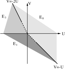
(a)	(b)

Figure 20: (a) Under the condition specified by Eq. (92), the 16 states on a rung are classified into 6 groups, each transforming irreducibly under the $SO(5)$ group. $|\Omega\rangle$ is an $SO(5)$ singlet state; $n_{a}|\Omega\rangle$ desribes five states that transform as $SO(5)$ vectors; $\Psi_{\alpha}^{\dagger}|\Omega\rangle$ are four states that form an $SO(5)$ spinor; four states $\Psi_{\alpha}|\Omega\rangle$ also correspond to a spinor; $R_{\alpha\beta}\Psi_{\alpha}\Psi_{\beta}|\Omega\rangle$ and $R_{\alpha\beta}\Psi^{\dagger}_{\alpha}\Psi^{\dagger}_{\beta}|\Omega\rangle$ are two $SO(5)$ singlet states. The figure also gives energies of all multiplets for the $SO(5)$ symmetric ladder model described by equations (91) and (92). (b) Strong coupling phase diagram of the $SO(5)$ symmetric ladder model in the $(U,V)$ space. The $E_{0}$, $E_{1}$ and $E_{3}$ phases are regions in parameter space where the respective states have the lowest energy.

This Hamiltonian can be solved easily for the $16$ states on two sites and the 6 energy levels are given in Fig. 20. Since the $SO(5)$ symmetry generators can be expressed in terms of the microscopic fermion operators, we can easily determine the transformation properties of these states under the $SO(5)$ group. There are three $SO(5)$ singlet states, and two fermionic quartet states, which form the fundamental spinor representations of $SO(5)$. We see that the four fermionic states in each group are always degenerate, without any fine tuning of the interaction parameters. The three spin triplet states at half filling and the two paired states away from half-filling form the five dimensional vector representation, but they are only degenerate if we specify one condition, namely

$$J=4(U+V).$$ (92)

This condition ensures the local $SO(5)$ symmetry within the unit cell. Remarkably, under this condition, a global $SO(5)$ symmetry is also obtained for a bi-partite lattice including nearest-neighbor hopping. This is best demonstrated when we write the model in a manifestly $SO(5)$ covariant manner. On a bi-partite lattice, we introduce the four-component spinor operator

$$\Psi_{\alpha}(x\in even)=\left(\begin{array}[]{c}c_{\sigma}(x)\\ d^{\dagger}_{\sigma}(x)\end{array}\right)\ \ \ \Psi_{\alpha}(x\in odd)=\left(\begin{array}[]{c}d_{\sigma}(x)\\ c^{\dagger}_{\sigma}(x)\end{array}\right).$$ (97)

The microscopic Hamiltonian including intra-rung hopping $t_{\bot}$ and inter-rung hopping $t_{\parallel}$ is given by

$$H=-2t_{\parallel}\sum_{\langle x,x^{\prime}\rangle}(c^{\dagger}_{\sigma}(x)c_{\sigma}(x^{\prime})+d^{\dagger}_{\sigma}(x)d_{\sigma}(x^{\prime}))-2t_{\bot}\sum_{x}(c^{\dagger}_{\sigma}(x)d_{\sigma}(x)+h.c)+\sum_{x}H(x).$$ (98)

Under condition (92), this Hamiltonian can be expressed in a manifestly $SO(5)$ invariant manner:

$$H=2t_{\parallel}\sum_{\langle x,x^{\prime}\rangle}(\Psi_{\alpha}(x)R^{\alpha\beta}\Psi_{\beta}(x^{\prime})+h.c.)+t_{\bot}(\Psi_{\alpha}R^{\alpha\beta}\Psi_{\beta}+h.c.)+\sum_{x}\frac{J}{4}L_{ab}^{2}(x)+(\frac{J}{8}+\frac{U}{2})(\Psi^{\dagger}_{\alpha}\Psi_{\alpha}-2)^{2},$$ (99)

where the $R$ matrix is defined in the Appendix. This model was originally constructed for the two-legged ladder system, but it works equally well for a two dimensional bi-layer system.

The phase diagram of this $SO(5)$ symmetric model has been studied extensively in the literature. This simple model has a rich and rather complex phase diagram, depending on the coupling strength and doping. However, because of the constraints imposed by the $SO(5)$ symmetry, the phase diagram is much better understood compared to other related models. In the strong coupling limit, three phase boundary lines are determined from the level crossing of the bosonic states on two sites. At $V=-2U$, the $E_{0}$ state becomes degenerate with the $E_{3}$ states; at $V=-U$, the $E_{0}$ state becomes degenerate with the $E_{1}$ states; finally, at $V=0$ the $E_{1}$ states become degenerate with the $E_{3}$ states. The strong coupling phase diagram at half-filling is shown in Fig. 20b.

In the strong coupling $E_{0}$ phase, a robust ground state is obtained as a product of $SO(5)$ singlets on the rungs. This type of insulating state does not break any lattice translational or internal rotational symmetry. Since there are two electrons per unit cell, this insulating state is also adiabatically connected to the band insulator state. This state is separated from the excited $SO(5)$ quintet vector states by a finite energy gap, $\Delta=E_{1}-E_{0}=J$. In this regime, we consider the low energy manifold consisting of six states, namely one $E_{0}$ state $|\Omega\rangle$ and five $E_{1}$ states $n_{a}|\Omega\rangle$ per rung. The low energy effective Hamiltonian can be obtained easily by the second order strong coupling expansion and is exactly given by the $SO(5)$ quantum non-linear $\sigma$ model Hamiltonian given in Eq. (53), with $\chi^{-1}=J$ and $\rho=J_{\parallel}=t^{2}_{\parallel}/(U+J/2)$. The operators $L_{ab}$ and $n_{a}$ act on the six states in the following way:

$$L_{ab}(x)|\Omega(x)\rangle=0\ \ ,\ \ L_{ab}(x)|n_{c}(x)\rangle=i\delta_{bc}|n_{a}(x)\rangle-i\delta_{ac}|n_{b}(x)\rangle$$

$$n_{a}(x)|\Omega(x)\rangle=|n_{a}(x)\rangle\ \ ,\ \ n_{a}(x)|n_{b}(x)\rangle=\delta_{ab}|\Omega(x)\rangle.$$ (100)

Since the quantum model is exactly $SO(5)$ symmetric, the anisotropy term $V(n)$ vanishes identically. Therefore, we see that the $SO(5)$ quantum non-linear $\sigma$ model, phenomenologically introduced in section III.2, can indeed be rigorously derived from the microscopic SZH model defined on a ladder and on a bi-layer.

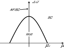
Figure 21: Phase diagram of the bi-layer $SO(5)$ model plotted as $J_{\parallel}/J$ versus $\mu$. The entire phase transition line from the Mott phase into any of the ordered phases is a second order quantum phase transition. The Mott insulating state has 5 massive collective modes. The $SO(5)$ symmetric AF/SC uniform mixed state at half-filling has 4 gapless collective modes. The SC state has a spin triplet $\pi$ resonance mode and one massless charge Goldstone mode.

In the $E_{0}$ regime, the SZH model on the half-filled ladder has a $SO(5)$ rung singlet ground state with a finite gap towards the $SO(5)$ quintet excitations. A chemical potential term of the order of the gap induces a second order quantum phase transition into the SC phase. On the other hand, the SZH model on the bi-layer has a quantum phase transition even at half-filling, when $J_{\parallel}/J\sim 1$. For $J>J_{\parallel}$, the ground state is a Mott insulator without any symmetry breaking with a finite gap towards the quintet excitations. For $J<J_{\parallel}$, the ground state is classically ordered and breaks the $SO(5)$ symmetry spontaneously by aligning the superspin in a particular direction, which can be either AF or SC. Since the residual symmetry is $SO(4)$, the Goldstone manifold of the $\sigma$ model is the four dimensional sphere $SO(5)/SO(4)=S^{4}$. Away from half-filling, the $SO(5)$ symmetry is broken by the chemical potential term. According to Table I, the $\pi$ operators carry charge $\pm 2$, and we have $[H,\pi^{\dagger}_{\alpha}]=2\mu\pi^{\dagger}_{\alpha}$. However, although the Hamiltonian does not commute with all the $SO(5)$ generators, it still commutes with the Casimir operator $L_{ab}^{2}$. For this reason, all states are still classified by $SO(5)$ quantum numbers and the $SO(5)$ symmetry makes powerful predictions despite a broken symmetry away from half-filling. The phase diagram for the two dimensional SZH bi-layer model is shown in Fig. 21. For $J_{\parallel}\gg J$, the ground state is classically ordered. The chemical potential induces a quantum phase transition from the $SO(5)$ uniform mixed AF/SC state to the SC state at $\mu=0$. This transition is exactly the superspin flop transition discussed in section III.2. For $J_{\parallel}\ll J$, the ground state is quantum disordered at half-filling. A second order quantum phase transition from the singlet Mott insulator state to the SC state is induced at finite $\mu=\mu_{c}$. The exact $SO(5)$ bi-layer model offers an ideal theoretical laboratory to study the collective modes, especially the $\pi$ resonance mode discussed in section VI, since their sharpness is protected by the exact $SO(5)$ symmetry. The Mott phase has five massive collective modes, a doublet of charge modes and a triplet of spin modes. The energy of the two charge modes splits at finite chemical potential, and the energy of one of the charge modes vanishes at the second order phase transition boundary. This charge mode continues into the SC phase as the phase Goldstone mode. The spin triplet mode of the Mott phase continues smoothly into the SC phase and becomes the pseudo-Goldstone mode, or the $\pi$ resonance mode of the SC phase. The ordered phase at half-filling has four Goldstone modes. The direction of the order parameter can be smoothly rotated from AF to SC at half-filling. When the order parameter points in the AF direction, the four Goldstone modes decompose into two spin wave modes and two charge modes. When the order parameter is rotated into the SC direction, the four Goldstone modes decompose into a spin triplet and a Goldstone phase mode. The energy of the triplet Goldstone mode (the massive $\pi$ mode) increases continuously with the chemical potential, while the phase Goldstone mode remains gapless.

Having discussed the $E_{0}$ regime at length, let us now turn to the $E_{1}$ regime, where the $SO(5)$ quintet state has the lowest energy. In this case, we can restrict ourselves to the low energy manifold of five states on each rung. The effective theory within this low energy manifold can again be obtained by the strong coupling second order perturbation theory, and is given by

$$H=K\sum_{\langle x,x^{\prime}\rangle}L_{ab}(x)L_{ab}(x^{\prime}),$$ (101)

where $K=t^{2}_{\parallel}/(U/2-J/4)$. This effective Hamiltonian is the $SO(5)$ generalization of the AF spin 1 Heisenberg model. Here we must distinguish between the one dimensional ladder model and the two dimensional bi-layer model. In one dimensional models, the ground state is separated from the $SO(5)$ vector excitation by a finite energy gap. In fact, an exact ground state can be constructed for the $SO(5)$ vector model by generalizing the AKLT model for the spin 1 chain. Such a state also preserves the lattice translational and internal rotational symmetry. However, in two dimensional bi-layer models, the effective exchange coupling between the $SO(5)$ vectors will lead to a state with spontaneously broken $SO(5)$ symmetry, with the $SO(5)$ adjoint order parameter $\langle L_{ab}\rangle\neq 0$. This order parameter is formed by the linear superposition of two $SO(5)$ vector states, $n_{a}$ and $n_{b}$. Without loss of generality, let us consider the case where $\langle L_{15}\rangle\neq 0$. In this case, the $SO(5)$ generators $L_{15}$, $\{L_{23},L_{24},L_{34}\}$ leaves the state invariant. These set of generators form a $U(1)\times SU(2)$ symmetry group. Therefore, the Goldstone manifold is the coset space

$$SO(5)/\left(U(1)\times SU(2)\right)=CP_{3},$$ (102)

where $CP_{3}$ is the six (real) dimensional complex projective space, which can be described by the complex coordinates $(z_{1},z_{2},z_{3},z_{4})$, satisfying $|z_{1}|^{2}+|z_{2}|^{2}+|z_{3}|^{2}+|z_{4}|^{2}=1$ and with the points related by a $U(1)$ gauge transformation $z_{i}\rightarrow e^{i\alpha}z_{i}$ identified. Since the $CP_{3}$ manifold is six dimensional, there are six Goldstone bosons in this case. Here we see that there is an important difference between the $SO(5)$ symmetric SZH model and the $SO(3)$ symmetric Heisenberg model. In the Heisenberg model, the vector representation is identical the adjoint representation, there is only one type of classically ordered AF state. In the $SO(5)$ case, the symmetry breaking can occur either in the vector or the adjoint representations of the $SO(5)$ group, which are inequivalent, and the resulting Goldstone manifolds are $S^{4}$ and $CP_{3}$, respectively. The adjoint symmetry breaking pattern has been used by Murakami, Nagaosa and Sigrist to unify $p$ wave SC with ferromagnetismMurakami et al. (1999).

In the weak coupling limit, powerful renormalization group (RG) analysis has been applied to study the $SO(5)$ symmetry in ladder models. The main conclusions are similar to the strong coupling analysis; therefore, we will only review the most remarkable and distinct results. Lin, Balents and FisherLin et al. (1998), Arrigoni and HankeArrigoni and Hanke (1999), SchulzSchulz (1998), Shelton and SenechalShelton and Senechal (1998) carried out detailed RG analysis and showed that RG transformation always scales the most generic ladder model towards an $SO(5)$ symmetric ladder model. This is a remarkable result and showed that the quantum $SO(5)$ symmetry does not need to be postulated at the microscopic level but could emerge as a result of scaling in the long wave length and low energy limit. More over, Lin, Balents and FisherLin et al. (1998) showed that even the $SO(8)$ symmetry could emerge at half-filling. Another interesting and remarkable result was obtained recently. In the transition region between the singlet $E_{0}$ phase and the charge ordered $E_{3}$ phase, the RG analysis of the weak coupling limit showed the existence of a new phase, called the staggered flux phase, or the DDW (d-density-wave) phase, which has staggered circulating current on the plaquettesMarston et al. (2002); Schollwoeck et al. (2002). This phase has been proposed to explain the pseudo-gap behavior in the HTSC cupratesAffleck and Marston (1988); Chakravarty et al. (2001).

Exactly $SO(5)$ symmetric models can also be constructed for the single layer modelRabello et al. (1998); Henley (1998); Burgess et al. (1998). In this case, there is no natural way to group two sites to form a local, four-component $SO(5)$ spinor. However, one can introduce a $SO(5)$ spinor in momentum space by defining

$${}^{t}\Psi_{{\bf p}}=\left\{c_{{\bf p}\uparrow},c_{{\bf p}\downarrow},g({\bf p})c^{\dagger}_{{\bf-p+\Pi},\uparrow},g({\bf p})c^{\dagger}_{{\bf-p+\Pi},\downarrow}\right\},$$ (103)

where $g({\bf p})={\rm sgn}(\cos p_{x}-\cos p_{y})=\pm 1$ is the form factor introduced by HenleyHenley (1998). As discussed in section III.1, this factor is needed to ensure the closure of the $SO(5)$ algebra. Indeed, with this choice, the $\Psi$ spinors form the canonical commutation relation

$$\{\Psi^{\dagger}_{{\bf p}\alpha},\Psi_{{\bf p^{\prime}}\beta}\}=\delta_{\alpha\beta}\delta_{{\bf p,p^{\prime}}},\hskip 56.9055pt$$ (104)

$$\{\Psi^{\dagger}_{{\bf p}\alpha},\Psi^{\dagger}_{{\bf p^{\prime}}\beta}\}=\{\Psi_{{\bf p}\alpha},\Psi_{{\bf p^{\prime}}\beta}\}=-g({\bf p})R_{\alpha\beta}\delta_{{\bf p+p^{\prime},\Pi}}.$$ (105)

If we restrict both ${\bf p}$ and ${\bf p^{\prime}}$ to be inside the magnetic Brillouin zone, the right hand side of the second equation vanishes and the $\Psi_{{\bf p}\alpha}$ spinors commute in the same way as the $c_{{\bf p}\sigma}$ spinors. Any Hamiltonian constructed by forming singlets of the the basic spinors would be manifestly $SO(5)$ symmetric.

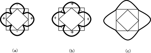
Figure 22: Evolution of the quasi-particle states when doping is reduced. (a) pure $d$ wave SC gap with nodal quasi-particles. (b) the pure $d$ wave SC gap is rotated into an AF gap of the form $|\cos p_{x}-\cos p_{y}|$. (c) A large uniform component of the AF/Mott insulating gap is developed on top of the $|\cos p_{x}-\cos p_{y}|$ gap when doping is reduced close to zero.

Because of the non-analyticity associated with the function $g({\bf p})$, this class of $SO(5)$ symmetric models contain long ranged interactions in real space. However, similar kinds of long ranged interactions are also present in the original BCS model due to the truncation of interactions in momentum space. Therefore, this class of $SO(5)$ models can be best viewed as low energy effective models resulting from integrating out states far from the Fermi surface. These models may address an important issue in the field of HTSC, which concerns the nature of the quasi-particle spectrum at the $d$ wave SC to AF transition. In the pure $d$ wave SC state, the SC order parameter is described by the form factor $d(p)=(\cos p_{x}-\cos p_{y})$. When the system is rotated into a uniform mixed AF/SC state, the form factor of the resulting AF order parameter is given by $g(p)d(p)=|\cos p_{x}-\cos p_{y}|$, which contains nodes at the same positions as in the pure $d$ wave SC state. When doping is further reduced, a uniform component of the AF gap develops across the Fermi surface, filling the $d$ wave nodes. This uniform AF gap gradually evolves into the AF Mott insulating gap at half-filling. See Fig. 22. Based on this scenario, Zacher et al Zacher et al. (2000) explained the $d$-wave like dispersion of the quasi-particle in the insulating stateRonning et al. (1998). Filling the $d$ nodes with the uniform AF gap also naturally explains the “small gap” observed in the photoemission experiments in the lightly doped cupratesShen and et al (2004). This theory of the quasi-particle evolution is also similar to the scenario of quantum disordering the nodal quasi-particles developed in Balents et al. (1998, 1999); Franz et al. (2002b); Herbut (2002). Recent studies have found that the generalized Hubbard model for spin 3/2 fermions enjoys an exact and generic $SO(5)$ symmetry without any fine tuning of model parameters and filling factors Wu et al. (2003a). Such a model can be accurately realized in systems of ultra-cold atoms on optical lattices, where the interaction is local and s wave scattering dominates Jaksch et al. (1998); Greiner (2002); Hofstetter et al. (2002). In the Hubbard model with spin 1/2 fermions, two fermions on the same site can only form a total spin $S_{T}=0$ state; the $S_{T}=1$ state is forbidden by the Pauli principle. Therefore, only one local interaction parameter specifies the on-site interaction. By a similar argument, two spin 3/2 fermions on the same site can only form the total spin $S_{T}=0,2$ states; the $S_{T}=1,3$ states are forbidden by the Pauli principle. Therefore, the generalized Hubbard model for spin 3/2 fermions is given by

$$H=-t\sum_{\langle ij\rangle,\sigma}\big{\{}c^{\dagger}_{i\sigma}c_{j\sigma}+h.c.\big{\}}-\mu\sum_{i\sigma}c^{\dagger}_{i\sigma}c_{i\sigma}$$

$$+U_{0}\sum_{i}P_{0}^{\dagger}(i)P_{0}(i)+U_{2}\sum_{i,m=\pm 2,\pm 1,0}P_{2m}^{\dagger}(i)P_{2m}(i),~{}~{}~{}$$ (106)

where $t$ is the hopping integral, $\mu$ is the chemical potential, and $P^{\dagger}_{0},P^{\dagger}_{2m}$ are the singlet ($S_{T}=0$) and quintet ($S_{T}=2$) pairing operators, defined as

$$P^{\dagger}_{0}(i)(P^{\dagger}_{20}(i))={1\over\sqrt{2}}\{c^{\dagger}_{3\over 2}c^{\dagger}_{-{3\over 2}}\mp c^{\dagger}_{1\over 2}c^{\dagger}_{-{1\over 2}}\},$$

$$P^{\dagger}_{2,2}(i)=c^{\dagger}_{3\over 2}c^{\dagger}_{1\over 2},\hskip 28.45274ptP^{\dagger}_{2,1}(i)=c^{\dagger}_{3\over 2}c^{\dagger}_{-{1\over 2}},$$

$$P^{\dagger}_{2,-1}(i)=c^{\dagger}_{1\over 2}c^{\dagger}_{-{3\over 2}},\hskip 14.22636ptP^{\dagger}_{2,-2}(i)=c^{\dagger}_{-{1\over 2}}c^{\dagger}_{-{3\over 2}}.$$ (107)

Remarkably, this generalized Hubbard model for spin 3/2 fermions is always $SO(5)$ symmetric, without any fine tuning of parameters and filling factors. This can be seen easily from the energy level diagram of a single site, which contains 16 states and 6 energy levels for spin 3/2 fermions, as depicted in Fig. 23. The $E_{1,4,6}$ levels are non-degenerate, the degeneracy of the $E_{2,5}$ levels is four-fold, and the degeneracy of the $E_{3}$ level is five-fold. We see that without any fine tuning of interaction parameters, this pattern of degeneracy exactly matches the singlet, the quartet (fundamental spinor) and the quintet (fundamental vector) representations of the $SO(5)$ group. It can also be easily verified that the hopping term also preserves the global $SO(5)$ symmetry. In fact, it preserves an even larger symmetry group, namely $SO(8)$. The $SO(8)$ symmetry is always broken by interactions; however, under special circumstances, its subgroups, $SO(7)$, $SO(6)$ and $SO(5)\times SU(2)$ can be realized in addition to the generic $SO(5)$ symmetry. In this article we mainly focus on application of the $SO(5)$ theory to the AF/SC systems. However, from the above discussions, we see that ultra-cold atoms on optical lattices also provide a fertile ground for investigating higher symmetries in strongly correlated systems, because the higher spins of the atoms and the accuracy of local interaction approximation. In the case of the spin 3/2 systems, the generic $SO(5)$ symmetry makes powerful predictions on the symmetries at quantum phase transition lines, spectrum degeneracies, topology of the ground state manifolds and low energy effective theories of the Goldstone bosons. With the emerging convergence between the atomic and condensed matter physics, we expect symmetry concepts and its multiple manifestations to play an ever increasing role in these fields.

Fermions in exact $SO(5)$ models have a beautiful non-abelian holonomy associated with themDemler and Zhang (1999a). The four components of an $SO(5)$ spinor represent four states but only two energy levels, each being doubly degenerate. As one varies some adiabatic parameters and returns to the same starting value, the states inside a doublet can be rotated into each other by a unitary transformation. This interesting mathematical property has been used to predict $SO(5)$ generalization of the Andreev effect and the non-abelian Aharonov-Bohm effectDemler and Zhang (1999a).

V.2 Variational wave functions

In this section we shall discuss a crucial test of the $SO(5)$ symmetry by investigating the microscopic wave functions of the $t-J$ model. In section IV.1, we showed that the transition from the AF state at half-filling to a pure $d$-wave SC state away from half-filling can generally be classified into three types. Within the general form of the static potential as given in Eq. (78), the “type 1” first order transition is realized for $u_{12}^{2}>u_{1}u_{2}$. For $u_{12}^{2}<u_{1}u_{2}$, the “type 2” transition involves two second order transitions with an intermediate mixed phase where the AF and the $d$-wave SC order coexist uniformly. Only for $u_{12}^{2}=u_{1}u_{2}$ is an intermediate “type 1.5” transition realized, where the potential can be re-scaled to take an $SO(5)$ symmetric form and a smooth rotation between the AF and the $d$-wave SC states is possible. If we only investigate states with uniform densities, these three possibilities can be distinguished easily by curvature in the plot of the ground state energy as a function of doping $\delta$. The curvature would be negative (concave), positive (convex), or zero (flat) for these three possibilities, as shown in Fig. (9). In the concave case, the uniform phase would be thermodynamically unstable, and a Maxwell’s construction leads to a phase separated ground state, where each phase has a distinct density.

This interesting prediction can be tested numerically in the $t-J$ model. At this moment, exact diagonalization of the $t-J$ model with large system size is not possible due to the exponential growth of the Hilbert space, and reliable Monte Carlo simulation cannot be carried out due to the fermion minus sign problem. A successful method employs the variational Quantum-Monte-Carlo (VMC) method (see, in particular, Gros (1989); Himeda and Ogata (1999); Calandra and Sorella (2000) and references therein). Historically, the VMC method was first used to investigate the RVB type of variational wave functions proposed by AndersonAnderson (1987). By investigating various variational wave functions, this method can address the issue of $d$-wave pairing in the ground state and the possibility of a uniform mixed phase with AF and $d$-wave SC order for the 2D $t-J$ model.

The first question is whether the uniform mixed state has a lower energy than the pure $d$-wave SC or AF state near half-filling. In earlier work by Zhang et al. Zhang et al. (1988) and by Yokoyama and Ogata Yokoyama and Ogata (1996), it was shown that the Gutzwiller approximation (GA) gives a reliable estimate for the variational energies for the pure $d$-wave SC state. However, if the AF order parameter is taken into account in the GA, there exists no region in the phase diagram where the AF state is stabilized. On the other hand, in Ref. Himeda and Ogata (1999), it was shown that when the variational parameters $\Delta_{d}$, $\Delta_{AF}$ and $\mu$ were determined from a VMC simulation, where the double occupancy prohibition is rigorously treated, then the Gutzwiller-projected trial wave function of the uniform mixed state has a lower energy than the pure $d$-wave SC state with $\Delta_{AF}=0$, in the doping range $0<\delta<10\%$. Using Green s-function Monte Carlo with stochastic reconfiguration (GFMCSR), Calandra and SorellaCalandra and Sorella (2000) also concluded that the AF correlations coexists with SC and persists up to $\delta=10\%$. Himeda and Ogata used the following Gutzwiller projected trial wave function:

$$\left|\psi\right>=P_{G}\left|\psi_{0}\left(\Delta_{\mathrm{d}},\Delta_{\mathrm{AF}},\mu\right)\right>\;,$$ (108)

where $\Delta_{d}$, $\Delta_{AF}$ and $\mu$ are the variational parameters relating to $d$-wave SC and AF order and $\mu$ is the chemical potential. $P_{G}=\prod_{i}\left(1-\hat{n}_{i\uparrow}\hat{n}_{i\downarrow}\right)$ stands for the Gutzwiller projection operator. The wave function $\left|\psi_{0}\left(\Delta_{\mathrm{d}},\Delta_{\mathrm{AF}},\mu\right)\right>$ is a mixed BCS/Spin-Density-Wave function, i. e.

$$\left|\psi_{0}\left(\Delta_{\mathrm{d}},\Delta_{\mathrm{af}},\mu\right)\right> = \prod_{k,s(=\pm)}\left(u^{(s)}_{k}+v^{(s)}_{k}d^{(s)\dagger}_{k\uparrow}d^{(s)\dagger}_{-k\downarrow}\right)\left|0\right>\;,$$ (109)

where the index $s=\left\{\pm\right\}$ takes care of the electron operators acting on the $A(B)$ sublattice in the AF state. The $u_{k}$’s and $v_{k}$’s contain the variational parameters $\Delta_{d}$, $\Delta_{AF}$ and $\mu$ and are defined in detail in Himeda and Ogata (1999). Fig. 24 is reproduced from this paper and plots the ground-state energy and the staggered magnetization as a function of doping $\delta$.

We see that in the Himeda and Ogata variational QMC work the uniform mixed phase of AF and $d$-wave SC has a lower energy than the pure $d$-wave SC state up to a doping of about 10%. At half-filling, the energy was found to be close to the best estimated value in the Green’s function MC method (-0.1994 to -0.20076), which provides support for the wave-function Ansatz Eq. (109) .

The second point of interest is that, according to the Himada and Ogata results in Fig. 24, the ground-state energy is a linear function of doping $\delta$ in this region, with essentially zero curvature. This implies that the chemical potential $\mu$ is constant. Since the wave function of Himada and Ogata describes a mixed state with uniform density, the energy versus doping plot can generally have three distinct possibilities, as enumerated in Fig. (9). Therefore, from the fact that the curvature is nearly flat we determine that the condition $u_{12}^{2}=u_{1}u_{2}$ is fulfilled, which places the $t-J$ model at $J/t=0.3$ into the domain of attraction of the $SO(5)$ fixed pointArrigoni and Hanke (2000); Murakami and Nagaosa (2000).

V.3 Exact diagonalization of the t-J and the Hubbard model

In the previous section we discussed the test of the $SO(5)$ symmetry through the variational wave functions in the $t-J$ model. In this section, we shall describe numerical calculations of the dynamic correlation functions and the exact diagonalization of the spectrum, which also tests the $SO(5)$ symmetry of the microscopic $t-J$ and Hubbard models. A microscopic model has a symmetry if its generators $G$ commute with the Hamiltonian $H$, i.e. $[H,G]=0$. In the $SO(5)$ theory, the $\pi_{\alpha}$ operators are the non-trivial generators of the symmetry. In models constructed in section V.1, the $\pi_{\alpha}$ operators indeed commute with the Hamiltonian. However, there are models where the symmetry generators do not commute with the Hamiltonian, but they satisfy a weaker condition, $[H,G^{\pm}]=\pm\lambda G^{\pm}$, where $\lambda$ is a $c$ number eigenvalue (see e.g. Eq. (22) in Section II). These operators are called eigen-operators of the Hamiltonian. In this case, from one eigenstate of the Hamiltonian, one can still generate a multiplet of eigenstates by the repeated actions of $G^{\pm}$. However, the eigenstates within a multiplet are not degenerate, but their energies are equally spaced by $\lambda$. A classic example is the precession of a spin in a magnetic field, where

$$H=\omega_{0}S_{z};\quad\quad[H,S_{\pm}]=\pm\omega_{0}S_{\pm}\,.$$ (110)

and $\omega_{0}$ is the Lamor frequency of the spin precession. Although in this case the spin-rotational symmetry is broken explicitly by the magnetic field in the $z$-direction and the eigenstates within the multiplets are no longer degenerate, the multiplet structure of the symmetry is still visible in the spectrum and can be sampled by the ladder operators. If one calculates the dynamical response function of $S_{\pm}$, only a single $\delta$-peak is present at $\omega=\omega_{0}$.

The $\pi_{\alpha}$ operators defined in equation (44) do not commute with the Hubbard or $t-J$ model Hamiltonian, but analytical and numerical calculations show that they are approximate eigen-operators of these model, in the sense that

$$[H,\pi^{\dagger}_{\alpha}]\approx\omega_{\pi}\pi^{\dagger}_{\alpha}$$ (111)

is satisfied in the low energy sector. This means that the dynamic auto-correlation function of the $\pi_{\alpha}$ operators contains a sharp pole at $\omega_{\pi}$, with broad spectral weight possibly istributed at higher energies. Using a T-matrix approximation, Demler and Zhang Demler and Zhang (1995) verified this approximate equation with $\omega_{\pi}=J(1-n)/2-2\mu$. This calculation will be reviewed in section VI.4. The first numerical test for a low-energy $SO(5)$ symmetry in a microscopic model has been performed by Meixner et al. Meixner et al. (1997) using the Lanczos Lanczos (1950) exact diagonalization technique. Analysis presented in this paper showed that the dynamical correlation function of the $\pi$-operator

$$\pi^{\dagger}_{\alpha}(\omega)=-\frac{1}{\pi}{\rm Im}\langle\Psi_{0}^{N}|\pi_{\alpha}\frac{1}{\omega-H+E_{0}^{N+2}+i\eta}\pi_{\alpha}^{\dagger}|\Psi_{0}^{N}\rangle.$$ (112)

(with $H$ being the standard Hubbard Hamiltonian, $|\Psi_{0}^{N}\rangle$ its ground state with $N$ electrons and $E_{0}^{N}$ the corresponding ground state energy) yielded a single sharp excitation peak at low energy $\omega_{\pi}$, accompanied by an incoherent background at higher energies. The large separation between the peak and the continuum and the large relative spectral weight of the peak demonstrated that indeed the $\pi$-operator is an approximate eigenoperator of the Hamiltonian (see Fig. 25). Also in accordance with the perturbative result of Ref.Demler and Zhang (1995), the “precession frequency” $\omega_{\pi}$ decreases for decreased doping. Furthermore, a comparison with a bubble approximation for this correlation function showed that the sharp peak near $\omega_{\pi}$ originated solely from vertex corrections (i.e. collective behavior).

Not only can the dynamic correlation function of the $\pi_{\alpha}$ operators (112) be measured numerically for microscopic models, thus providing a test of the approximate $SO(5)$ symmetry, but they can also be directly measured in neutron scattering experiments in the SC state. We shall discuss these experiments in section VI.

Exact numerical diagonalization of the $t-J$ and Hubbard models gives eigenstates and eigenvalues on a finite size cluster, whose degeneracy pattern can be used directly to test the $SO(5)$ symmetry. In order to explain the main idea, let us first examine the variational wave function of the projected $SO(5)$ model given in Eq. (74). This wave function describes a broken symmetry state formed by a linear superposition of states with different spin or charge quantum numbers. This type of state can only be realized in infinite systems. On a finite size system, all eigenstates must have definite spin and charge quantum numbers. Denoting $t^{\dagger}(x)=m_{\alpha}(x)t^{\dagger}_{\alpha}(x)+\Delta(x)t^{\dagger}_{h}(x)$, we can expand the coherent state described by Eq. (74) as

$$|\Psi\rangle=\{\cos\theta^{N}+\cos\theta^{N-1}\sin\theta\sum_{x}t^{\dagger}(x)+\cos\theta^{N-2}\sin\theta^{2}\sum_{x\neq y}t^{\dagger}(x)t^{\dagger}(y)+\cos\theta^{N-3}\sin\theta^{3}\sum_{x\neq y\neq z}t^{\dagger}(x)t^{\dagger}(y)t^{\dagger}(z)+...\}|\Omega\rangle.$$ (113)

For $\Delta(x)=0$, we see that the AF ordered state can be expressed as a linear superposition of states with different numbers of magnons, forming states with different total spins. While states with different total spins are separated by finite energy gaps in a finite size system, these energy gaps could vanish in the thermodynamic limit, allowing magnons to “condense” into the ground state. For $m_{\alpha}(x)=0$, we see that the SC state can be expressed as a linear superposition of states with different numbers of hole pairs, with different total charge. A smooth rotation from the AF state to the SC state becomes possible if one can freely substitute each magnon by a hole pair without energy cost. This places a powerful requirement on the spectrum. The $\sum_{x}t^{\dagger}(x)|\Omega\rangle$ term in (113) contains a single magnon state with ($S=1$, $Q=0$) or a single hole pair state with ($S=0$, $Q=-1$). $SO(5)$ symmetry requires them to be degenerate. This can be easily achieved by tuning the chemical potential, which changes the energy of the hole pair state without changing the energy of the magnon state. Once the chemical potential is fixed, there are no additional tuning parameters. The $\sum_{x\neq y}t^{\dagger}(x)t^{\dagger}(y)|\Omega\rangle$ term in (113) contains a two-magnon state with ($S=2$, $Q=0$), a one-magnon-one-hole-pair state with ($S=1$, $Q=-1$) and a two-hole-pair state with ($S=0$, $Q=-2$). $SO(5)$ symmetry again requires them to be degenerate, which is a highly non-trivial test. We can easily perform this analysis for states with different numbers of magnons and hole pairs.

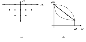
Figure 26: After expanding out the coherent state (74), we obtain the magnon and hole pair states at level $\nu$, which is the total number of magnons and hole pairs. These states are classified by their $(S_{z},Q)$ quantum numbers in (a). The energy is independent of the $S_{z}$ quantum number because of the $SO(3)$ spin rotation symmetry. The energy can depend on $Q$ with three generic possibilities, as depicted in (b). (Compare with Fig. 9). If the energy depends linearly on $Q$, there is no free energy cost to rotate magnons and hole pairs into each other, and the potential energy is $SO(5)$ symmetric. This multiplet structure was tested in the $t-J$ model and shown in Fig. 27.

This pattern of the energy levels has been tested directly in the exact diagonalization of the $t-J$ model by Eder, Hanke and Zhang Eder et al. (1998). The $t$$-$$J$ model, because of its more limited Hilbert space (no double occupancies), allows the exact diagonalization of larger systems (18, 20 and more sites). Since the $t$$-$$J$ model explicitly projects out the states in the upper Hubbard band, some of the questions about the compatibility between the Mott-Hubbard gap and $SO(5)$ symmetry can also be answered explicitly. In the exact diagonalization studies, total energy, momentum, angular momentum, spin and the charge quantum numbers of the low energy states can be determined explicitly. These quantum numbers are summarized in Fig. (26)a.

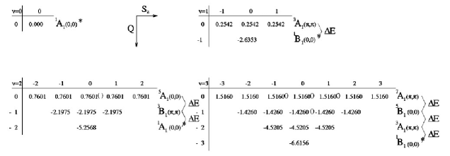
Figure 27: The low energy states within each total spin and charge sector $(S_{z},Q)$ of the $18$-site cluster $t-J$ model with $J/t=0.5$. The states are grouped into different multiplets and are labelled by the spin, charge, point group symmetry, and total momentum. $A_{1}$ denotes the totally symmetric, $B_{1}$ the $d_{x^{2}-y^{2}}$-like representation of the $C_{4v}$ symmetry group. The quantum numbers of these states match that of the magnon and hole pair states shown in Fig. 26. Furthermore, the energy depends approximately linearly on $Q$, demonstrating the $SO(5)$ symmetry of the interaction potential among the magnons and hole pairs.

Eigenstates obtained from the $t-J$ or Hubbard Hamiltonian can always be interpreted as multi-particles states of the underlying electron. However, it would be highly non-trivial if the low energy states could also be interpreted as multi-particle states formed from the collective degrees of freedom such as the magnons and the hole pairs. The first non-trivial finding of Ref. Eder et al. (1998) is that this is indeed the case. Fig. 27 shows the first four $(\nu=0$ to $\nu=3)$ sets of low-lying states of an 18-site $t-J$ model Eder et al. (1998). We see that the lowest energy state in the $S=1,Q=0$ sector indeed has $s$ wave like rotational symmetry and total momentum $(\pi,\pi)$, as expected from a magnon; the lowest energy state in the $S=0,Q=-1$ sector indeed has a $d$-wave like rotational symmetry and total momentum $0$. Similarly, states with higher $S$ and $Q$ have quantum numbers expected from multiple magnons and hole pairs. This finding confirms the basic assumption of the $SO(5)$ theory, that the low energy collective degrees of freedom can be described by the superspin alone.

At the next level, the pattern of symmetry can itself be tested. The level $\nu$ of a given multiplet indicates the total number of magnons and hole pairs. If $SO(5)$ symmetry is realized at a given chemical potential $\mu_{c}$, we would expect the free energy to depend only on $\nu$, the total number of magnons and hole pairs, but not on the difference between the number of magnons and hole pairs. As shown in Fig. 26, the energy can depend on $Q$ with three generic possibilities, similar to the discussions we presented in section IV.1 and Fig. 9. Only when the energy depends linearly on $Q$ can the free energy be independent of $Q$ at a given critical value of the chemical potential. From (27) we see that the energy levels indeed have this remarkable structure: states whose total charge differ by $\Delta Q=-1$ have nearly the same difference in energy. Therefore, the energy is approximately a linear function of $Q$ or doping, similar to the situation discussed in section V.2. To be more precise, the mean-level spacing within each multiplet (up to $Q=-2$) is $-2.9886$ with a standard deviation of $0.0769$. This standard deviation is much smaller $\left(\sim J/8\right)$ than the natural energy scale $J$ of the $t$$-$$J$ model and comparable to or even smaller than the average SC gap. Therefore, if one now adds the chemical potential term $H_{\mu}=-2\mu Q$, and chooses $\mu=\mu_{c}$ equal to the mean-level spacing, the superspin multiplets are nearly degenerate. At $\mu=\mu_{c}$, magnons can be smoothly converted into hole pairs without free energy cost. This means that in each term of the expansion in (113) one can freely substitute $t^{\dagger}_{\alpha}$ or $t^{\dagger}_{h}$ for $t^{\dagger}$, and the direction of the superspin vector can be freely rotated from the AF to the SC direction. The smallness of the standard deviation indicates the flatness in the energy versus doping plot discussed in the previous section. If the standard deviation is significantly different from zero, this would indicate significant curvature in the energy versus doping plot. Therefore, the smallness of the standard deviation obtained by the exact diagonalization is consistent with the flatness of the energy versus doping plot obtained from the variational wave function discussed in the previous section.

Another important aspect of the $SO(5)$ symmetry is the Wigner-Eckart theorem Georgi (1982). This theorem provides a selection rule for the matrix elements of the operators based on the $SO(5)$ symmetry of the system. It implies, for example, that the $\pi$ operators (see equation (44)) can only move us within a given multiplet, since they are symmetry generators. On the other hand, AF and $d$-wave SC order parameters (see equations (42)) should move us between different multiplets. Both features have been verified in the numerical calculations in Eder et al. (1998).

We conclude this subsection with a general remark. Exact diagonalizations (e.g. Dagotto (1994)) commonly study ground-state correlations, but their spatial decay is often inconclusive as a test of order due to small system size. Discussions in this section show that it is possible that the (excited) eigenstates reveal a well-defined structure characteristic of a particular symmetry. Our strategy is to use the finite size calculations as input for effective models describing the collective degrees of freedom such as the superspin, or the magnons and the hole pairs. Since quantum Monte Carlo calculations can be performed for these models in a large size systems, the question of long range order and their competition can be firmly established.

V.4 Transformation from the microscopic model to effective SO(5) models

From the two previous sections we have learned that both the variational wave function and the exact diagonalization of the $t-J$ model show that the ground state and low lying excited states in the low doping range can be completely described in terms of the superspin degree of freedom, with an approximate $SO(5)$ symmetry. Altman and AuerbachAltman and Auerbach (2002) pioneered a systematic procedure in which they derived the effective bosonic $SO(5)$ model directly from the microscopic Hubbard and $t-J$ models through a renormalization group transformation called the Contractor Renormalization (“CORE”) methodMorningstar and Weinstein (1996). This mapping has several distinct advantages. First, this approach helps to visualize clearly which processes and which excitations dominate the low energy physics of the system. Second, their work directly determines the parameters of the effective models defined in Eq. (69) and (84) in terms of the microscopic parameters. The bosonic systems are often much easier to analyze numerically, as one does not have to worry about Pauli principles, Slater determinants, and the infamous sign problem in the quantum Monte Carlo algorithms. In this section, we shall describe their work.

Since we want to construct bosonic quasiparticles, we have to divide the lattice into effective sites containing an even number of elementary sites (with one electron per site). In order to conserve the symmetry between the $x$ and $y$-direction in the system, the original projected $SO(5)$ model was formulated on a plaquette of $2\!\times\!2$ elementary sites. First we begin with the low energy eigenstates of the Heisenberg plaquette, which are determined easily. We find the nondegenerate ground state $|\Omega\rangle$ (see Fig. 6 for a real-space representation in terms of the microscopic states on a plaquette) with energy $E_{0}\!=\!-2J$ and total spin $S\!=\!0$. This singlet state will be the vacuum state of the effective bosonic projected $SO(5)$ model. The next energy eigenstates are three triplet states $t^{\dagger}_{\alpha}|\Omega\rangle$ with energy $E_{t}\!=\!-J$ and spin quantum numbers of $S\!=\!1$. All other energy eigenstates of the Heisenberg plaquette have higher energies and can be neglected in the low energy effective model. It should be noted that the quasiparticles $t_{\alpha}$, which carry spin 1 and charge 0, are hardcore bosons because one cannot create more than one of them simultaneously on a single plaquette.

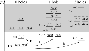
Figure 28: Low energy spectrum of the Hubbard model on a plaquette. Eigenstates by total spin $S$ and plaquette momentum $q_{x},q_{y}=0,\pi$. Truncated high energy states are shaded. The vacuum is defined as $|\!\;{{\Omega}}\!\;\rangle$, and quantized operators connect the vacuum to the lowest eigenstates as shown. (In this figure, $t^{\dagger}$ denotes the magnon creation operator $t_{\alpha}^{\dagger}$, and $b^{\dagger}$ denotes the hole pair creation operator $t_{h}^{\dagger}$.)

In their CORE study of the 2D Hubbard model, Altman and Auerbach Altman and Auerbach (2002) started from the spectrum of lowest-energy eigenstates of the 2 x 2 plaquette for 0, 1 and 2 holes, respectively. The corresponding lowest spectrum of the triplet $(t_{\alpha}^{\dagger})$, pair boson $(t_{h}^{\dagger})$ and fermionic excitations is presented in Fig. 28. The ground state of two holes, also depicted in Fig. 6, is described by

$$t_{h}^{\dagger}\left|\Omega\right>=\frac{1}{\sqrt{Z_{b}}}\left(\sum_{ij}d_{ij}c_{i\uparrow}c_{j\downarrow}+\ldots\right)\left|\Omega\right>,$$ (114)

where $d_{ji}$ is +1 (-1) on vertical (horizontal) bonds within a plaquette and $\ldots$ stands for higher-order (U/t)-operators. $Z_{b}$ is the wavefunction normalization. We note that $t_{h}^{\dagger}$ creates a “Cooper”-like hole pair with internal $d$-wave symmetry with respect to the vacuum. The crucial point here is that while there is no hole pair binding for the Hubbard model on a dimer, there is binding in the range of $U/t\in(0,5)$ for a plaquette, a rather well-known fact (see, for instance, Ref.Hirsch et al. (1988)). However, this does not guarantee the integrity of the pair binding on the infinity lattice, documented by the fact that the hopping energy $t$ is much larger than the pair binding energy, nor does it guarantee long-range SC order. To get more insight into these questions, one has to construct $H_{eff}$ via a CORE procedure.

In order to understand how the triplets and pair bosons behave on the infinite lattice, we must determine the boson hopping energies and the corresponding effective Hamiltonian. A suitable approach for this has been suggested by Morningstar and Weinstein on the basis of the CORE technique, which has been shown for the 2D Hubbard model Altman and Auerbach (2002), $t-J$ ladders Capponi and Poilblanc (2002) and earlier for Heisenberg chains and ladders Morningstar and Weinstein (1996) to be extremely accurate. For example, Morningstar and Weinstein obtained a very accurate 1D Heisenberg model ground-state energy. This is even more impressive considering the latter model has long-range, power-law decaying spin correlations.

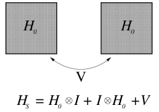
Figure 30: This figure illustrates the construction of the “superblock” and its Hamiltonian $H_{s}$ out of two neighboring blocks, with intrablock Hamiltonian $H_{0}$ and interblock coupling V (in the block basis: $\left(H_{0}\right)_{n,n^{\prime}}=\langle\alpha_{n}^{\circ}\mid H\mid\alpha_{n}^{\circ}\rangle=\epsilon_{n}^{\circ}\delta_{n,n^{\prime}}$ and $\left(V_{0}\right)_{nm,n^{\prime}m^{\prime}}=\langle\alpha_{n}^{\circ}\alpha_{m}^{\circ}\mid V\mid\alpha_{n^{\prime}}^{\circ}\alpha_{m^{\prime}}^{\circ}\rangle$).

In order to implement the CORE technique, the lattice is decomposed in small block units, as shown in Fig. 30, where $H_{0}$ is the intra-block Hamiltonian and $V$ is the part describing the coupling between the two neighboring blocks. The $M$ low-energy states $\{|\alpha^{0}\rangle\}_{i}^{M}$ are kept in each block $i$ (here $M=4$ in the $2\times 2$ plaquette $i$) to define a reduced Hilbert space. The full Hamiltonian is then diagonalized on $N$ connected units (in our example in Fig. 30, $N=2)$, i. e. for the (superblock) Hamiltonian $H_{S}$. The $M^{N}$ (in our case, $M^{N}=4^{2}$) lowest energy states $|\Psi_{n}\rangle$ with energy $\epsilon_{n}$, $n=1\ldots M^{N}$ are retained. These true eigenstates of the $N(=2)$ block problem, $\{|\Psi_{n}\rangle\}$, are then projected onto the reduced Hilbert space spanned by the tensorial product $|\alpha^{0}_{1}\ldots\alpha^{0}_{N}\rangle$ of the $M(=4)$ states of each block, i. e.

$$\left|\Psi^{\prime}_{n}\right>=\sum_{\alpha_{1}\ldots\alpha_{N}}\left<\alpha^{0}_{1}\ldots\alpha^{0}_{N}\mid\Psi_{n}\right>\left|\alpha^{0}_{1}\ldots\alpha^{0}_{N}\right>,$$ (115)

and Gram-Schmidt orthonormalized, finally yielding the states $\{|\tilde{\Psi}_{n}\rangle\}$. Then, the new superblock (renormalized) Hamiltonian is defined as

$$\tilde{H}_{S}=\sum^{M^{N}}_{n}\epsilon_{n}\left|\tilde{\Psi}_{n}\right>\left<\tilde{\Psi}_{n}\right|.$$ (116)

By construction $\tilde{H}_{S}$, has the same eigenvalues $\epsilon_{n}$ as $H_{S}$ for $n=1,\ldots,M^{N}$. Having constructed the new superblock or renormalized Hamitonian $\tilde{H}_{S}$, one can write (in our $N=2$ example)

$$\tilde{H}_{S}=\tilde{H}_{0}\otimes\mathrm{I}+\mathrm{I}\otimes\tilde{H}_{0}+\tilde{V},$$ (117)

where $\tilde{H}_{0}$ is simply the projected block Hamiltonian:

$$\tilde{H}_{0}=\sum^{M}_{n=1}\epsilon_{n}\left|\alpha^{0}_{n}\right>\left<\alpha^{0}_{n}\right|.$$ (118)

The above equation (117) gives the new renormalized interblock coupling $\tilde{V}$, restricted to the reduced Hilbert space. In the next step, one repeats the above procedure, replacing $H_{0}$ and $V$ in the original superblock Hamiltonian $H_{S}$ by $\tilde{H}_{0}$ and $\tilde{V}$, and so on.

The projection onto the original plaquette product basis in the Eq. (115) expresses, of course, the above-discussed proliferation and possibly spatial decay of the block excitations. More generally, this is incorporated within the CORE method, in a superblock consisting of $N$ blocks and a corresponding Hamiltonian containing $N$-body interactions. The construction to obtain $\tilde{V}$ (Eq. (117)) is different and, obviously, one also obtains $\tilde{V}$-terms, connecting $N$ clusters instead of just $N=2$ (called range-$N$-approximation). It has been shown in the above-cited various applications that the above range-2 approximation ($N=2$) and at most $N=3$ interactions already yield very accurate results. Thus, with a proper and physically motivated choice of the truncated basis, range-N interactions decay rapidly with $N$.

In Ref. Altman and Auerbach (2002), the CORE calculation was limited to range-2 boson (triplets, hole pair boson) interactions leaving out the fermion state. From the above Fig. 30, i. e. it is clear that this amounts to diagonalizing two coupled ($2\times 2$) plaquettes, for instance, an 8-site Hubbard cluster, which is very straightforward by the Lanczos technique. The resulting effective Hamiltonian for this range-2 four-boson model is exactly the projected $SO(5)$ model defined in Eq. (69) plus more extended interactions defined in Eq. (84). Following Altman and Auerbach, we compare in Fig. 31 the magnitudes of the magnon hopping $J_{s}$ (denoted as $J_{t}/2\simeq J_{tt}/2$ in Ref. Altman and Auerbach (2002)) and the hole pair hopping $J_{c}$ (denoted as $J_{b}$ in Ref. Altman and Auerbach (2002)) for a range of $(U/t)$-values.

The first observation is that $J_{t}\sim J_{tt}\sim 0.6J$; therefore, the triplet terms have a similar magnitude as those previously (see also our simple pedagogical Heisenberg example) obtained Sachdev and Bhatt (1990); Gopalan et al. (1994).

The second finding is crucial. The region of equal $J_{t}$ $(J_{tt})$ and $J_{b}$, equal magnon- and pair-boson hopping, occurs very close to $U/t=8$. Thus, the value of the projected $SO(5)$ model with $J_{t}=J_{b}$ occurs in the physically relevant regime: It is known from a large body of numerically essentially exact (for example QMC) evaluations of the 2D Hubbard model that it reproduces salient features of the HTSC cuprates precisely in this regime (see for example Dagotto (1994); Imada et al. (1998). This gives yet another piece of evidence, in addition to those discussed in sections V.2 and V.3, that realistic microscopic models can be described effectively by the projected $SO(5)$ model close to the symmetric point.

Altman and AuerbachAltman and Auerbach (2002), Capponi and PoilblancCapponi and Poilblanc (2002) also calculated the coefficient and terms on $H^{int}$ in Eq. (84), which contains triplet-triplet, pair-pair and pair-triplet interactions. These interaction terms were found to be small compared to $H^{b}$ and $H^{t}$, but their influence has yet to be studied in detail. They also estimated the truncation error of discarding range-3 terms which, for physically relevant $U$-values, was found to be very small (1%).

An issue still left open is the role of fermions. Altman and Auerbach have extended the above 4-boson model to a boson-fermion model by augmenting the bosons with single-hole fermions “by hand.” This is certainly a first step. However, a consistent low-energy theory has to treat bosons and fermions within the CORE procedure on equal footings. It should, however, be noted that the short-range effects of the fermions on the effective boson couplings were included in the above range-2 calculation. Altman and Auerbach estimated the fermion-boson interaction by including the hole fermions dispersion “adhoc”, i. e. using the single-hole band-structure extracted previously by various groups for large clusters Dagotto (1994).

In summary, the application of the CORE algorithm to the Hubbard model has demonstrated two features which are of immediate relevance for the $SO(5)$ theory: the $d$-wave hole pairs already present in the 2D Hubbard model on a single 2 x 2 plaquette maintain their integrity in the “infinite” square lattice. The low energy degrees of freedom are indeed described solely by the superspin. Secondly, the hole-pair and magnon (triplet) hopping fulfills the projected $SO(5)$ condition in the physically relevant (U/t)-range.

VI PHYSICS OF THE $\pi$ RESONANCE AND THE MICROSCOPIC MECHANISM OF SUPERCONDUCTIVITY

A key experimental manifestation of a higher symmetry is the emergence of new particles or new collective modes. Historically, this line of reasoning has led to important discoveries in particle physics. For example, Gell-Mann used the $SU(3)$ symmetry of the strong interaction to predict the $\Omega^{-}$ resonance. Similarly, the electro-weak unification based on the $SU(2)\times U(1)$ symmetry has led to the prediction of the $W^{\pm}$ and the $Z$ bosons. In a strongly interacting system, whether in particle physics or in condensed matter physics, typical excitations have short life times and broad line shapes. However, if higher symmetries are present, the selection rules associated with the symmetry prevents the excitation from decaying. The $SO(5)$ symmetry of antiferromagnetism and superconductivity naturally predicts a new class of collective excitations, called the $\pi$ resonance or $\pi$ mode for short, which are the (pseudo-) Goldstone modes of the spontaneous symmetry breaking. The $\pi$ resonance can be identified naturally with the neutron resonance observed in the HTSC cuprates Rossat-Mignod et al. (1991a); Mook et al. (1993); Fong et al. (1995). In this section we will review basic experimental facts about such resonances and discuss a theoretical scenario in which they originate from the pseudo Goldstone modes associated with the $SO(5)$ symmetry. The operator of the $\pi$-mode is a symmetry generator of the $SO(5)$ symmetry, so the appearance of the low lying resonance tells us about a small energy difference between the $d$-wave SC and AF ground states of the doped cuprates. The idea of the near degeneracy of the $d$-wave SC and AF states lies at the heart of the $SO(5)$ approach, which assumes that fluctuations between these two states exhaust the low energy sector of the system. Hence, experimental observation of the low lying resonances provide a key foundation to the $SO(5)$ approach to competing AF and SC in the cuprates. In this section we provide several perspectives on the $\pi$-excitations. First, we use the $SO(5)$ non-linear sigma model to describe them as pseudo-Goldstone modes of the approximate $SO(5)$ symmetry of the system. Second, we show that the Fermi liquid analysis of the weakly interacting electron gas in a two dimensional tight binding lattice produces the $\pi$-mode as a sharp collective mode and gives a simple picture of this excitation as an anti-bound state of two electrons with the total spin $S=1$ and with the center of mass momentum $\Pi=(\pi,\pi)$. Such excitation contributes to the spin fluctuation spectrum, measured by the inelastic neutron scattering, only in the SC state when there is a condensate of Cooper pairs. Finally, we discuss an important role that the $\pi$-resonance plays in stabilizing the SC state.

VI.1 Key experimental facts

Resonant peak in the SC state of the cuprates was first observed in optimally doped $YBa_{2}Cu_{3}O_{7}$ Rossat-Mignod et al. (1991a, b, 1992). Further experiments Mook et al. (1993); Fong et al. (1995) established that this is a magnetic resonance (spin $S=1$) at the AF wavevector $\Pi=(\pi,\pi)$ which appears in the SC state. It has a constant energy $\omega_{0}=41~{}{\rm meV}$ at all temperatures and intensity that is strongly temperature dependent and vanishes at $T_{c}$. Similar resonances have then been found in underdoped $YBa_{2}Cu_{3}O_{6+x}$ Dai et al. (1996); Fong et al. (1996); Mook et al. (1998); Dai et al. (1998); Fong et al. (2000); Stock et al. (2003) and in $Bi_{2}Sr_{2}CaCu_{2}O_{8+\delta}$ Fong et al. (1999); He et al. (2001) and $Tl_{2}Ba_{2}CuO_{6+\delta}$ He et al. (2002).

An important feature of magnetic scattering in underdoped $YBa_{2}Cu_{3}O_{6+x}$ Dai et al. (1996, 1998); Mook et al. (1998); Fong et al. (2000) is that the resonance precursors are detectable above $T_{c}$. Magnetic correlations, however, are strongly enhanced in the SC state, and there is a cusp in the temperature dependence of the resonant scattering intensity at $T_{c}$ Fong et al. (2000). Doping dependence of the resonance energy and intensity indicate a strong enhancement of magnetic fluctuations as we approach half-filling: for underdoped $YBa_{2}Cu_{3}O_{6+x}$ the resonance energy decreases with decreasing doping, and the intensity increases Fong et al. (2000). For overdoped $Bi_{2}Sr_{2}CaCu_{2}O_{8+\delta}$ it was found that the energy decreased He et al. (2001, 2002), which led to a suggestion that the resonance energy follows the SC transition temperature He et al. (2001).

The presence of the magnetic resonance in the SC state of many cuprates suggests that it is closely related to the SC pairing. This idea was reenforced by the experiments of Dai et.al Dai et al. (2000), in which the SC coherence in $YBa_{2}Cu_{3}O_{6.6}$ was suppressed by applying a magnetic field. It was found that the resonance intensity decreased without any noticeable change in the resonance energy. Finally, in Dai et al. (1999) it was demonstrated that the exchange energy associated with the resonance has the right magnitude, the temperature and doping dependences to describe the SC condensation energy of $YBa_{2}Cu_{3}O_{6+x}$ materials.

VI.2 Contribution of the $\pi$ resonance to the spin correlation function

Resonance that appears in the SC state suggests that what gets scattered is Cooper pairs which are only present below $T_{c}$. Based on this idea it was proposed Demler and Zhang (1995) that the resonance observed in inelastic neutron scattering experiments is due to the presence of the $\pi$-mode, a sharp collective mode in the particle-particle channel at momentum $\Pi=(\pi,\pi)$ with spin $S=1$. In the normal state such excitation does not contribute to the magnetic spectrum, since the latter is determined by fluctuations in the particle-hole channel. Below $T_{c}$, on the other hand, condensed Cooper pairs couple the particle-hole and particle-particle channels Demler and Zhang (1995); Demler et al. (1998b) and cause the $\pi$ excitation to appear as a sharp resonance in the magnetic spectrum with intensity set by the strength of mixing of the two channels, $|\Delta(T)|^{2}$, where $\Delta(T)$ is the amplitude of the SC order parameter. Such a scenario provides a natural explanation for the key properties of the observed resonance: its energy is essentially the energy of the $\pi$ mode in the normal state and is temperature independent Demler et al. (1998b), whereas the intensity of the resonance is set by $|\Delta(T)|^{2}$ and vanishes at $T_{c}$.

Coupling of the particle-particle $\pi$-channel and the particle-hole AF channel may be understood using the commutation relations between the operators $\pi_{\alpha}$ and $N_{\beta}$ given in equation (27). In the SC state the $d$-wave SC order parameter that enters the right hand side of equation (27) can be replaced by its expectation value in the ground state. Hence, the commutator of $\pi$ and $N$ becomes a ${\rm c}$-number, and the two fields become conjugate variables, just as coordinate and momentum are conjugate to each other in elementary quantum mechanics. The result of such coupling is that the $\pi$-mode appears as a sharp resonance in the spin fluctuation spectrum. To demonstrate this we consider the spin-spin correlation function at wavevector $\Pi$

$$\chi(\Pi,\omega)=-i\int e^{-i\omega t}\langle TN_{\alpha}(t)N_{\alpha}(0)\rangle dt=\sum_{n}|\langle n|N_{\alpha}|0\rangle|^{2}\left\{\frac{1}{\omega-E_{n}+i0}-\frac{1}{\omega+E_{n}-i0}\right\}.$$ (119)

Here $|0\rangle$ is the ground state and $n$-summation goes over all excited states of the system. One of the excited states is created by the $\pi$-operator defined in equation (44)

$$|\pi_{\alpha}\rangle=\frac{1}{{\cal N}}\pi_{\alpha}^{\dagger}|0\rangle,$$ (120)

where ${\cal N}$ is the normalization factor.

It is useful to realize that if $\pi^{\dagger}$ acting on the ground state creates an excited state, then $\pi$ should annihilate it (otherwise it would create a state of lower energy than the ground state Pines and Nozieres (1966)). Then we have

$$1=\langle\pi_{\alpha}|\pi_{\alpha}\rangle=\frac{1}{{\cal N}^{2}}\langle 0|\pi_{\alpha}\pi_{\alpha}^{\dagger}|0\rangle=\frac{1}{{\cal N}^{2}}\langle 0|\left[\pi_{\alpha},\pi_{\alpha}^{\dagger}\right]|0\rangle\approx\frac{(1-n)}{{\cal N}^{2}},$$ (121)

where $n$ is the filling fraction ($n=1$ corresponds to half-filling). In writing the last equality we assumed $\langle(g(p))^{2}\rangle=1$ when averaged around the Fermi surface.

If we separate the contribution of the $\pi$ state to $\chi(\Pi,\omega)$ we have

$$\chi(\Pi,\omega)=|\langle\pi_{\alpha}|N_{\alpha}|0\rangle|^{2}\frac{1}{(\omega-\omega_{\pi}+i0)}+{\rm part\;regular\;at\;\omega_{\pi}}.$$ (122)

The resonant contribution to $\chi(\Pi,\omega)$ can be expressed as

$$\chi^{\rm res}(\Pi,\omega) = \frac{1}{{\cal N}^{2}}|\langle 0|\pi_{\alpha}N_{\alpha}|0\rangle|^{2}\frac{1}{(\omega-\omega_{\pi}+i0)}=\frac{1}{{\cal N}^{2}}|\langle 0|\left[\pi,N\right]|0\rangle|^{2}\frac{1}{(\omega-\omega_{\pi}+i0)}$$ (123)

$$\approx \frac{|\langle 0|\Delta|0\rangle|^{2}}{(1-n)}\frac{1}{(\omega-\omega_{\pi}+i0)}.$$

The expectation value in the numerator of the last expression is simply the amplitude of the superonducting $d$-wave order parameter. We emphasize that Eq. (123) does not rely on the details of the microscopic model but only on the commutation relations between the $\pi$, $N$, and $\Delta$ given by the equation (27) (this is somewhat analogous to the $f$-sum rule Pines and Nozieres (1966)). To relate the order parameter to what one typically measures in experiments we use BCS type arguments to connect the order parameter to the quasiparticle gap (see however Uemura et al. (1989); Emery and Kivelson (1995)) $\langle 0|\Delta|0\rangle=C\Delta_{0}/V_{BCS}$. Here $\Delta_{0}$ is the maximal gap for Bogoliubov quasiparticles at the antinodal point, $V_{BCS}$ is the interaction strength that we expect to be of the order of the nearest-neighbor exchange coupling $J$, and $C$ is a dimensionless constant of the order of unity. Therefore, we find

$$\chi^{\rm res}(\Pi,\omega)=C^{2}\,\,\frac{|\Delta_{0}|^{2}}{J^{2}(1-n)}\frac{1}{\omega-\omega_{\pi}+i0}.$$ (124)

As we go to the underdoped regime, $\Delta_{0}$ remains constant or increases slightly, and the factor $1-n$ decreases. Eq. (124) predicts that the intensity of the resonance should increase; this increase has been observed in the experiments in Ref. Fong et al. (2000).

It is useful to note that contributions from modes other than the $\pi$ excitation do not spoil the result in (123). If most of the $\pi$-spectrum is accommodated in an interval $(\omega_{\pi}-\nu,\omega_{\pi}+\nu^{\prime})$, one can use the Cauchy-Schwarz inequality to prove a rigorous and model-independent resultDemler et al. (1998b) that

$$\frac{1}{\pi}\int_{\omega_{\pi}-\nu}^{\omega_{\pi}+\nu^{\prime}}d\omega{\rm Im}\chi^{\rm res}(\Pi,\omega)\geq\frac{|\Delta|^{2}}{1-n}.$$ (125)

The left hand side of this equation represents the contribution of the $\pi$ mode to the spin excitation spectrum and the right hand side gives its lower bound. Exact equality holds when $\pi$ operator is an exact eigenoperator and hence there is only one energy eigenstate which satisfies $\langle 0|\pi_{\alpha}|n\rangle\neq 0$.

Thus, a simple picture of the resonant neutron scattering is as follows: when an incoming neutron is scattered off one of the electrons in a Cooper pair, it transfers a momentum of $(\pi,\pi)$ to this electron and flips its spin. At the end of the scattering process the Cooper pair has quantum numbers of the $\pi$-mode, spin $S=1$ and momentum $\Pi$. If the energy transfer matches the energy of the $\pi$ excitation, we have a resonance. In the next two sections we build upon this simple argument to establish a more detailed picture of the $\pi$-resonance in the two cases - the strong coupling limit described by the $SO(5)$ non-linear $\sigma$ model, and the weak coupling limit where the Fermi-liquid type analysis can be applied.

VI.3 $\pi$-resonance in the strong coupling: the SO(5) non-linear $\sigma$ model and the projected SO(5) model

In this section we review how the resonant peak observed in the inelastic neutron scattering experiments appears in the $SO(5)$ non-linear $\sigma$ model, signalling competition between the AF and SC ground states. We use the Hamiltonian of this model (see equation (53)) to write the operator equations of motion ($\dot{O}=i[{\cal H},O]$) for the order parameters, $n_{a}$, and symmetry generators, $L_{ab}$, with $a,b=\{1,\dots,5\}$. For $\mu>\mu_{c}=\frac{1}{2}\sqrt{g/\chi}$ the system is in the SC ground state, which we can take to be along the $n_{1}$ direction. Linearizing equations of motion around $n_{1}$ we obtain

$$\chi\partial_{t}^{2}n_{5} = \rho\nabla_{k}^{2}n_{5}$$ (126)

$$\chi\partial_{t}^{2}n_{\alpha} = \rho\nabla_{k}^{2}n_{\alpha}-[\chi(2\mu)^{2}-g]n_{\alpha}.$$ (127)

The first equation describes the Goldstone mode of the spontaneously broken charge U(1) symmetry (Bogoliubov-Anderson mode) and the second equation describes a triplet massive excitation of the superspin in the direction of the AF state (see Fig. 32).

In a model with exact $SO(5)$ symmetry superspin ordering reduces the symmetry from $SO(5)$ to $SO(4)$ and should be accompanied by the appearance of four Goldstone modes ($SO(5)$ and $SO(4)$ have ten and six symmetry generators respectively). In the case of approximate $SO(5)$ symmetry that we discuss here, explicit symmetry breaking turns some of the Goldstone modes into pseudo-Goldstone excitations, i.e. they acquire a finite energy. This is similar to a chiral symmetry breaking in quantum chromodynamics, where a small mass of the quarks leads to a finite mass of pions, which are the Goldstone bosons of the chiral symmetry breaking Weinberg (1995), but it does not change the fundamental nature of the latter.

The doping dependence of the resonance energy follows immediately from the equation (127)

$$\omega_{\pi}=2\sqrt{\mu^{2}-\mu_{c}^{2}}.$$ (128)

The resonance energy is zero at the $SO(5)$ symmetric point $\mu=\mu_{c}$ and increases with doping. Vanishing of the resonance energy at $\mu_{c}$ is a special property of the $SO(5)$ symmetric point, and for a generic first order transition between the AF and SC phases (see Fig. 10a) the resonance energy would remain finite at the transition point. When there is an intermidiate uniform mixed AF/SC phase (“type 2” transition shown in Fig. 10 (c)), the doping dependence of the resonance energy also obeys (128) with $\mu_{c}$ corresponding to the boundary between the SC and AF/SC phases ($\mu_{c2}$ in Fig. 10). Softening of the $\pi$ mode in this case demonstrates a continuous transition into a state with magnetic order Sachdev and M.Vojta (2000); Demler et al. (2001).

The dispersion of the $\pi$ resonance mode is model dependent. Hu and ZhangHu and Zhang (2001) studied the dispersion of the $\pi$ resonance mode in the projected $SO(5)$ model using the strong coupling expansion, and concluded that the $\pi$ mode can have a downward dispersion away from the $\Pi$ point, reaching a minimum at some incommensurate wave vector. This model could possibly give a unified description of the neutron resonance mode and the incommensurate magnetic fluctuations in the HTSC cuprates.

In Section III.3 we discussed the projected $SO(5)$ model that forbids double occupancy of the Cooper pairs by introducing chirality into SC rotations. As was pointed out before, such a projection does not affect small fluctuations around the SC state (see Fig. 5) and does not change the relation (128).

VI.4 $\pi$-resonance in weak coupling: the Fermi liquid analysis

In this section we consider a weakly interacting electron gas in a two dimensional square lattice and show that the Fermi liquid analysis of this system gives rise to the $\pi$-mode that is very similar to the collective mode we discussed earlier in the strong coupling limit. Using perturbative Fermi liquid analysis to describe strongly interacting electron systems, such as cuprates, may cause reasonable objections from some readers. We remind the reader, however, that the goal of this exercise is to complement strong coupling discussion presented in the earlier sections. The benefit of the weak coupling discussion is that it provides a simple picture of the $\pi$-mode as an anti-bound state of two electrons in the spin triplet state having a center of mass momentum $\Pi$ and sitting on the neighboring lattice sites.

Our starting point is the $t$-$J$ type model on a two-dimensional lattice

$${\cal H}=-t\sum_{\langle ij\rangle\sigma}c^{\dagger}_{i\sigma}c_{j\sigma}+U\sum_{i}n_{i\uparrow}n_{i\downarrow}+J\sum_{\langle ij\rangle}\vec{S}_{i}\vec{S}_{j}.$$ (129)

Note that we do not impose a no-double occupancy constraint but include the on-site Hubbard repulsion. Within the Hartree-Fock discussion presented here, the Hubbard $U$ only renormalizes the band structure, but it does not affect collective excitations of the order of $J$. Therefore, in the rest of the paper we will disregard the $U$ term in the Hamiltonian (129) and assume that we work with the renormalized parameters.

To begin, we consider adding two non-interacting electrons into an empty two dimensional lattice with the condition that the center of mass of the pair has momentum $q$. For a general $q$ the energy of such a pair, given by $\epsilon_{q-k}+\epsilon_{k}$, depends on the relative momentum of the two electrons. Therefore, we have a continuum of particle-particle excitations. When the center of mass momentum is $\Pi=(\pi,\pi)$ the whole particle-particle continuum collapses to a point. This can be verified by taking the tight binding dispersion $\epsilon_{k}=-2t(cosk_{x}+cosk_{y})$ and is shown schematically in Fig. 33. The collapse of the continuum makes it easier to create resonant states by adding interaction between the electrons. For example, the $J$ term in the Hamiltonian (129) introduces an energy cost of $J/4$ for electrons sitting on the nearest neighbor sites when their spins point in the same direction. Thus, if we make a two electron pair in such a way that the two electrons form a triplet pair on the nearest neighbor sites and have a center of mass momentum $(\pi,\pi)$, we get an anti-bound state separated from the continuum by energy $J/4$. The argument above can be generalized to the case of adding two electrons on top of the filled Fermi sea. We recall that collective modes correspond to poles of the vertex functions Abrikosov et al. (1993). In the case of the $\pi$-resonance, we are interested in the particle-particle vertex, which we describe by the Dyson’s equation Demler and Zhang (1995) after separating the spin triplet component of the interaction at the center of mass momentum $\Pi$ with the $d$-wave symmetry of the electron pair

$${\cal H}_{J}=\frac{J}{4}\sum_{pp^{\prime}}d_{p}d_{k}c^{\dagger}_{p+\Pi\alpha}(\sigma_{2}\vec{\sigma})_{\alpha\beta}c^{\dagger}_{-p\beta}c_{-k\gamma}(\vec{\sigma}\sigma_{2})_{\gamma\delta}c_{k+\Pi\delta}+\dots$$ (130)

From the equation presented in Fig. 34 we find the triplet particle-particle vertex

$$T(p,p^{\prime},\Pi,\omega)=\frac{\frac{J}{4}d_{p}d_{p^{\prime}}}{1-\frac{J}{4}\sum_{k}\,d_{k}^{2}\,\,\frac{1-n_{k}-n_{k+\Pi}}{\omega-\epsilon_{k}-\epsilon_{k+\Pi}}}$$ (131)

and observe that it has a pole at energy

$$\omega_{\pi}=-2\mu+\frac{J}{4}(1-n).$$ (132)

The first term in (132) originates from the kinetic energy of the tight binding Hamiltonian $\epsilon_{p}+\epsilon_{p+\Pi}=-2\mu$, and the second part of (132) describes the nearest-neighbor exchange interaction of the triplet pair of electrons in the presence of a filled Fermi sea. The $(1-n)$ factor describes the blocking of the states below the Fermi energy from the phase space available for two particle scattering. In the Hartree-Fock theory the chemical potential is proportional to doping; hence, we find that the resonance energy in Eq. (132) scales with $x$. It is useful to point out that including the near-neighbor density interaction $V\sum_{\langle ij\rangle}n_{i}n_{j}$ in the Hamiltonian (129) will not change our discussion as long as the system remains in the $d$-wave SC state Meixner et al. (1997); Demler et al. (1998b). Such an interaction affects equally the $\pi$ mode and Cooper pairs that constitute the ground state.

One can also ask how to use the perturbative approach to demonstrate the appearance of the $\pi$-resonance in the spin-fluctuation spectrum below $T_{c}$. In Fig. 35 we show that when we compute the spin-spin correlation function in the SC state, we need to include scattering of spin fluctuations at momentum $(\pi,\pi)$ into the $\pi$ pair, which corresponds to mixing the particle-particle ladder of diagrams into the particle-hole bubble. This contribution requires two anomalous Green’s functions and is therefore proportional to $|\Delta|^{2}$. Detailed calculations based on generalized random phase approximation for the model (132) were presented in Demler et al. (1998b); in Fig. 36, we only show a representative plot of spin-spin correlation function $\chi(q,\omega)$ computed with an account of the $\pi$ channel.

In summary, we used a Fermi liquid analysis to establish a simple picture of the $\pi$-resonance as a triplet pair of electrons sitting on the nearest neighbor sites with the $d$-wave function of the pair and with the center of mass momentum $\Pi$.

VI.5 Resonance precursors in the underdoped regime

In the underdoped cuprates the resonance does not disappear above $T_{c}$ but remains as a broad feature at higher temperatures Dai et al. (1996); Fong et al. (1996); Mook et al. (1998); Dai et al. (1998), with only a cusp in the temperature dependence of the intensity signalling the onset of the long range $d$-wave SC order Fong et al. (2000). In Ref. Zhang (1998); Demler and Zhang (1999b), it was pointed out that the most likely origin of these resonance precursors is the existence of strong $d$-wave SC fluctuations in the pseudogap regime of the underdoped cuprates. Precursor of the $\pi$-resonance in the spin-spin correlation function can be identified with a process in which a $\pi$-pair and a preformed Cooper pair propagate in opposite directions, as shown in Fig. 37. Because uncondensed Cooper pairs have a finite energy, we expect precursors to appear at a slightly higher energy than the resonance itself and have a width of the order of temperature Demler and Zhang (1999b).

VI.6 Implications for experiments and comparison to other theories

In Section VI.3 we discussed the $\pi$-resonance as a pseudo-Goldstone mode of the $SO(5)$ non-linear $\sigma$-model, and in Section VI.4 we gave a simple microscopic picture of the $\pi$-mode as a sharp collective mode in the particle-particle channel with spin $S=1$ and momentum $\Pi=(\pi,\pi)$. From Eq. (123), we see that the $\pi$ resonance intensity due to the contribution from the particle-particle channel scales with the square of the SC order parameter, namely

$$I(\Pi)=\int d\omega Im\chi^{\rm res}(\Pi,\omega)\propto|\langle\Delta(x,B,T)\rangle|^{2}.$$ (133)

Here we have explicitly exhibited the dependence of the SC order parameter $\Delta(x,B,T)$ on doping $x$, magnetic field $B$ and temperature $T$. Therefore, this simple scaling relation makes powerful predictions on the resonance intensity and has been tested in a number of experiments. Our analysis explains several puzzling features of the resonance observed in experiments. The first is the striking contrast between its temperature dependent intensity and temperature independent energy. Taking the Bardasis-Schrieffer exciton Bardasis and Schrieffer (1961) that appears as a bound state below the quasiparticle gap for $s$-wave superconductors, both energy and intensity of the exciton will be determined by the SC gap; hence, as the temperature is increased in the SC state, both the resonance energy and its intensity decrease. In the case of the $\pi$-mode, on the other hand, different behavior of the resonance intensity and energy are expected. The energy is essentially given by the energy of the $\pi$-mode in the normal state and does not change with temperature. The resonance intensity is set by the $d$-wave SC order parameter, as given in Eq. (133), and decreases with increasing temperature and vanishes at $T_{c}$. Eq. (133) also predicted that the suppression of the SC coherence by a magnetic field should lead to a rapid decrease in the resonance intensity without changing the resonance energy. This prediction was confirmed experimentally in a striking experiment by Dai et.al Dai et al. (2000), reproduced here in Fig. 38. The $SO(5)$ theory predicted that with decreasing doping the resonance intensity should increase (see Eq. (124)) and its energy should decrease (see Eqs. (128) and (132)) Demler and Zhang (1995); Zhang (1997), both of which have been observed in experiments, as we show in Fig. 39. Note that for small values of the chemical potential there is a small difference in the precise $\omega_{\pi}$ vs $\mu$ relation obtained from the non-linear $\sigma$ model and the Fermi liquid analysis. We expect the strong coupling expression (128) to be more reliable close to the AF/SC transition where $\mu\sim\mu_{c}$ and suggest that comparison of the doping dependence of the resonance energy Fong et al. (2000) and the chemical potential Ino et al. (1997); Fujimori et al. (1998) should be an important test of the $SO(5)$ theory.

After the $\pi$ resonance theoryDemler and Zhang (1995) was developed, alternative descriptions of the resonance Mazin and Yakovenko (1995); Liu et al. (1995); Blumberg et al. (1995); Millis and Monien (1996); Bulut and Scalapino (1996); Onufrieva and Rossat-Mignod (1995); Barzykin and Pines (1995); Yin et al. (1997); Morr and Pines (1998); Assaad and Imada (1998); Weng et al. (1998); Yoshikawa and Moriya (1999); Brinckmann and Lee (1999); Sachdev and M.Vojta (2000) have also been proposed. These typically discuss the resonance as a magnetic exciton that is overdamped in the normal state but becomes sharp in the $d$-wave SC state when a gap opens up for single particle excitations. In the $d$-wave SC state, the particle-particle channel and the particle-hole channels are mixed into each other and there are, strictly speaking, no rigorous distinctions among these different theories. However, important quantitative predictions differ in details. Near the $T_{c}$ transition, the $\pi$ resonance theory predicts a sharp onset of the magnetic resonance due to the coupling to the particle-particle channel, whose contribution to the magnetic scattering can be rigorously established via the Cauchy-Schwarz inequality, as shown in Eq. (125). Some of these alternative theories expect a gradual broadening of the resonance rather than a sharp reduction of the intensity as $T_{c}$ is approached from below. The $\pi$ resonance theory predicts that the energy of the magnetic resonance mode is independent of the temperature near $T_{c}$, while some of the alternative theories predict that the mode energy should vanish as the SC gap. In section VII.5, we shall discuss a rigorous distinction between the $\pi$-mode in the particle-particle channel and the magnetic exciton in the particle-hole channel in the normal state, and discuss an experimental proposal where this distinction can be tested.

Several proposals have been made regarding implications of the resonance peak for various properties of the cuprates (see Kee et al. (2002) for a critical review). Scattering of quasiparticles on the $\pi$-mode was argued to be responsible for the “kink” in the quasiparticle dispersion Johnson et al. (2001), “peak-dip-hump”structure measured in ARPES Eschrig and Norman (2000); Abanov et al. (2001), and the pseudogap seen in optical conductivity Schachinger et al. (2001). SC pairing mediated by the resonance was suggested in Abanov et al. (2001); Carbotte et al. (1999); Orenstein (1999); Zasadzinski et al. (2003), and relation between the resonance intensity and the condensate fraction was pointed out in Ref. Chakravarty and Kee (2000). We do not discuss these proposals here, but in the next section we will review an important role that the resonance plays in thermodynamics of the SC state. We will argue that the SC condensation energy may be accounted for by lowering of the spin exchange energy due to the appearance of the resonance below $T_{c}$ Demler and Zhang (1998).

VI.7 Microscopic mechanism and the condensation energy

The central question in the field of HTSC concerns the microscopic mechanism of superconductivity. In conventional superconductors, the pairing interaction is mediated by the phonon interactions (see Ref.Maksimov et al. (1997) for a review). Within the weak coupling BCS theory, the vertex corrections are suppressed by a small parameter, namely the ratio of the electron mass to the nuclei mass. Thus, the interaction which mediates the pairing of electrons can be unambiguously determined. In the case of HTSC, the dominant interaction is the Coulomb interaction and the AF exchange interaction. In such a strongly coupled system, the traditional approach based on the Feymann diagram expansion does not work, and the nature of the pairing interaction is not easily revealed by studying low order diagrams. However, the mechanism of superconductivity can still be addressed by identifying the interaction terms in the Hamiltonian which is lowered in the SC state. By comparing the magnitude of the energy saving associated with a particular interaction term with the actual experimental measurement of the condensation energy, the mechanism of superconductivity can be unambiguously identified. In our discussion in the previous section we showed that the $\pi$-mode contributes to the spin fluctuation spectrum below $T_{c}$ and, therefore, enhances AF correlations in the SC state. In Ref. Demler and Zhang (1998), it was shown that the $\pi$-resonance can be promoted from being a consequence of superconductivity to being the real driving force behind the electron pairing. By analyzing the neutron scattering data, Demler and Zhang demonstrated that lowering of the AF exchange energy in the supercoducting state due to the appearance of the $\pi$-resonance can be sufficient to stabilize superconductivity in the first place. In this section we provide the details of this condensation energy argument focusing on the microscopic $t$-$J$ model and discuss its relevance to the condensation energy of $YBa_{2}Cu_{3}O_{6+x}$ materials. We also demonstrate that this scenario can be formulated as an additional contribution to the BCS coupling constant in weak coupling.

VI.7.1 The $\pi$ Resonance Contribution to the Condensation Energy

The SC condensation energy is defined as the energy difference between the SC and the normal states at $T=0$ Schrieffer (1964); Tinkham (1995). In type I superconductors it can be obtained directly by measuring the critical value of the magnetic field, $H_{c}$, at the first order transition between the normal and SC states. At the transition point, the energies of the two phases are equal (note that at $T=0$ the free energy is equal to the energy) and, assuming that the normal state is not affected by the magnetic field, we obtain the condensation energy per unit cell

$$E_{C}=E_{N}-E_{S}=\frac{V_{0}H^{2}_{c}}{8\pi},$$ (134)

where $V_{0}=a\times b\times c$ is the volume of the unit cell. For type II superconductors including the HTSC, such a simple argument is not available. However, one can use LG theory to relate the condensation energy to $H_{c1}$ and $H_{c2}$, or alternatively to the SC coherence length $\xi_{0}$ and London penetration depth $\lambda$ Tinkham (1995):

$$H^{2}_{c}=\frac{\Phi_{0}}{8\pi\xi_{0}\lambda},$$ (135)

where $\Phi_{0}=hc/2e$ is the SC flux quantum. An alternative approach to measuring the condensation energy is to integrate the difference between the SC and the normal state specific heat from $T=0$ to $T_{c}$, where the normal state specific heat below $T_{c}$ is defined as extrapolation from temperatures above the transition point Loram et al. (1990, 1994). To be more precise, let us consider the condensation energy of the optimally doped $YBa_{2}Cu_{3}O_{7}$. Taking the characteristic values $\xi_{0}=12-20\AA$ and $\lambda=1300-1500\AA$, with $a=b=3.85\AA$ and $c=11.63\AA$, we find the condensation energy of $E_{C}=3.5-12\;K$ per unit cell. The determination of the $E_{C}$ of this material using specific heat measurements by Loram et.al. Loram et al. (1990, 1994) gave $E_{C}=6\;K$ per unit cell.

Ideally, one would like to start with a microscopic model that has kinetic energy of electrons and ions, and the Coulomb energy of all particles, and calculate the condensation energy from first principles. Although possible in principle, in practice this approach is very hard to accomplish because of large scales involved in both the kinetic and the Coulomb energies. A method that is easier to pursue in practice is to start with an effective model defined on a much smaller energy scale and try to calculate the condensation energy within this effective model. This approach has been undertaken by Scalapino and White Scalapino and White (1998) within the $t$-$J$ model. In the $t$-$J$ Hamiltonian in equation (11), we have two terms: the kinetic energy of electrons (with the Gutzwiller projection operator) and the exchange energy of electrons. Analogous to conventional superconductors, we expect that the transition into the SC state is driven primarily by lowering the interaction part of the Hamiltonian , i.e. the exchange term (in conventional superconductors the relevant interaction is electron-ion Coulomb interaction). Is it possible then to find the change in the exchange energy between the normal and SC states? Scalapino and White made the insightful observation that the value of the $J$ term in equation (11) is directly related to the dynamic spin structure factor $\chi^{\prime\prime}(q,\omega)$, the quantity that is being measured directly in neutron scattering experiments. And the change in the exchange energy, $\Delta E_{J}=E_{J}^{N}-E_{J}^{S}$, can be directly expressed as a frequency and momentum integral of the difference in dynamic spin structure factors $\chi^{\prime\prime}_{N}(q,\omega)-\chi^{\prime\prime}_{S}(q,\omega)$ with a form factor coming from the interaction being near neighbor

$$\Delta E_{J}=3J(\frac{a}{2\pi})^{2}\int_{-\pi/a}^{\pi/a}d^{2}q\int_{0}^{\infty}\frac{d(\hbar\omega)}{\pi}(\chi^{\prime\prime}_{N}(q,\omega)-\chi^{\prime\prime}_{S}(q,\omega))(cos(q_{x}a)+cos(q_{y}a)).$$ (136)

This equation applies to the quasi-two-dimensional systems, and $q=(q_{x},q_{y})$ is a two dimensional in-plane momentum. The generalization of (136) to the bilayer systems, the case relevant for $\rm{YBa_{2}Cu_{3}O_{6.35}}$, is given in Ref. Demler and Zhang (1998).

The quantity $\chi^{\prime\prime}_{N}(q,\omega)$ in equation (136) is not the normal state spin structure above $T_{c}$ but rather an extrapolated normal state quantity at $T=0$. Experimentally, one has to carefully identify features in $\chi^{\prime\prime}(q,\omega)$ which change abruptly at $T_{c}$. From inelastic neutron scattering experiments we know that the most drastic change between the SC and the normal state spin structure factors is the appearance of the 41 meV resonance. Even for underdoped materials, which have many more AF fluctuations in the normal state, the main change between the normal and SC states is the appearance of the resonance Fong et al. (2000). It is then reasonable to take formula (136) for $\Delta E_{J}$, calculate the contribution of the $\pi$-resonance and argue that this will be the dominant contribution. For optimally doped $YBa_{2}Cu_{3}O_{6.35}$ Fong et.al Fong et al. (1996) measured the absolute intensity of the resonance $\int_{0}^{\infty}d(\hbar\omega)\chi^{\prime\prime}_{S}(\Pi,\omega)$ to be $0.52$ at $T=10\;K$. This resonance has a Gaussian profile centered at $\Pi$ with a width $\kappa_{2D}=0.23\AA^{-1}$, so the two dimensional integral can be easily estimated, and

$$\Delta E_{J}=\frac{3}{2}\pi(\frac{a}{2}\kappa_{2D})^{2}\frac{1}{2}\;\frac{0.52}{\pi}=0.016J.$$ (137)

Taking $J=100meV$ we find that the change in the exchange energy between the normal and SC states is approximately $18\;K$ per unit cell. This remarkable number tells us that the resonance alone can account for the SC condensation energy.

Regarding our estimate of $\Delta E_{J}$ in equation (137), a comment must be made. The dynamic spin structure factor $S(q,\omega)$ satisfies the sum-rule Scalapino et al. (1998)

$$3(\frac{a}{2\pi})^{2}\int_{-\pi/a}^{\pi/a}d^{2}q\int_{0}^{\infty}\frac{d(\hbar\omega)}{\pi}\chi^{\prime\prime}(q,\omega)=(1-x)S(S+1).$$ (138)

Therefore, the spectral weight for the resonance needs to come from other regions in $q$-$\omega$ space. In obtaining (137) we made an additional assumption that this weight was spread uniformly in $q$ in $\chi^{\prime\prime}(q,\omega)$, and it did not contribute to (136), since any uniform component in $\chi^{\prime\prime}(q,\omega)$ is cancelled by the $(cos(q_{x}a)+cos(q_{y}a))$ factor in Eq. ( 136). It is also useful to point out that the weight of the resonance is less than 1$\%$ of the total sum ruleDemler and Zhang (1998); Kee et al. (2002), which, when multiplied by the AF exchange energy $J$, gives the correct order of magnitude for the condensation energy.

The condensation energy argument can be generalized to finite temperatures. In this case the resonant peak intensity at temperature $T$ should be related to the free energy difference between the SC and normal states, which in turn is given by the integral of the specific heat difference above $T$. This hypothesis has been analyzed by Dai et.al. Dai et al. (1999), who showed that the temperature derivative of the resonant peak intensity follows very closely the specific heat anomaly for different dopings of $YBa_{2}Cu_{3}O_{6+x}$. We show this comparison in Fig. 40. For optimal doping there is a BCS type anomaly in the specific heat at $T_{c}$, which corresponds to the resonance appearing abruptly in the SC state. For underdoped samples the specific heat anomaly is broadened, which agrees with the resonance precursors appearing above $T_{c}$. This highly non-trivial experimental test establishes the connection between the $\pi$ resonance and its contribution to the condensation energy.

Therefore, we see that the $\pi$ resonance mode naturally accounts for the condensation energy in the HTSC. The AF exchange interaction is lowered in the SC state, and this energy saving can drive the transition from the normal state to the SC state. Within this scenario, the AF exchange energy is decreased, while the kinetic energy is increased below the SC transition. On the other hand, a number of theories argue that the dominant driving mechanism of HTSC is the saving of the kinetic energy, either along the $c$ axis, or in the $CuO_{2}$ planeAnderson (1997); Chakravarty et al. (1999); Hirsch and Marsiglio (2000). The $c$ axis kinetic energy saving mechanism has been definitively ruled out by experimentsMoler et al. (1998). The experimental measurement of the $ab$ plane kinetic energy has not yielded conclusive resultsMolegraaf et al. (2002); Keimer (2004). The $\pi$ resonance based AF exchange energy saving is an experimentally established mechanism which can account for the condensation energy in the HTSC cuprates. Recent experiments indicate that phonon mediated attraction also plays a role in the mechanism of HTSCLanzara et al. (2001). It is possible that various mechanisms contribute constructively to the condensation energy in the HTSC. In this case, it is important to quantitatively measure the relative magnitudes of various contributions and identify the leading contribution to the condensation energy.

VI.7.2 Microscopic Discussions and Relation to the BCS Pairing

In the theory of Ref. Demler and Zhang (1998), the saving of the AF exchange energy arises from the coupling of the AF order parameter $\vec{N}$ to the $\vec{\pi}$ operator in the SC state. This coupling leads to the additional spectral weight, proportional to $|\Delta|^{2}$, in the AF spin correlation function, thus lowering the AF exchange energy. This argument is generally valid, in both strong and weak coupling limits. However, it is also useful to connect this theory to the conventional BCS pairing theory in the weak coupling limit. In the limit of weakly interacting electron gas, we can formulate this scenario as a contribution to the BCS coupling in the $d$-wave channel. In Fig. 41, we show a schematic representation of such a contribution: a Cooper pair splits into two virtual excitations – a magnon ($\vec{N}$) and a $\pi$-particle ($\vec{\pi}$) – which then recombine into a Cooper pair. One can easily verify that the quantum numbers are matched in this process: quantum numbers of the combination of the $\pi$-mode (charge $2$, momentum $\Pi$, spin $S=1$) and the magnon (charge $0$, momentum $\Pi$, spin $S=1$) sum to exactly the quantum numbers of the Cooper pair (charge $0$, momentum $q=0$, spin $S=0$). This may also be formulated using electron Greens functions, as shown in Fig. 42. We start with a Cooper pair formed by the electrons $(p\uparrow)$ and $(-p\downarrow)$. After the latter electron emits a magnon, shown as an upper particle-hole ladder with total momentum $\Pi$ and spin $S_{z}=-1$, we have two electrons with momentum $\Pi$ and spin $S_{z}=1$. These are exactly the quantum numbers of the $\pi$-mode that we describe by the lower particle-particle ladder in Fig. 42.

VII KEY EXPERIMENTAL PREDICTIONS

VII.1 The antiferromagnetic vortex state

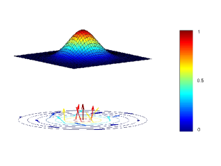
Figure 43: SC vortex with AF core. Far from the center of the vortex core, the superspin vector lies in the SC plane and winds around the vortex core by $2\pi$. The superspin vector lifts up to the AF direction as it approaches the center of the vortex core. The arrows represent the direction of the superspin and the color scale represents the magnitude of the AF order parameter.

A fundamental prediction of the $SO(5)$ theory is the smooth rotation from the AF state to the SC state as the doping density is varied. As shown in sections V.2 and V.3, this prediction has been tested numerically within the $t-J$ model, with good agreement. However, testing this prediction directly in experiments would be much harder, since the doping level of most cuprates cannot be controlled well in the regime where the transition from the AF to SC state is expected to occur. Therefore, ZhangZhang (1997) and Arovas et alArovas et al. (1997) proposed testing this prediction in the vortex state of underdoped cuprates. Around the center of the vortex core, the phase of the SC order parameter winds by $\pm 2\pi$, and the amplitude of the SC order parameter is constrained to vanish at the center for topological reasons. In conventional BCS superconductors, the metallic Fermi liquid ground state is realized inside the vortex core. In the $SO(5)$ theory, the SC order parameter is embedded as components of a higher dimensional order parameter, namely the superspin. When the amplitude of the SC order parameter vanishes in the vortex core, the amplitude of the superspin order parameter can still remain constant, provided that the superspin vector slowly rotates from the SC direction into the AF direction as the vortex core is approached. The superspin configuration near the vortex core is shown in Fig. 43. This type of topological field configuration is known as the meron solution, meaning half of a SkyrmionRajaraman (1982). Fig. 43 shows the rotation of the superspin in the vicinity of a vortex core. The AF order, which develops around the center of the vortex core, can be measured directly in experiments and can provide a quantitative test of the $SO(5)$ symmetry.

The key idea behind this prediction is more general. When the SC order is destroyed in the vortex core, the closest competing order develops in the vortex state. Aside from the commensurate or incommensurate magnetic and charge order, a number of novel correlation states have been proposed, including, for example, the circulating orbital currentsChakravarty et al. (2001); Lee (2002) and the fractionalized excitationsSachdev (1992); Senthil and Fisher (2001). Therefore, the vortex core state can provide a key test for various forms of the competing orders that have been proposedSachdev and Zhang (2002).

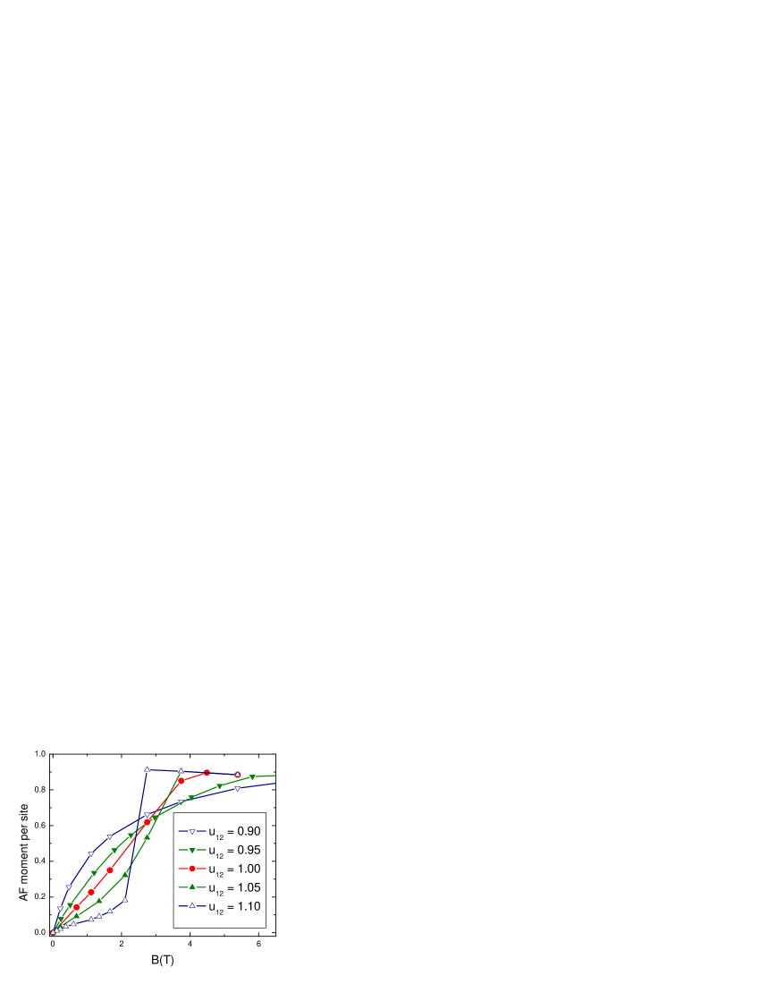
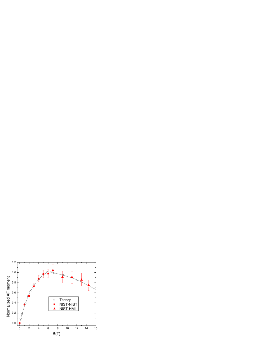
(a)	(b)

Figure 44: The plot of field dependence of the AF moment for different parameters of the LG theory (defined in Ref. Chen et al. (2003b)). The parameters are $\rho_{1}=\rho_{2}=a^{2}$, $r_{1}=-1$, $r_{2}=-0.85$, $u_{1}=u_{2}=1$ and $\chi=42.4$. Here the parameters are chosen such that the maximum SC order is $1$ and the SC coherence length at zero field equals the lattice constant $a$ of the lattice model. (a) Field dependence for different values of $u_{12}$. The curvature strongly depends on $u_{12}$. (b) Fit to the neutron scattering resultsKang et al. (2003) of the $Nd_{1.85}Ce_{0.15}CuO_{4}$ crystal with $u_{12}=0.95$. $B_{c2}$ is about $6.2T$ in this sample. The experimental data is obtained by subtracting the magnetic field response along the $c$ axis by the magnetic field response in the $ab$ plane, so that the response from the $Nd$ moment can be removed.

Magnetic field provides a clean tuning parameter that can be used to investigate quantum transitions between the SC and AF phases. By solving both the $SO(5)$ non-linear sigma model and the LG model of competing AF and SC order parameters, Arovas et alArovas et al. (1997) predicted the existence of the AF vortex state in the underdoped cuprates and further suggested a systematic experimental search for the AF vortex state in neutron scattering and muon spin rotation experiments. These authors also predicted that the magnetic field induced AF moment should increase linearly with the applied magnetic field, or the number of vortices in the system, when the applied magnetic field is small compared to the upper critical field $B_{c2}$. While the original analysis of Arovas et al focused on the regime where the transition between AF and SC is a direct first order transition (corresponding to Fig. 10a of the phase diagram), Demler et alDemler et al. (2001); Zhang et al. (2002) analyzed the case in which there are two second order phase transitions with an intervening uniform AF/SC mixed phase, corresponding to Fig. 10c of the phase diagram. In this case the AF order extends far beyond the vortex core region. Analysis in Refs. Demler et al. (2001); Zhang et al. (2002) demonstrated that the suppression of the SC order in this regime is dominated by the circulating super-currents and leads to a logarithmic correction to the linear dependence of the field induced moment. Recently, a number of experiments have been performed to test the prediction of AF order in the vortex state. Neutron scattering under a magnetic field can directly measure the field induced AF moment. Katano et alKatano et al. (2000) measured enhanced magnetic scattering in the $La_{2-x}Sr_{x}CuO_{4}$ crystal at $x=12\%$ doping. The intensity of elastic magnetic peaks around the $(\pi,\pi)$ point increases at $B=10T$ by as much as $50\%$. Lake et alLake et al. (2001) observed enhanced dynamic AF spin fluctuations in optimally doped $La_{2-x}Sr_{x}CuO_{4}$ crystal at $x=16\%$ doping in an applied magnetic field. Without an applied field, the SC state has a spin gap of about $6meV$. An applied field of $B=7T$ introduces a spectral weight in the energy range of $3\sim 4meV$. The mixed AF/SC phase has been also investigated in both the underdoped $La_{2-x}Sr_{x}CuO_{4}$ crystal at $x=10\%$ doping and in the $La_{2}CuO_{4+y}$ crystal. In both materials the applied magnetic field strongly enhances the quasi-static AF orderingLake et al. (2002); Khaykovich et al. (2002). The field dependence of the induced AF scattering is approximately linear, as predicted in Ref. Arovas et al. (1997), and it agrees quantitatively with the $B\log(B/B_{c2})$ form proposed in Ref. Demler et al. (2001), with the correct value of $B_{c2}$. Another method to measure the AF order is the nuclear magnetic resonance (NMR). In the vortex state, the magnetic field is distributed inhomogeneously over the sample, with the maxima centered at the vortex cores. Therefore, the NMR frequency correlates directly with the location of the nucleus in the vortex lattice. Using NMR on the ${}^{17}O$ nucleus of $YBa_{2}Cu_{3}O_{7}$ under a magnetic field as high as $40T$, Mitrovic et alMitrovic et al. (2001, 2003) detected a sharp increase of the $1/T_{1}T$ rate near the vortex core as the temperature is lowered, indicating enhanced AF ordering (see also Ref.Curro et al. (2000)). Kakuyanagi et alKakuyanagi et al. (2002) performed $Tl$ NMR in the $Tl_{2}Ba_{2}CuO_{6+\delta}$ sample. $Tl$ NMR provides a more direct test of the AF ordering, since ${}^{205}Tl$ nucleus is located directly above the $Cu$ spins. The temperature dependence of the $1/T_{1}T$ rate shows that the AF spin correlation is significantly enhanced inside the vortex core, compared with regions outside. The last class of magnetic experiments we discuss is the muon spin rotation ($\mu$sR) experiments. When muons are stopped inside a solid, their spin precesses around the local magnetic field. Since the muon decays predominantly along the direction of its spin, the spatial decay pattern yields direct information about the local magnetic field distribution in a solid. Miller et alMiller et al. (2002) performed a $\mu$sR experiment in the underdoped $YBa_{2}Cu_{3}O_{6.5}$ system under a magnetic field of $B=4T$. They found that the local magnetic field distribution has a staggered pattern, superimposed on a uniform decay away from the vortex core. The staggered magnetic field detected at the muon site is about $18Gauss$. All the experiments discussed above were carried out at fields far below the upper critical field $B_{c2}$, which in hole doped materials typically exceeds $60T$. In order to establish the nature of the competing state, one has to perform experiments close to $B_{c2}$. This was achieved in recent neutron scattering experiments on the electron doped $Nd_{1.85}Ce_{0.15}CuO_{4}$ crystal in magnetic fields up to $14T$, far above the upper critical field, $B_{c2}$ Kang et al. (2003). Kang et al found field induced AF scattering at $(\pi,\pi,0)$ and observed that the AF moment scales approximately linearly with the applied field up to $B_{c2}$. The AF moment decreases with the magnetic field in the range between $B_{c2}$ and $14T$. Their experimental data and the theoretical fit are shown in Fig.44. The experimental findings of Kang et alKang et al. (2003) have been confirmed by Fujita et alFujita et al. (2003) in a related, electron doped material $Pr_{1-x}LaCe_{x}CuO_{4}$. While $Nd_{1.85}Ce_{0.15}CuO_{4}$ material contains the magnetic $Nd$ moment, the $Pr_{1-x}LaCe_{x}CuO_{4}$ material studied by Fujita et al does not contain such magnetic ions, thus confirming that the field induced AF moment cannot be due to any spurious effects associated with the $Nd$ momentsMang et al. (2003). As we shall see below, the wide field range of the neutron data enables quantitative comparisons with theoretical models.

Since the original theoretical prediction of the AF vortex state, tremendous theoretical progress has been made on the subject of AF vortex latticesAlama et al. (1999); Bruus et al. (1999); Ogata (1999); Hu (1999a); Mortensen et al. (2000); Han and Lee (2000); Andersen et al. (2000); Demler et al. (2001); Hu and Zhang (2002); Zhang et al. (2002); Juneau et al. (2002); Franz and Tesanovic (2001); Franz et al. (2002a); Ghosal et al. (2002); Kivelson et al. (2002); Chen et al. (2002); Chen and Ting (2002). Based on the variational solution of the $t-J$ model, OgataOgata (1999) concluded that the vortex core has AF with an ordered moment about $10\%$ of the full moment. This calculation established the microscopic basis of the AF vortex core. The initial AF vortex solutions were based on the static mean field theory. In the weak field regime where the vortex cores are separated far from each other, the enhanced AF order can be viewed either as dynamic fluctuations of the AF order parameter due to the finite size of the vortex core, or as the bulk AF fluctuation pulled below the spin gap and spatially bound near the vortex cores. This dynamic picture was developed in Refs.Bruus et al. (1999); Demler et al. (2001); Hu and Zhang (2002) and could apply to experiments by Lake et al in optimally doped LSCO. Classical Monte Carlo calculations of the $SO(5)$ model also show the existence of the AF vortex latticeHu (1999a). While the original theory of the AF vortex state was developed for the commensurate AF order, it can also be generalized to the case where the AF ordering wave vector deviates from the $(\pi,\pi)$ point, as in the case of the LSCO systemZhang et al. (2002); Hu and Zhang (2002). The AF ordering inside the vortex core has a profound effect on the electronic structures of the vortex, since it opens up an insulating-like energy gap inside the vortex core where the conventional SC gap vanishes. The conventional theory for $d$-wave vortices based on Bogoliubov-de Gennes (BdG) mean-field theory predicts a large and broad peak at the Fermi energy in the local density of states (LDOS), the so-called zero-energy peak (ZEP), and at the vortex coreWang and Macdonald (1995). However, scanning tunneling spectroscopy (STS) spectrum in BSCCO, giving the LDOS around the vortex core directly, shows only a small-double peak structure at energies 7 meVPan et al. (2000). A similar situation was observed in YBCO compoundsMaggioaprile et al. (1995). The suppression of the local density of states due to the AF ordering inside the vortex core could naturally explain this phenomenonOgata (1999); Andersen et al. (2000); Chen and Ting (2002). However, other forms of order, or the smallness of the core size could also offer alternative explanationsTsuchiura et al. (2003).

While the experimental observation of the AF vortex state confirms a major prediction of the $SO(5)$ theory, most of these experiments have not directly tested the symmetry between AF and SC in the strictest sense. In the following, we shall discuss two aspects of the AF vortex state which directly pertain to the $SO(5)$ symmetry. The spatial variation of the AF and SC order parameters around vortex core lead to a region of space where both order parameters coexist. In this region, the $\pi$ order parameter, whose magnitude can be quantitatively predicted by the $SO(5)$ orthogonality relation in Eq. (60), also develops. Ghosal, Kallin and BerlinskyGhosal et al. (2002) have quantitatively verified this relationship from their numerical solution of the $t-J$ model around the vortex core. It would be desirable to find a way to measure the $\pi$ order parameter and test this relation experimentally.

The detailed experimental data now available up to $B_{c2}$ in electron doped cuprates allows for a quantitative test of the $SO(5)$ symmetry. As discussed in section IV.1, within models of competing AF and SC order, a crucial test for the $SO(5)$ symmetry is the relation $u^{2}_{12}=u_{1}u_{2}$ for the quartic term in Eq. (78). Deviation from the $SO(5)$ relation determines the curvature of the ground state energy versus doping plot, which can be used to determine the nature of the transition between the AF and SC states. Recently, Chen, Wu and ZhangChen et al. (2003b) numerically solved the LG model with competing AF and SC order in the vortex state and found that the deviation from the $SO(5)$ relation $u^{2}_{12}=u_{1}u_{2}$ also determines the curvature of the field induced AF moment versus the magnetic field plot for magnetic fields up to $B_{c2}$. The neutron scattering data obtained in the NCCO superconductorsKang et al. (2003) can be fitted by $u^{2}_{12}/u_{1}u_{2}=0.95$, showing that this system only has a $5\%$ deviation from the $SO(5)$ symmetry. When the magnetic field exceeds $B_{c2}$, it causes canting of the spin moments, thereby reducing the AF moment while increasing the ferromagnetic moment. Thus the $SO(5)$ theory quantitatively explains the experimental data in the entire magnetic field range below $14T$. The experimental results of Fujita et alFujita et al. (2003) in the $Pr_{1-x}LaCe_{x}CuO_{4}$ material are quantitatively similar. We note that the mean-field analysis of the GL free energy does not include quantum fluctuations of the AF order (the first term in equation (53)). The latter should be important when the AF moments are strongly localized inside the vortex cores. We expect that proximity effect type coupling between neighboring AF vortices should be sufficient to suppress such fluctuations.

In the above discussions we focused on the AF moments of static votices in the SC state. The $SO(5)$ model has also been extended to study thermally activated phase slips in one-dimensional wires Sheehy and Goldbart (1998). One can also construct a dual effect to the AF vortices: Goldbart and Sheehy proposed AF hedgehogs with SC cores in Ref. Goldbart and Sheehy (1998).

VII.2 The pair density wave state

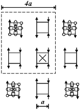
Figure 45: Illustration of the $d$ wave pair density wave state at $x=1/8$. In this state, the $d$ wave hole pairs occupy every four non-overlapping plaquettes on the original lattice. The charge unit cell is $4a\times 4a$. The $SO(5)$ model is defined on the center of the non-overlapping plaquettes. Such a state could be realized around the vortex core, whose center is depicted by the cross. In the actual realization of this state, the hole pair can be much more extended, and the AF ordering could be much reduced from the classical value.

In the quantum disordered phase of the $SO(5)$ model, the hole pair bosons become localized, forming a pair density wave. Since the superfluid density is low and pairing is strong in the underdoped regime of HTSC cuprates, the pair density wave state competes with the $d$ wave SC state. In the global phase diagram shown in Fig. 13, aside from the half-filled AF insulator, there are several possible pair density waver states surrounded by the SC phases. In contrast to the supeconducting state, which can be realized for any charge density, each pair density wave state has a preferred charge density, the dominant one being at doping level $x=1/8$. Since the projected $SO(5)$ model is formulated on the plaquettes of the original lattice, the pair density wave naturally forms a checkerboard pattern, as depicted in Fig. 45. This state has a rotationally symmetric charge periodicity of $4a\times 4a$ near doping level $x=1/8$. However, connecting period of charge modulation to hole density in realistic systems is not always straightforward. In most cases we find states that have both superconductivity and periodic density modulation. Hence, they may be best described as supersolids. Supersolid phases are compressible and can accomodate extra charge without changing the period. Expressed differently, the excess charge can always be taken by the superfluid part of the Cooper pair density without affecting the localized part. The pair density wave state differs from the stripe stateEmery et al. (1999); Zaanen and Gunnarsson (1989), since it does not break the symmetry of $\pi/2$ lattice rotations. It is also distinct from the Wigner crystal of individual holes proposed in Ref.Fu et al. (2004), which should have a charge periodicity of $\sqrt{8}a\times\sqrt{8}a$ at the same doping level. The pair density wave state was first proposed by Chen et alChen et al. (2002) in the context of the $SO(5)$ theory of the vortex state. It also arises naturally from the plaquette boson approach of Altman and AuerbachAltman and Auerbach (2002). Podolsky et al. Podolsky et al. (2003) discussed how unconventional states with translational symmetry breaking, including the pair density wave state, can be detected in STM experiments. Relevance of this state to tunneling experiments has also been considered in Andersen et al. (2003); Vojta (2002); Chen et al. (2004).

As we see in the global phase diagram shown in Fig. 13, the pair density wave state can be stabilized near doping of $x=1/8$, when the superfluid density (or the kinetic energy of the hole pairs) is small compared to interaction energy. This situation can be realized in the vortex core, near the impurities, in the underdoped cuprates or in the pseudo-gap phase. The STM experimentsHoffman et al. (2002) measuring the local density of states near the vortex core demonstrated a $4a\times 4a$ checkerboard pattern, consistent with the hole pair checkerboard stateChen et al. (2002) shown in Fig. 45. The vortex core can be either positively or negatively charged, depending on whether the bulk density is greater or smaller than that of the nearby pair density wave stateWu et al. (2002). For example, if the chemical potential is such that the bulk SC state is on the left (right) side of the $\delta=1/8$ insulator, we expect the vortex core to have more (less) hole density. The STM experiment of Howald et al Howald et al. (2002) sees a similar real space modulation without the applied magnetic field, possibly induced by impuritiesMcElroy et al. (2003) . More recently, Vershinin et al Vershinin et al. (2004) discovered a real space modulation of the density-of-states in the pseudo-gap phase above $T_{c}$. Enhancement of the translational symmetry breaking in the pseudogap regime of the cuprates has been proposed theoretically in Ref. Sachdev and Demler (2003). The microscopic picture of this phenomenon has been studied in Ref. Chen et al. (2004) using an extension of the formalism in Ref. Podolsky et al. (2003) for the pseudogap regime. Analysis of Ref. Chen et al. (2004) shows that the experimentally observed modulation is inconsistent with an ordinary site centered charge density wave and the corresponding modulation of the Hartree-Fock potential. However, the pair density wave state provides good agreement with the experimental data.

VII.3 Uniform mixed phase of antiferromagnetism and superconductivity

The phase diagram obtained from the classical competition between the AF and SC states is shown in Fig. 10. We classified the phase transition broadly into three different types. The “type 1” transition involves a direct first order phase transition between the AF and the SC phases, and the “type 2” transition involves two second order phase transitions, with an intermediate phase which is a uniform mixture of AF and SC. The marginal “type 1.5” transition describes the special $SO(5)$ symmetric case where the chemical potential remains constant in the entire uniform mix phase. Therefore, both “type 2” and “type 1.5” transitions predict a uniform mixed phase of AF and SC.

Evidence for the AF/SC mixed phase exists in the excess oxygen doped $La_{2}CuO_{4+y}$ material. Neutron scattering measurement detects the onset of the AF or spin-density-wave orders at the same temperature as the SC $T_{c}$Lee et al. (1999). This remarkable coincidence is the hallmark of a multi-critical point, which we shall return to later. Because the $La_{2}CuO_{4+y}$ system has an ordering wave vector similar to that of the $La_{2-x}Sr_{x}CuO_{4}$ system, it should also be classified as the “class B3” trace in the global phase diagram of Fig. 13, passing through the “1/8” Mott lobe. However, in this case, the Mott phase boundary likely belongs to “type 1.5 or 2,” where the AF and SC order can coexist.

For $YBa_{2}Cu_{3}O_{6+x}$ materials, static magnetic ordering extending to $x\approx 0.5$ has been observed recently using muon spin rotation/relaxation measurements in Miller et al. (2003). Preliminary neutron scattering experiments in Sidis et al. (2001) and Mook et al. (2002) also reported magnetic ordering with a wavevector $(\pi,\pi)$. Thus, in this case we have AF coexisting with SC without any additional charge order. However, it is unclear if two phases coexist uniformly in these materials. Assuming that future experiments verify the existence of a homogenious phase with AF and SC orders, we conclude that the phase diagram for $YBa_{2}Cu_{3}O_{6+x}$ may be understood as moving along the B1 line line in Figure 13, when the system avoids all the PDW lobes but only has AF and SC orders either separately or in a uniform mixed phase.

Evidence for the mixed phase of superconductivity and antiferromagnetism has also been obtained recently in the five-layered HTSC cuprate $HgBa_{2}Ca_{4}Cu_{5}O_{y}$. In this system, the three inner layers are predominantly antiferromagnetic, while the two outer layers are predominantly superconducting. In a Cu-NMR study, Kotegawa et alKotegawa et al. (2004) obtained firm evidence that the AF inner layers induce a small magnetic moment in the outer layers, establishing the case of an AF/SC uniform mixed phase in this system. However, this type of AF/SC proximity effect was not observed in the artificially grown layer structuresBozovic et al. (2003).

Above discussions show that there is evidence of a uniform mixed phase of AF and SC in the HTSC cuprates. On the other hand, microscopic probes such as STMPan et al. (2001) reveal electronic inhomogeneities characteristic of the “type 1” direct first order transition between AF and SC. Therefore, depending on material details, some HTSC compounds show AF/SC mixed phase, characteristic of the “type 2” behavior, while others show microscopic separation between these two phases, a characteristic more consistent with the “type 1” behavior. It is quite remarkable that such different physical effects can be obtained in materials that are so similar. A reasonable explanation is that the system is actually very close to the $SO(5)$ symmetric point exhibiting “type 1.5” behavior. Only in this case can a slight variation tip the balance towards either the “type 1” or “type 2” behaviors.

A genuine uniform mixed phase of AF and SC has been observed in several heavy-fermion systems in some regions of the pressure (P) versus temperature (T) phase diagram Kitaoka et al. (2001, 2002). Recently, such coexistence was observed through NMR and NQR spectrum measurements in $CeCu_{2}(Si_{1-x}Ge_{x})_{2}$ with a small concentration $x=0.01$ of Ge. In $CeCu_{2}Si_{2}$, SC coexists with slowly fluctuating magnetic waves. However, for AF $CeCu_{2}Ge_{2}$, which has the same lattice and electronic structure as $CeCu_{2}Si_{2}$, it was found that a SC phase can be reached at a critical pressure $P_{c}\sim 7.6GPa$. Since $CeCu_{2}Si_{2}$ behaves at $P=0$ like $CeCu_{2}Ge_{2}$ at $P_{c}$, it is argued that SC in $CeCu_{2}Si_{2}$ occurs close to an AF phase at $P=0$ corresponding to a critical lattice density $D=D_{c}$. This appears to be the reason for the strong AF fluctuations at $P=0$. A small concentration of Ge expands the unit-cell volume reducing $D$ below $D_{c}$ and is thus sufficient to pin the magnetic fluctuations and to produce AF long-range order within the SC phase. Noting that $D=D_{Si}[1(V_{Ge}-V_{Si})x/V_{Ge}]$ for Ge doping and that $D$ increases with pressure, one can draw a combined phase diagram as a function of lattice density $D$ Kitaoka et al. (2002).

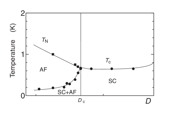
Figure 46: The combined phase diagram as a function of lattice density $D$ in $CeCu_{2}(Si_{1-x}Ge_{x})_{2}$ ($D<D_{c}$ ) and in $CeCu_{2}Si_{2}$ ($D_{c}\leq D$) under pressure $P$. Note that $D\propto 1/V$, where $V$ is the unit-cell volume, and $D=D_{Si}[1(V_{Ge}-V_{Si})x/V_{Ge}]$ in the former case. Reproduced from Ref. Kitaoka et al. (2002).

In Ref. Kitaoka et al. (2002), it was shown that the phase diagram of Fig. 46 could be understood in terms of an $SO(5)$ superspin picture. This could suggest that SC in $CeCu_{2}Si_{2}$ could be mediated by the same magnetic interactions leading to the AF state in $CeCu_{2}(Si_{1-x}Ge_{x})_{2}$.

VII.4 Global phase diagram and multi-critical points

The $SO(5)$ theory makes the key prediction of the existence of a multi-critical point where $T_{N}$ and $T_{c}$ intersect (see Fig. 10) and the general topology of the global phase diagram in the space of quantum parameters (see Fig. 13). The goal of this section is to establish the connection between the theoretical quantum phase diagram proposed in Section IV.2 and the experimental phase diagrams of various families of cuprates. The underlying assumption for making such a connection is that most of material specific properties can be absorbed into parameters of the effective Hamiltonian given in Eq. (69) and in Eq. (84).

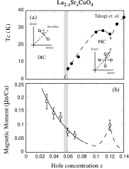
Figure 47: Doping dependence of the SC transition temperature and magnetic moment for $La_{2-x}Sr_{x}CuO_{4}$. Reproduced from Ref. Wakimoto et al. (2001)

One of the most studied phase diagrams of the HTSC is for $La_{2-x}Sr_{x}CuO_{4}$. The stripe order’s presence in these materials has been well documented by neutron scattering experiments Yamada et al. (1998); Wakimoto et al. (2000, 2001). For less than 5% doping the system is in the insulating regime with diagonal stripes and for higher dopings the system is superconducting with collinear stripes (see Fig. 47). It is natural to relate this family of cuprates to the B3 trajectory on the $J/V$-$\mu$ phase diagram shown in Fig. 13: with increasing $\mu$ the system goes through a hierarchy of states at fractional filling factors that correspond to insulating pair density wave states. Near these magic filling factors, the SC $T_{c}$ drops dramatically, while magnetic ordering increases substantially. This is indeed the behavior observed in Fig. 47. As discussed in Section IV.2, the two possible patterns of charge ordering are checkerboard and stripes. In the case of $La_{2-x}Sr_{x}CuO_{4}$, stripe ordering may be stabilized by tilting the $CuO_{6}$ octahedron toward [100] tetragonal direction (parallel to the Cu-O bonds). The phase diagram in Fig. 13 predicts that the ordering wave-vectors take discrete values that correspond to different Mott insulating PDW lobes. For long range interactions PDW phases are very densely packed, so experimentally we may observe an almost continuous dependence of incommensuration on doping, such as the one discussed in Refs. Yamada et al. (1998) and Wakimoto et al. (2000). However, different states in the hierarchy are not equivalent. For example, at $1/8$ doping we have a very strong insulating phase which corresponds to insulating stripes or a simple checkerboard pattern of Cooper pairs (see Fig. 12). This may explain a famous “1/8 anomaly” in the $T_{c}$ vs doping relation for the $La_{2-x}Sr_{x}CuO_{4}$ family of cuprates. Another strong PDW phase is for $1/16$ doping, which may explain why supreconductivity disappears close to this filling (see Fig. 47). A “staircase” of ordering wavevectors for underdoped cuprates has also been discussed in the context of doping the spin-Peierls insulating phase in Refs. Vojta and Sachdev (1999); Sachdev (2002b).

By adding another external parameter we can tune our system continuously between B1 and B3 trajectories. This was done in recent high pressure experiments on $La_{1.48}Nd_{0.4}Sr_{0.12}CuO_{4}$ Locquet et al. (1998); Sato et al. (2000); Arumugam et al. (2002); Takeshita et al. (2003), where the pressure of the order of 0.1 GPa was sufficient to suppress stripe ordering at 1/8 doping and stabilize the high temperature SC phase. Such pressure experiments correspond to moving up along the A2 path in Fig. 13. Applying pressure along this path can directly induce a superconductor to insulator transition.

In contrast to the $LSCO$ family of HTSC cuprates, when one varies the carrier density in the $YBCO$ or $BSCO$ cuprates, there is no evidence for the static charge order. In these materials, charge ordered PDW states can only be realized around vortex coresHoffman et al. (2002), when the effective Cooper pair kinetic energy is reduced, or near impuritiesHowald et al. (2002); McElroy et al. (2003); Vershinin et al. (2004). Therefore, we identify these materials with the B1 trajectories in the global phase diagram of Fig. 13. In this case, the AF/SC boundary can be either be “type 1” or “type 2”. Given the evidence discussed in section VII.3, these systems seem to be close to the “type 1.5” marginal case in between these two types of phase transitions, which means that they should have the approximate $SO(5)$ symmetry.

Within the class of materials exhibiting the “$B1"$ type of trajectory in the global phase diagram, the $SO(5)$ theory makes a distinct prediction of the finite temperature multi-critical point where $T_{c}$ and $T_{N}$ intersect. An interesting issue discussed in Secs. IV.3 and IV is the possibility of analyzing the critical properties of systems (such as many HTSC cuprates) showing a direct transition between an AF and a SC phase. In particular, measuring the critical exponent associated with various physical quantities near the bicritical AF-SC point can give information about the dimension of the symmetry group at the transition Hu and Zhang (2000). Unfortunately, in the HTSC cuprates, sample qualities are not high enough to enable a reliable measurement of the critical behavior near the multi-critical points discussed above. On the other hand, encouraging experimental evidence for an $SO(5)$ bicritical point does exist in a class of 2D organic superconductors called $BEDT$ salt. These material share most common physical properties with the cuprates, and the AF to SC transition can be induced by pressure. In particular, recent experiments on $k-(BEDT-TTF)_{2}X$  Kanoda (1997) revealed an interesting phase diagram in which $T_{c}$ and $T_{N}$ intersect each other at a bicritical point. Kanoda Kanoda (1997) measured the NMR relaxation rate $1/T_{1}$ both in the AF and in the SC region near the bicritical point. Below a characteristic temperature $T^{*}$, $1/T_{1}$ diverges toward the AF transition temperature, while it exhibits a spin-gap-like behavior on the SC side. Murakami and NagaosaMurakami and Nagaosa (2000) analyzed this experimental data in terms of a generalized LG model including both AF and SC fluctuations near the bicritical point. Their study concentrated on the dynamic critical phenomena, in particular the relaxation rate $1/T_{1}$ around the bicritical point. A detailed analysis of the data allowed the extraction of the corresponding critical exponent $x$. Before discussing the NMR line width, we would like to caution the readers that there is also a first order metal-insulator transition in addition to the AF/SC transition discussed hereLefebvre et al. (2000). The presence of the critical endpoint of the metal insulator transition line may lead to some additional complications in the analysis.

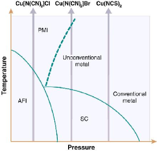
(a)	(b)

Figure 48: (a) Phase diagram the two dimensional organic superconductor BEDT salt. Reproduced from Ref. McKenzie (1997). (b) Log-log plot of $T_{1}^{-1}$ vs $(T-T_{{\rm c}})/T$ for (A) $\kappa$-(BEDT-TTF)₂Cu[N(CN)₂]Cl (solid squares), and (B) deuterated $\kappa$-(BEDT-TTF)₂Cu[N(CN)₂]Br (open squares). (Data from Kawamoto et al. (1995).)

On the AF side of the phase diagram, the NMR line width is proportional to $(T-T_{N})^{-x}$ when approaching $T_{N}$ from the normal state. For systems far away from the bicritical point, the dynamical critical behavior is governed by the $SO(3)$ Heisenberg model, whose exponent $x=x_{3}\approx 0.315$. On the other hand, when the $SO(5)$ bicritical point governs the critical dynamics, the exponent $x$ should change to the $SO(5)$ one $x=x_{5}\approx 0.584$, as obtained from the $\epsilon$-expansion. In Fig. 48, we present a log-log plot of $1/T_{1}$ vs $(T-T_{c})/T$ (from Ref. Murakami and Nagaosa (2000), data from Ref. Kawamoto et al. (1995)) for (A) $\kappa$-(BEDT-TTF)₂Cu[N(CN)₂]Cl (solid squares), and (B) deuterated $\kappa$-(BEDT-TTF)₂Cu[N(CN)₂]Br (open squares). System (A) is located in the AF region away from the bicritical point and system (B) is nearly at the bicritical point. As one can see from the figure, the critical exponent, $x$, is $0.30\pm 0.04$ for system (A) and $0.56\pm 0.04$ for system (B). These values of $x$ are in reasonably good agreement with the theoretical ones, and, in particular, support the fact that the AF/SC bicritical point is governed by the $SO(5)$ symmetric fixed point. This is the first experiment which directly measures the dimension of the symmetry group close to the AF/SC bicritical point and determines $n$ to be close to $5$. More extensive study near the critical region is certainly desired.

A central issue of the HTSC cuprates concerns the phase boundary between the AF and SC phases. It is also in this region that the $SO(5)$ theory makes the most direct and distinct predictions. Current experiments discussed above seem consistent with the zero temperature and finite temperature phase diagrams presented in Fig. 13 and Fig. 10. However, detailed quantitative comparison is still lacking. As the material properties of the HTSC cuprates improve, direct quantitative tests of the $SO(5)$ theory, such as those performed in the organic superconductors, may become possible.

VII.5 The particle-particle resonance mode in the normal state

In this paper we discussed the scenario in which the resonance peak in the inelastic neutron scattering experiments Rossat-Mignod et al. (1991b); Mook et al. (1993); Fong et al. (1995, 1999); He et al. (2001) originates from the triplet $\pi$ mode in the particle-particle channel. This mode does not disappear above $T_{c}$, but it ceases to contribute to the spin fluctuation spectrum, since the particle-particle and particle-hole channels are decoupled from each other in the normal state. An important question to ask is whether one can couple to the $\pi$-channel directly and establish the existence of the resonance already in the normal state. This cannot be done using conventional electro-magnetic probes, which all couple to the particle-hole channels only, but it is possible using tunnelling experiments. Before we discuss the specific proposal of Bazaliy et.al.Bazaliy et al. (1997) for detecting the $\pi$ excitations, it is useful to remind the readers about earlier work on measuring pairing fluctuations in conventional superconductors above their transition temperature Anderson and Goldman (1970). As originally proposed by Scalapino Scalapino (1970), the latter can be measured in a sandwich system of two superconductor SC₁ and SC₂ with different transition temperatures in the regime $T_{c2}<T<T_{c1}$. Resonant coupling between Cooper pairs from the superconductor SC₁ and the fluctuating pairing amplitude in SC₂ leads to the peaks in the IV characteristics at voltages that correspond to half the energy of the “preformed” Cooper pairs in SC₂. The generalization of these tunnelling experiments for detecting the $\pi$ mode in the normal state of the cuprate has been suggested in Bazaliy et al. (1997) and is shown in Fig. 49. In place of the SC₂ region we now have some cuprate material that shows a resonance in the SC state, e.g. an underdoped YBCO, (electrode C in Fig 49), and in place of the SC₁ materials we have a different cuprate superconductor (electrode A in Fig 49) with a higher transition temperature than material C. The system should be in the temperature regime $T_{c}^{C}<T<T_{c}^{A}$. The main difference with the set-up suggested in Ref. Scalapino (1970) is the presence of a thin layer of AF insulator between the A and C electrodes. The reason for this modification is straightforward: we need to probe the $\pi$ channel in the C material that corresponds to the particle-particle mode with spin $S=1$ and momentum $\Pi=(\pi,\pi)$, whereas the SC electrode A provides Cooper pairs with $S=0$ and momentum $q=0$. If the two materials are connected as shown in Fig. 49, a Cooper pair travelling across an AF layer B can emit a magnon, which converts this Cooper pair into a $\pi$-pair and allows resonant coupling between superconductor A and the $\pi$-channel of the “normal” electrode C. One expects to find a resonance in the IV characteristics of the junction with a peak in the tunnelling current at a voltage which is exactly half the energy of the $\pi$-resonance in the C electrode (note that this peak only appears when electrons are injected from A to C, so it appears on one side of the IV curve). A simple qualitative picture described above can be made more precise by considering a tunnelling Hamiltonian between materials A and C

$$H_{T}=\sum_{pk\sigma}T^{d}_{pk}a^{\dagger}_{p\sigma}c_{k\sigma}e^{iVt}+T^{f}_{pk}a^{\dagger}_{p+Q\sigma}c_{k-\sigma}e^{iVt}+h.c.$$ (139)

Here $V$ is the applied voltage, the $a_{p\alpha}$ and $c_{k\alpha}$ operators refer to the electronic operators in A and C with momenta $p$ and $k$. The ratio of the spin flip matrix element $T^{f}_{pk}$ to the direct matrix element $T^{d}_{pk}$ is on the order of $\Delta_{SDW}/U$, where $\Delta_{SDW}$ is the spin-density-wave gap of the AF insulating material B. The diagram responsible for the resonant contribution to the tunnelling current is shown in Fig. 50. The triplet vertex $\Gamma$ takes into account interactions needed to create a sharp $\pi$-resonance in the A electrode. The magnitude of the peak in the tunnelling current was estimated in Ref. Bazaliy et al. (1997) to be 10 $\mu$A$\mu$V for a system of area $10^{-4}$ cm². As argued in section VI, it is not easy to distinguish the particle-hole and the particle-particle origin of the $\pi$ resonance below $T_{c}$ since these two channels are mixed. Direct experimental detection of the triplet particle-particle mode in the normal state would give unambiguous evidence of the particle-particle nature of the $\pi$ resonance mode.

VII.6 Josephson effect in the SC/AF/SC junction

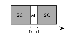
Figure 51: The Superconductor-Antiferromagnet-Superconductor (SC/AF/SC) junction

When discussing the relationship between $d$-wave SC and AF in the HTSC cuprates, one often finds signatures of the nearby magnetic phase in experiments performed on the SC materials. An important question to ask is whether the AF insulating phase shows any signatures of the nearby SC state. An intriguing set of experiments that possibly provides such a demonstration is the long range proximity effect observed in insulating samples of $YBa_{2}Cu_{3}O_{6+x}$ based materials coupled in the $a$-$b$ plane directionsBarner et al. (1991); Hashimoto et al. (1992); Suzuki et al. (1994); Decca et al. (2000). The AF/SC proximity effect was also observed by Kotegawa et alKotegawa et al. (2004), however, it seems to be absent in the case of artificially grown $c$-axis coupled layersBozovic et al. (2003). The appearance of the long range proximity effect is very natural from the point of view of the $SO(5)$ theory, in which low energy degrees of freedom correspond to the order parameter rotation between the AF and SC configurations. A theory of the long range proximity effect within the $SO(5)$ non-linear sigma model has been developed in Ref.Demler et al. (1998a). Let us consider the SC/AF/SC junction shown in Fig. 51. If we set $Re\Delta=\cos\theta\cos\phi$, $Im\Delta=\cos\theta\sin\phi$, and $N_{3}=\sin\theta$, then according to our discussion in Section III.2 (see Eqs. (55)-(58)), the junction can be described by the effective Lagrangian density

$${\cal L}(\theta,\phi)=\frac{\rho}{2}\{(\partial_{i}\theta)^{2}+\cos^{2}\theta~{}(\partial_{i}\phi)^{2}\}-g~{}\sin^{2}\theta.$$ (140)

The anisotropy term is given by $g_{A}>0$ inside the A region, so that the AF phase would be established in the bulk. In the SC S regions on both sides of the junction we have $g_{S}<0$, and we should impose boundary conditions $\theta\rightarrow 0$ as $x\rightarrow\pm\infty$. As discussed in Ref.Demler et al. (1998a), a simplified case corresponds to taking a “strong” superconductor limit for which $\theta(x=0,d)=0$. The current phase relation can now be obtained by writing the Euler-Lagrange equations for the functional (140) at a fixed current. The maximal value of $\theta$ reached at $x=d/2$, $\theta_{0}$, is determined by the equation

$$\frac{d}{2\xi_{A}} = \frac{\cos\theta_{0}}{\sqrt{\omega_{s}^{2}+\cos^{2}\theta_{0}}}K(k)$$

$$k^{2} = \frac{\sin^{2}\theta_{0}\cos^{2}\theta_{0}}{\omega_{s}^{2}+\cos^{2}\theta_{0}},$$ (141)

where $K(k)$ is the the complete elliptic integral of the first kind, dimensionless current $\omega_{s}=I\xi_{A}$, with $I$ being the actual current through the junction and the characteristic length

$$\xi_{A}=\sqrt{\rho/2g_{A}}.$$ (142)

On the other hand, the equation for the phase difference across the junction, $\Delta\Phi$, is given by

$$\Delta\Phi=2\omega_{s}\frac{\cos\theta_{0}}{\sqrt{\omega_{s}^{2}+\cos^{2}\theta_{0}}}\Pi_{1}(-\sin^{2}\theta_{0},k).$$ (143)

Here $\Pi_{1}(n,k)$ is a complete elliptic integral of the third kind. Immediately, one can see that equation (143) describes two different kinds of behavior for $d$ larger or smaller than $d_{c0}=\pi\xi_{A}$. When $d>d_{c0}$ we have a conventional proximity effect with $I(\Delta\Phi)=I_{0}(d)sin\Delta\Phi$ and $I_{0}(d)\propto exp(-d/\xi_{A})$. We observe, however, that the SC correlation length, $\xi_{A}$ may be very long if the system is close to the $SO(5)$ symmetric point ($g_{A}\rightarrow 0$ in equation (142)), which corresponds to the long range proximity effect. When $d<d_{c0}$ we get more intriguing behavior in (143), where for small currents the A region is uniformly superconducting, i.e. $\theta_{0}=0$ (proximity to a strong superconductor completely suppresses the AF order inside the A region), but when the current exceeds some critical value, the system goes into a state that has both $d$-wave SC and AF orders, i.e. $0<\theta_{0}<\pi/2$. The resulting nontrival $I(\Delta\Phi)$ are shown in in Fig. 52. We note that the analysis presented above does not take into account the long range part of the Coulomb interaction between electrons. This may become important for systems with sufficiently wide AF layers and lead to suppression of the proximity induced SC order in the AF layer.

Several consequences of the non-sinusoidal behavior of the current-phase relation of the SAS junctions have been explored in Ref. den Hertog et al. (1999), including current-voltage characteristics in the presense of thermal fluctuations, Shapiro steps, and the Fraunhofer pattern. Decca et.al. Decca et al. (2000) used near-field scanning tunnelling microscopy to photo-generate Josephson junctions in underdoped thin films of $YBa_{2}Cu_{3}O_{6+x}$. They have verified a long range proximity effect through insulating layers but observed a conventional Fraunhofer pattern rather than the one predicted in den Hertog et al. (1999). The geometry of their samples, however, is different from the system studied in Demler et al. (1998a); den Hertog et al. (1999): the intermediate AF layer in their case is connected to large AF regions on both sides of the junctions, which suppresses rotation of the superspin into the SC direction.

In a related context, Auerbach and AltmanAuerbach and Altman (2000) applied the project $SO(5)$ theory to predict multiple Andreev resonance peaks in the SC/AF/SC junctions.

VIII CONCLUSIONS

In a large class of materials including the HTSC cuprates, the organic superconductors and the heavy fermion compounds, the AF and SC phases occur in close proximity to each other. The $SO(5)$ theory is developed based on the assumption that these two phases share a common microscopic origin and should be treated on equal footing. The $SO(5)$ theory gives a coherent description of the rich global phase diagram of the HTSC cuprates and its low energy dynamics through a simple symmetry principle and a unified effective model based on a single quantum Hamiltonian. A number of theoretical predictions, including intensity dependence of the neutron resonance mode, the AF vortex state, the pair-density-wave state and the mixed phase of AF and SC have been verified experimentally. The theory also sheds light on the microscopic mechanism of superconductivity and quantitatively correlates the AF exchange energy with the condensation energy of superconductivity. However, the theory is still incomplete in many ways and lacks full quantitative predictive power. While the role of fermions is well understood within the exact $SO(5)$ models, their roles in the projected $SO(5)$ models are still not fully worked out. As a result, the theory has not made many predictions concerning the transport properties of these materials.

Throughout the history of our quest for the basic laws of nature, symmetry principles have always been the faithful guiding light which time and again led us out of darkness. The enigma of HTSC poses an unprecedented challenge in condensed matter physics. Reflecting upon the historical developments of physical theories, it seems worthwhile to carry out the symmetry approach to the HTSC problem to its full logical conclusion. The basic idea of unifying seemingly different phases by a common symmetry principle may also prove to be useful for other strongly correlated systems.

IX NOTATIONS AND CONVENTIONS

IX.1 Index convention

$\tau^{\alpha}$ denote Pauli matrices.

$\alpha,\beta=x,y,z$ denote $SO(3)$ vector spin indices.

$\sigma,\sigma^{\prime}=1,2$ denote $SO(3)$ spinor indices.

$a,b,c=1,2,3,4,5$ denote $SO(5)$ superspin vector indices.

$\mu,\nu=1,2,3,4$ denote $SO(5)$ spinor indices.

$i,j=1,5$ denote $U(1)$ vector indices for superconductivity.

$x,x^{\prime}$ denote site indices.

IX.2 Dirac $\Gamma$ matrices

The general method introduced by Rabello et. alRabello et al. (1998) to construct $SO(5)$ symmetric models uses the five Dirac $\Gamma$ matrices $\Gamma_{a}$ $(a=1,..,5)$ which satisfy the Clifford algebra,

$$\{\Gamma^{a},\Gamma^{b}\}=2\delta^{ab}.$$ (144)

Rabello et. al introduced the following explicit representation which is naturally adapted for discussing the unification of AF and $d$-wave SC order parameters,

$$\Gamma^{1}\!=\!\left(\begin{array}[]{cc}0&-i\tau_{y}\\ i\tau_{y}&0\end{array}\right)\ \ \ \Gamma^{(2,3,4)}\!=\!\left(\begin{array}[]{cc}\vec{\tau}&0\\ 0&{}^{t}\vec{\tau}\end{array}\right)\ \ \ \Gamma^{5}\!=\!\left(\begin{array}[]{cc}0&\tau_{y}\\ \tau_{y}&0\end{array}\right).$$ (151)

Here $\vec{\tau}=(\tau_{x},\tau_{y},\tau_{z})$ are the usual Pauli matrices and ${}^{t}\vec{\tau}$ denotes their transposition. These five $\Gamma_{a}$ matrices form the $5$ dimensional vector irreps of $SO(5)$. Their commutators,

$$\Gamma^{ab}=-\frac{i}{2}\left[\Gamma^{a},\Gamma^{b}\right],$$ (152)

define the $10$ dimensional antisymmetric tensor irreps of $SO(5)$. In the above representation, the $10$ $\Gamma^{ab}$’s are given explicitly by

$$\Gamma^{15} = \left(\begin{array}[]{cc}-1&0\\ 0&1\end{array}\right)$$ (155)

$$\Gamma^{(i+1)(j+1)} = \varepsilon_{ijk}\left(\begin{array}[]{cc}\tau_{k}&0\\ 0&-{}^{t}\tau_{k}\end{array}\right){}\hskip 19.91692pt(i,j=1,2,3)$$ (158)

$$\Gamma^{(2,3,4)1} = \left(\begin{array}[]{cc}0&-\vec{\tau}\tau_{y}\\ -\tau_{y}\vec{\tau}&0\end{array}\right)=\tau_{y}\left(\begin{array}[]{cc}0&{}^{t}\vec{\tau}\\ -\vec{\tau}&0\end{array}\right)$$ (163)

$$\Gamma^{(2,3,4)5} = \left(\begin{array}[]{cc}0&-i\vec{\tau}\tau_{y}\\ i\tau_{y}\vec{\tau}&0\end{array}\right)=i\tau_{y}\left(\begin{array}[]{cc}0&{}^{t}\vec{\tau}\\ \vec{\tau}&0\end{array}\right).$$ (168)

These $\Gamma$ matrices satisfy the following commutation relations:

$$\left[\Gamma^{ab},\Gamma^{c}\right] = 2i(\delta_{ac}\Gamma^{b}-\delta_{bc}\Gamma^{a})$$ (169)

$$\left[\Gamma^{ab},\Gamma^{cd}\right] = 2i(\delta_{ac}\Gamma^{bd}+\delta_{bd}\Gamma^{ac}-\delta_{ad}\Gamma^{bc}-\delta_{bc}\Gamma^{ad}).$$ (170)

An important property of the $SO(5)$ Lie algebra is the pseudo-reality of its spinor representation. This means that there exists a matrix $R$ with the following properties:

$$R^{2}=-1,\ \ \ R^{\dagger}=R^{-1}={}^{t}R=-R,$$ (171)

$$R\,\Gamma^{a}R=-{}^{t}\Gamma^{a},\ \ \ R\,\Gamma^{ab}R={}^{t}\Gamma^{ab}.$$ (172)

The relations $R\,\Gamma^{ab}R^{-1}=-(\Gamma^{ab})^{*}$ indicate that the spinor representation is real, and the antisymmetric nature of the matrix $R$ indicates that it is pseudo-real. The $R$ matrix plays a role similar to that of $\epsilon_{\alpha\beta}$ in $SO(3)$. In our representation, the $R$ matrix takes the form

$$R=\left(\begin{array}[]{cc}0&1\\ -1&0\end{array}\right).$$ (175)

Figure 3: (a) Zero temperature phase diagram of the XXZ Heisenberg model, the hard-core boson model or the negative $U$ Hubbard model. Phase I is the Ising or the CDW phase, Phase II is the XY or the superfluid phase and phase III is the fully polarized or the normal phase. “Class $A$” transition is induced by the anisotropy parameter $g=J/V$, while the “Class $B$” transition is induced by the chemical potential or the magnetic field. (b) Finite temperature phase diagram for the “class $A$” transition in $D=2$. Because of the $SO(3)$ symmetry at $J=V$ point, the transition temperature vanishes according to the Mermin-Wagner theorem. The dashed line denotes the mean field temperature. (c) Finite temperature phase diagram for the “class $B$” transition in $D=3$. $T_{bc}$ denotes the $SO(3)$ symmetric bicritical point.

Figure 8: Spectra of the collective excitations of the projected $SO(5)$ model as a function of density. The region $0<\rho<\rho_{c}$ corresponds to the uniform mixed phase of SC and AF. Region $\rho>\rho_{c}$ corresponds to the SC phase. The left panel shows the spectra of the spin excitations. For $\rho<\rho_{c}$, there are two gapless spin wave modes and one gapped spin amplitude mode. For $\rho>\rho_{c}$, there is a spin triplet $\pi$ resonance mode. The right panel shows the spectra of the gapless charge excitations (in the absence of long range interactions). For $\rho<\rho_{c}$ the charge mode has quadratic dispersion. The dispersion relation changes from $\omega\propto k^{2}$ to $\omega\propto k$ for the $\rho>\rho_{c}$ regime.

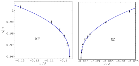
Figure 19: Scaling of $T_{N}$ and $T_{c}$ near the $SO(5)$ bi-critical point. Both $T_{N}$ and $T_{c}$ merge into the bi-critical point tangentially, with the crossover exponent of $\phi=1.43\pm 0.05$.

Figure 23: Eigenstates the spin 3/2 problem on a single site. The longer (shorter) arrows denote —Sz— = 3/2 (1/2) and the up (down) direction denote the +’ (-) sign. The E1,4,6 (singlet), E2,5 (quartet), and E3 (quintet) sets can also be classified as $SO(5)$ singlet, spinor, and vector representations.

Figure 24: Doping dependence of the ground-state energy (two upper curves) and staggered magnetization (lower curve) for the $t-J$ model with $J/t=0.3$. The state with uniform AF and $d$-wave SC order has lower energy compared with the pure $d$-wave SC state for $0<\delta<10\%$, furthermore, the energy of the uniform AF/SC mixed state depends linearly on $\delta$, fitting into the $SO(5)$ symmetric “type 1.5” transition classified in Fig. (9). Reproduced from Ref. Himeda and Ogata (1999).

Figure 25: Exact diagonalization results for the dynamical correlation function of the $\pi$-operator on a 10-site Hubbard system with $U=8t$ reproduced from reference Meixner et al. (1997). A single $\delta$-function-like peak with pronounced weight is visible near $\omega=0$ for the $\pi$-operator, proving the eigenoperator relation (111) in the low-energy regime. This “precession frequency” $\omega_{\pi}$ decreases with decreasing doping. An alternatively constructed “$s$-wave $\pi$-operator”, with $g(p)$ in Eq. (44) given by $g(p)=cosp_{x}+cosp_{y}$, shown in the bottom graph exhibits only incoherent behavior and hardly any weight (note the difference in the $y$-scale). Here $\langle n\rangle$ denotes average electron density, with $\langle n\rangle=1$ being at half-filling.

Figure 32: The order parameter space of the $SO(5)$ theory. $\pi$ operator performs a rotation between the AF and the $d$-wave SC states. This small fluctuation is the new Goldstone mode of the $SO(5)$ theory.

Figure 33: The two particle continuum and the $\pi$ excitation for the tight-biding model. Note, that the continuum of two particle states collapses to a point when the center of mass momentum is $\Pi=(\pi,\pi)$. The $\pi$-mode emerges as an anti-bound state above the continuum.

Figure 34: Dyson’s equation for the $\pi$-resonance. Function $d(p)$ is defined in equation (42).

Figure 35: $\pi$ resonance contribution to the spin susceptibility in the SC state.

Figure 36: Spin susceptibility in the SC state for the model (129) Demler et al. (1998b). The wavevector is along the 0 to $(\pi,\pi)$ direction. Susceptibility was computed using the self-consistent linear response formalism in Fig. 35. The peak at $(\pi,\pi)$ comes from the $\pi$-resonance.

Figure 37: Feynmann diagram for the $\pi$-resonance below $T_{c}$ contrasted with the diagram above $T_{c}$. The cross denotes the anomalous scattering in the SC state which converts a particle into a hole, and vice versa.

Figure 38: Suppression of the resonance intensity by the magnetic field. Reproduced from Ref. Dai et al. (2000).

Figure 39: Doping dependence of the resonance energy and intensity measured in neutron scattering experiments. Reproduced from Ref. Fong et al. (2000).

Figure 40: Temperature dependence of the resonance intensity compared to the specific heat. Reproduced from Ref. Dai et al. (1999).

Figure 41: SC pairing between electrons mediated by exciting a virtual magnon-$\pi$-mode pair.

Figure 42: Diagrammatic representation of the SC pairing mediated by exciting a virtual magnon-$\pi$-mode pair. Solid lines describe electron propogators and dashed lines describe interactions. The upper particle-hole ladder corresponds to the magnon and the lower particle-particle ladder corresponds to the $\pi$-mode.

.

Figure 49: Setting of the tunnelling experiment for detecting the triplet particle-particle $\pi$ mode in the normal state.

Figure 50: Second order tunnelling diagram that gives rise to the resonant coupling of Cooper pairs and $\pi$ excitations in the junction shown in Fig. 49.

Figure 52: Predicted current-phase characteristics of a SC/AF/SC junction with different $d/d_{c0}$.

References

- Abanov et al. (2001) Abanov, A., A. V. Chubukov, and J. Schmalian, 2001, in Journal of Electron Spectroscopy and Related Phenomena 117, 129.
- Abrikosov (2000) Abrikosov, A. A., 2000, in Physica C 341-348, 97.
- Abrikosov et al. (1993) Abrikosov, A. A., L. P. Gorkov, and I. E. Dzyaloshinski, 1993, Methods of quantum field theory in statistical physics (Dover Publications, New York).
- Affleck and Marston (1988) Affleck, I. and J. B. Marston, 1988, in Physical Review B 37(7), 3774.
- Aharony (2002) Aharony, A., 2002, in Physical Review Letters 8805(5), 059703.
- Alama et al. (1999) Alama, S., A. J. Berlinsky, L. Bronsard, and T. Giorgi, 1999, in Physical Review B 60(9), 6901.
- Allen et al. (1999) Allen, S., H. Touchette, S. Moukouri, Y. M. Vilk, and A. M. S. Tremblay, 1999, in Physical Review Letters 83(20), 4128.
- Altman and Auerbach (2002) Altman, E. and A. Auerbach, 2002, in Physical Review B 65(10), 104508.
- Andersen et al. (2000) Andersen, B. M., H. Bruus, and P. Hedegard, 2000, in Physical Review B 61(9), 6298.
- Andersen et al. (2003) Andersen, B. M., P. Hedegard, and H. Bruus, 2003, in Journal of Low Temperature Physics 131(3-4), 281.
- Anderson and Goldman (1970) Anderson, J. T. and A. M. Goldman, 1970, in Physical Review Letters 25(11), 743.
- Anderson (1987) Anderson, P. W., 1987, in Science 235(4793), 1196.
- Anderson (1997) Anderson, P. W., 1997, The Theory of Superconductivity in the High-Tc Cuprate Superconductors (Princeton University Press).
- Anderson et al. (2003) Anderson, P. W., P. A. Lee, M. Randeria, T. M. Rice, N. Trivedi, and F. C. Zhang, 2003, in cond-mat/0311467 .
- Ando et al. (1995) Ando, Y., G. S. Boebinger, A. Passner, T. Kimura, and K. Kishio, 1995, in Physical Review Letters 75(25), 4662.
- Ando et al. (1996) Ando, Y., G. S. Boebinger, A. Passner, N. L. Wang, C. Geibel, and F. Steglich, 1996, in Physical Review Letters 77(10), 2065.
- Arovas et al. (1997) Arovas, D. P., A. J. Berlinsky, C. Kallin, and S. C. Zhang, 1997, in Physical Review Letters 79(15), 2871.
- Arrigoni and Hanke (1999) Arrigoni, E. and W. Hanke, 1999, in Physical Review Letters 82(10), 2115.
- Arrigoni and Hanke (2000) Arrigoni, E. and W. Hanke, 2000, in Physical Review B 62(17), 11770.
- Arumugam et al. (2002) Arumugam, S., N. Mori, N. Takeshita, H. Takashima, T. Noda, H. Eisaki, and S. Uchida, 2002, in Physical Review Letters 88(24), 247001.
- Assaad and Imada (1998) Assaad, F. F. and M. Imada, 1998, in Physical Review B 58(4), 1845.
- Auerbach (1994) Auerbach, A., 1994, Interacting Electrons and Quantum Magnetism (Springer Verlag).
- Auerbach and Altman (2000) Auerbach, A. and E. Altman, 2000, in Physical Review Letters 85(16), 3480.
- Auerbach et al. (2000) Auerbach, A., F. Berruto, and L. Capriotti, 2000, in “Low - dimensional Quantum Field Theories for Condensed Matter Systems - Spin Systems and Strongly Correlated Electrons”. Eds. G. Morandi, P. Sodano, A. Tagliacozzo, V. Tognetti. cond-mat/9801294. .
- Balents et al. (1998) Balents, L., M. P. A. Fisher, and C. Nayak, 1998, in International Journal of Modern Physics B 12(10), 1033.
- Balents et al. (1999) Balents, L., M. P. A. Fisher, and C. Nayak, 1999, in Physical Review B 60(3), 1654.
- Bardasis and Schrieffer (1961) Bardasis, A. and J. R. Schrieffer, 1961, in Physical Review 121(4), 1050.
- Bardeen et al. (1957) Bardeen, J., L. N. Cooper, and J. R. Schrieffer, 1957, in Physical Review 108(5), 1175.
- Barner et al. (1991) Barner, J. B., C. T. Rogers, A. Inam, R. Ramesh, and S. Bersey, 1991, in Applied Physics Letters 59(6), 742.
- Barzykin and Pines (1995) Barzykin, V. and D. Pines, 1995, in Physical Review B 52(18), 13585.
- Baskaran and Anderson (1998) Baskaran, G. and P. W. Anderson, 1998, in Journal of Physics and Chemistry of Solids 59(10-12), 1780.
- Bazaliy et al. (1997) Bazaliy, Y. B., E. Demler, and S. C. Zhang, 1997, in Physical Review Letters 79(10), 1921.
- Bednorz and Müller (1986) Bednorz, J. G. and K. A. Müller, 1986, in Zeitschrift fur Physik B-Condensed Matter 64(2), 189.
- Bernardet et al. (2002) Bernardet, K., G. G. Batrouni, J. L. Meunier, G. Schmid, M. Troyer, and A. Dorneich, 2002, in Physical Review B 65(10), 104519.
- Blumberg et al. (1995) Blumberg, G., B. P. Stojkovic, and M. V. Klein, 1995, in Physical Review B 52(22), 15741.
- Boebinger et al. (1996) Boebinger, G. S., Y. Ando, A. Passner, T. Kimura, M. Okuya, J. Shimoyama, K. Kishio, K. Tamasaku, N. Ichikawa, and S. Uchida, 1996, in Physical Review Letters 77(27), 5417.
- Bouwknegt and Schoutens (1999) Bouwknegt, P. and K. Schoutens, 1999, in Physical Review Letters 82(13), 2757.
- Bozovic et al. (2003) Bozovic, I., G. Logvenov, M. A. J. Verhoeven, P. Caputo, E. Goldobin, and T. H. Geballe, 2003, in Nature 422(6934), 873.
- Brewer et al. (1988) Brewer, J. H., E. J. Ansaldo, J. F. Carolan, A. C. D. Chaklader, W. N. Hardy, D. R. Harshman, M. E. Hayden, M. Ishikawa, N. Kaplan, R. Keitel, J. Kempton, R. F. Kiefl, et al., 1988, in Physical Review Letters 60(11), 1073.
- Brinckmann and Lee (1999) Brinckmann, J. and P. A. Lee, 1999, in Physical Review Letters 82(14), 2915.
- Bruder et al. (1993) Bruder, C., R. Fazio, and G. Schon, 1993, in Physical Review B 47(1), 342.
- Bruus et al. (1999) Bruus, H., K. A. Eriksen, M. Hallundbaek, and P. Hedegard, 1999, in Physical Review B 59(6), 4349.
- Bulut and Scalapino (1996) Bulut, N. and D. J. Scalapino, 1996, in Physical Review B 53(9), 5149.
- Burgess et al. (1998) Burgess, C. P., J. M. Cline, R. MacKenzie, and R. Ray, 1998, in Physical Review B 57(14), 8549.
- Calabrese et al. (2003) Calabrese, P., A. Pelissetto, and E. Vicari, 2003, in Physical Review B 67(5), 054505.
- Calandra and Sorella (2000) Calandra, M. and S. Sorella, 2000, in Physical Review B 61(18), 11894.
- Campuzano et al. (2002) Campuzano, J. C., M. R. Norman, and M. Randeria, 2002, in Physics of Conventional and Unconventional Superconductors, edited by K. H. Bennemann and J. B. Ketterson (Springer-Verlag).
- Capponi and Poilblanc (2002) Capponi, S. and D. Poilblanc, 2002, in Physical Review B 66(18), 180503.
- Carbotte et al. (1999) Carbotte, J. P., E. Schachinger, and D. D. Branch, 1999, in Journal of Low Temperature Physics 117(3-4), 217.
- Carlson et al. (2002) Carlson, E. W., V. J. Emery, S. A. Kivelson, and D. Orgad, 2002, in The Physics of Conventional and Unconventional Superconductors, edited by K. H. Bennemann and J. B. Ketterson (Springer-Verlag).
- Chakravarty et al. (1988) Chakravarty, S., B. I. Halperin, and D. R. Nelson, 1988, in Physical Review Letters 60(11), 1057.
- Chakravarty and Kee (2000) Chakravarty, S. and H. Y. Kee, 2000, in Physical Review B 61(21), 14821.
- Chakravarty et al. (1999) Chakravarty, S., H.-Y. Kee, and E. Abrahams, 1999, in Physical Review Letters 82, 2366.
- Chakravarty et al. (2001) Chakravarty, S., R. B. Laughlin, D. K. Morr, and C. Nayak, 2001, in Physical Review B 6309(9), 094503.
- Chen et al. (2003a) Chen, H.-D., S. Capponi, F. Alet, and S.-C. Zhang, 2003a, in cond-mat/0312660 .
- Chen et al. (2002) Chen, H. D., J. P. Hu, S. Capponi, E. Arrigoni, and S. C. Zhang, 2002, in Physical Review Letters 89(13), 137004.
- Chen et al. (2004) Chen, H.-D., O. Vafek, A. Yazdani, and S.-C. Zhang, 2004, in cond-mat/0402323 .
- Chen et al. (2003b) Chen, H. D., C. J. Wu, and S. C. Zhang, 2003b, in cond-mat/0310289 .
- Chen and Ting (2002) Chen, Y. and C. S. Ting, 2002, in Physical Review B 65(18), 180513.
- Chubukov et al. (2002) Chubukov, A., D. Pines, and J. Schmalian, 2002, in ”The Physics of Conventional and Unconventional Superconductors” edited by K.H. Bennemann and J.B. Ketterson. cond-mat/0201140 .
- Curro et al. (2000) Curro, N. J., C. Milling, J. Haase, and C. P. Slichter, 2000, in Physical Review B 62(5), 3473.
- Dagotto (1994) Dagotto, E., 1994, in Reviews of Modern Physics 66(3), 763.
- Dai et al. (1996) Dai, P., M. Yethiraj, H. A. Mook, T. B. Lindemer, and F. Dogan, 1996, in Physical Review Letters 77(27), 5425.
- Dai et al. (2000) Dai, P. C., H. A. Mook, G. Aeppli, S. M. Hayden, and F. Dogan, 2000, in Nature 406(6799), 965.
- Dai et al. (1998) Dai, P. C., H. A. Mook, and F. Dogan, 1998, in Physical Review Letters 80(8), 1738.
- Dai et al. (1999) Dai, P. C., H. A. Mook, S. M. Hayden, G. Aeppli, T. G. Perring, R. D. Hunt, and F. Dogan, 1999, in Science 284(5418), 1344.
- Damascelli et al. (2003) Damascelli, A., Z. Hussain, and Z. X. Shen, 2003, in Reviews of Modern Physics 75(2), 473.
- Decca et al. (2000) Decca, R. S., H. D. Drew, E. Osquiguil, B. Maiorov, and J. Guimpel, 2000, in Physical Review Letters 85(17), 3708.
- Demler et al. (1998a) Demler, E., A. J. Berlinsky, C. Kallin, G. B. Arnold, and M. R. Beasley, 1998a, in Physical Review Letters 80(13), 2917.
- Demler et al. (1998b) Demler, E., H. Kohno, and S. C. Zhang, 1998b, in Physical Review B 58(9), 5719.
- Demler et al. (2001) Demler, E., S. Sachdev, and Y. Zhang, 2001, in Physical Review Letters 8706(6), 067202.
- Demler and Zhang (1995) Demler, E. and S. C. Zhang, 1995, in Physical Review Letters 75(22), 4126.
- Demler and Zhang (1998) Demler, E. and S. C. Zhang, 1998, in Nature 396(6713), 733.
- Demler and Zhang (1999a) Demler, E. and S. C. Zhang, 1999a, in Annals of Physics 271(1), 83.
- Demler and Zhang (1999b) Demler, E. and S. C. Zhang, 1999b, in Proceedings of the Conference on High Temperature Superconductivity. Eds. S. Barnes, J. Ashkenazi, J. Cohn, and F. Zuo. cond-mat/9903195 .
- Demler et al. (1996) Demler, E., S. C. Zhang, N. Bulut, and D. J. Scalapino, 1996, in International Journal of Modern Physics B 10(17), 2137.
- Doniach and Inui (1990) Doniach, S. and M. Inui, 1990, in Physical Review B 41(10), 6668.
- Dopf et al. (1992) Dopf, G., A. Muramatsu, and W. Hanke, 1992, in Physical Review Letters 68(3), 353.
- Dorneich et al. (2002a) Dorneich, A., W. Hanke, E. Arrigoni, M. Troyer, and S. C. Zhang, 2002a, in Journal of Physics and Chemistry of Solids 63(6-8), 1365.
- Dorneich et al. (2002b) Dorneich, A., W. Hanke, E. Arrigoni, M. Troyer, and S. C. Zhang, 2002b, in Physical Review Letters 88(5), 057003.
- Dorneich and Troyer (2001) Dorneich, A. and M. Troyer, 2001, in Physical Review e 6406(6), 066701.
- Duffy et al. (1998) Duffy, D., S. Haas, and E. Kim, 1998, in Physical Review B 58(10), R5932.
- van Duin and Zaanen (2000) van Duin, C. N. A. and J. Zaanen, 2000, in Physical Review B 61(5), 3676.
- Eder et al. (1999) Eder, R., A. Dorneich, M. G. Zacher, W. Hanke, and S. C. Zhang, 1999, in Physical Review B 59(1), 561.
- Eder et al. (1998) Eder, R., W. Hanke, and S. C. Zhang, 1998, in Physical Review B 57, 13781.
- Emery and Kivelson (1995) Emery, V. J. and S. A. Kivelson, 1995, in Nature 374(6521), 434.
- Emery et al. (1999) Emery, V. J., S. A. Kivelson, and J. M. Tranquada, 1999, in Proceedings of the National Academy of Sciences of the United States of America 96(16), 8814.
- Eschrig and Norman (2000) Eschrig, M. and M. R. Norman, 2000, in Physical Review Letters 85(15), 3261.
- Fisher et al. (1973) Fisher, M. E., M. N. Barber, and D. Jasnow, 1973, in Physical Review A 8(2), 1111.
- Fisher et al. (1989) Fisher, M. P. A., P. B. Weichman, G. Grinstein, and D. S. Fisher, 1989, in Physical Review B 40(1), 546.
- Fong et al. (1999) Fong, H. F., P. Bourges, Y. Sidis, L. P. Regnault, J. Bossy, A. Ivanov, D. L. Milius, I. A. Aksay, and B. Keimer, 1999, in Physical Review Letters 82(9), 1939.
- Fong et al. (2000) Fong, H. F., P. Bourges, Y. Sidis, L. P. Regnault, J. Bossy, A. Ivanov, D. L. Milius, I. A. Aksay, and B. Keimer, 2000, in Physical Review B 61(21), 14773.
- Fong et al. (1995) Fong, H. F., B. Keimer, P. W. Anderson, D. Reznik, F. Dogan, and I. A. Aksay, 1995, in Physical Review Letters 75(2), 316.
- Fong et al. (1996) Fong, H. F., B. Keimer, D. Reznik, D. L. Milius, and I. A. Aksay, 1996, in Physical Review B 54(9), 6708.
- Frahm and Stahlsmeier (2001) Frahm, H. and M. Stahlsmeier, 2001, in Physical Review B 6312(12), 125109.
- Franz et al. (2002a) Franz, M., D. E. Sheehy, and Z. Tesanovic, 2002a, in Physical Review Letters 88(25), 257005.
- Franz and Tesanovic (2001) Franz, M. and Z. Tesanovic, 2001, in Physical Review B 6305(6), 064516.
- Franz et al. (2002b) Franz, M., Z. Tesanovic, and O. Vafek, 2002b, in Physical Review B 66(5), 054535.
- Fu et al. (2004) Fu, H. C., J. C. Davis, and D. H. Lee, 2004, in cond-mat/0403001 .
- Fujimori et al. (1998) Fujimori, A., A. Ino, T. Mizokawa, C. Kim, Z. X. Shen, T. Sasagawa, T. Kimura, K. Kishio, M. Takaba, K. Tamasaku, H. Eisaki, and S. Uchidau, 1998, in Journal of Physics and Chemistry of Solids 59(10-12), 1892.
- Fujita et al. (2003) Fujita, M., M. Matsuda, S. Katano, and K. Yamada, 2003, in cond-mat/0311269 .
- Furusaki and Zhang (1999) Furusaki, A. and S. C. Zhang, 1999, in Physical Review B 60(2), 1175.
- Georgi (1982) Georgi, H., 1982, Lie algebras in particle physics (Addison-Wesley).
- Ghosal et al. (2002) Ghosal, A., C. Kallin, and A. J. Berlinsky, 2002, in Physical Review B 66(21), 214502.
- Goldbart and Sheehy (1998) Goldbart, P. M. and D. E. Sheehy, 1998, in Physical Review B 58(9), 5731.
- Gopalan et al. (1994) Gopalan, S., T. M. Rice, and M. Sigrist, 1994, in Physical Review B 49(13), 8901.
- Greiner (2002) Greiner, M., 2002, in Nature 415, 39.
- Greiter (1997) Greiter, M., 1997, in Physical Review Letters 79(24), 4898.
- Gros (1989) Gros, C., 1989, in Annals of Physics 189(1), 53.
- Halperin et al. (1974) Halperin, B. I., T. C. Lubensky, and S. K. Ma, 1974, in Physical Review Letters 32(6), 292.
- Han and Lee (2000) Han, J. H. and D. H. Lee, 2000, in Physical Review Letters 85(5), 1100.
- Harada and Kawashima (1997) Harada, K. and N. Kawashima, 1997, in Physical Review B 55(18), 11949.
- Harlingen (1995) Harlingen, D. J. V., 1995, in Reviews of Modern Physics 67(2), 515.
- Hashimoto et al. (1992) Hashimoto, T., M. Sagoi, Y. Mizutani, J. Yoshida, and K. Mizushima, 1992, in Applied Physics Letters 60(14), 1756.
- He et al. (2002) He, H., P. Bourges, Y. Sidis, C. Ulrich, L. P. Regnault, S. Pailhes, N. S. Berzigiarova, N. N. Kolesnikov, and B. Keimer, 2002, in Science 295(5557), 1045.
- He et al. (2001) He, H., Y. Sidis, P. Bourges, G. D. Gu, A. Ivanov, N. Koshizuka, B. Liang, C. T. Lin, L. P. Regnault, E. Schoenherr, and B. Keimer, 2001, in Physical Review Letters 86(8), 1610.
- Hebert et al. (2002) Hebert, F., G. G. Batrouni, R. T. Scalettar, G. Schmid, M. Troyer, and A. Dorneich, 2002, in Physical Review B 6501(1), 014513.
- Henley (1998) Henley, C. L., 1998, in Physical Review Letters 80(16), 3590.
- Herbut (2002) Herbut, I. F., 2002, in Physical Review Letters 88(4), 047006.
- den Hertog et al. (1999) den Hertog, B. C., A. J. Berlinsky, and C. Kallin, 1999, in Physical Review B 59(18), R11645.
- Hill et al. (2001) Hill, R. W., C. Proust, L. Taillefer, P. Fournier, and R. L. Greene, 2001, in Nature 414(6865), 711.
- Himeda and Ogata (1999) Himeda, A. and M. Ogata, 1999, in Physical Review B 60(14), R9935.
- Hirsch and Marsiglio (2000) Hirsch, J. E. and F. Marsiglio, 2000, in Physical Review Letters 62, 15131.
- Hirsch et al. (1988) Hirsch, J. E., S. Tang, E. Loh, and D. J. Scalapino, 1988, in Physical Review Letters 60(16), 1668.
- Hoffman et al. (2002) Hoffman, J. E., E. W. Hudson, K. M. Lang, V. Madhavan, H. Eisaki, S. Uchida, and J. C. Davis, 2002, in Science 295(5554), 466.
- Hofstetter et al. (2002) Hofstetter, W., J. I. Cirac, P. Zoller, E. Demler, and M. D. Lukin, 2002, in Physical Review Letters 66, 220407.
- Hong and Salk (1999) Hong, S. P. and S. H. S. Salk, 1999, in Physica B 261, 1053.
- Howald et al. (2002) Howald, C., H. Eisaki, N. Kaneko, M. Greven, and A. Kapitulnik, 2002, in cond-mat/0208442 .
- Howald et al. (2001) Howald, C., R. Fournier, and A. Kapitulnik, 2001, in Physical Review B 6410(10).
- Hu and Zhang (2000) Hu, J.-P. and S.-C. Zhang, 2000, in Physica C 431, 93.
- Hu and Zhang (2001) Hu, J. P. and S. C. Zhang, 2001, in Physical Review B 6410(10), 100502.
- Hu and Zhang (2002) Hu, J. P. and S. C. Zhang, 2002, in Journal of Physics and Chemistry of Solids 63(12), 2277.
- Hu (1999a) Hu, X., 1999a, in cond-mat/9906237 .
- Hu (1999b) Hu, X., 1999b, in Journal of Low Temperature Physics 117(3-4), 289.
- Hu (2001) Hu, X., 2001, in Physical Review Letters 8705(5), 057004.
- Imada et al. (1998) Imada, M., A. Fujimori, and Y. Tokura, 1998, in Reviews of Modern Physics 70(4), 1039.
- Ino et al. (1997) Ino, A., T. Mizokawa, A. Fujimori, K. Tamasaku, H. Eisaki, S. Uchida, T. Kimura, T. Sasagawa, and K. Kishio, 1997, in Physical Review Letters 79(11), 2101.
- Inui et al. (1988) Inui, M., S. Doniach, P. Hirschfeld, and A. E. Ruckenstein, 1988, in Physical Review B 37, 2320.
- Ioffe and Millis (2002) Ioffe, L. B. and A. J. Millis, 2002, in Journal of Physics and Chemistry of Solids 63(12), 2259.
- Jaksch et al. (1998) Jaksch, D., C. Bruder, J. I. Cirac, C. W. Gardiner, and P. Zoller, 1998, in Physical Review Letters 81, 3108.
- Jerome et al. (1980) Jerome, D., A. Mazaud, M. Ribault, and K. Bechgaard, 1980, in Journal de Physique Lettres 41, L95.
- Johnson et al. (2001) Johnson, P. D., T. Valla, A. V. Fedorov, Z. Yusof, B. O. Wells, Q. Li, A. R. Moodenbaugh, G. D. Gu, N. Koshizuka, C. Kendziora, S. Jian, and D. G. Hinks, 2001, in Physical Review Letters 8717(17).
- Jöstingmeier et al. (2003) Jöstingmeier, M., A. Dorneich, E. Arrigoni, W. Hanke, and S.-C. Zhang, 2003, in Physical Review B 68, 245111.
- Juneau et al. (2002) Juneau, M., R. MacKenzie, M. A. Vachon, and J. M. Cline, 2002, in Physical Review B 65(14), 140512.
- Kakuyanagi et al. (2002) Kakuyanagi, K., K. Kumagai, and Y. Matsuda, 2002, in Journal of Physics and Chemistry of Solids 63(12), 2305.
- Kakuyanagi et al. (2003) Kakuyanagi, K., K. Kumagai, Y. Matsuda, and M. Hasegawa, 2003, in Physical Review Letters 90(19).
- Kang et al. (2003) Kang, H. J., P. C. Dai, J. W. Lynn, M. Matsuura, J. R. Thompson, S. C. Zhang, D. N. Argyriou, Y. Onose, and Y. Tokura, 2003, in Nature 423(6939), 522.
- Kanoda (1997) Kanoda, K., 1997, in Hyperfine Interactions 104, 235.
- Kastner et al. (1998) Kastner, M. A., R. J. Birgeneau, G. Shirane, and Y. Endoh, 1998, in Reviews of Modern Physics 70(3), 897.
- Katano et al. (2000) Katano, S., M. Sato, K. Yamada, T. Suzuki, and T. Fukase, 2000, in Physical Review B 62(22), 14677.
- Kawamoto et al. (1995) Kawamoto, A., K. Miyagawa, Y. Nakazawa, and K. Kanoda, 1995, in Physical Review B 52(21), 15522.
- Kee et al. (2002) Kee, H. Y., S. A. Kivelson, and G. Aeppli, 2002, in Physical Review Letters 88(25), 257002.
- Keimer (2004) Keimer, B., 2004, in private communications .
- Khaykovich et al. (2002) Khaykovich, B., Y. S. Lee, R. W. Erwin, S. H. Lee, S. Wakimoto, K. J. Thomas, M. A. Kastner, and R. J. Birgeneau, 2002, in Physical Review B 66(1), 014528.
- Kitaoka et al. (2001) Kitaoka, Y., K. Ishida, Y. Kawasaki, O. Trovarelli, C. Geibel, and F. Steglich, 2001, in Journal of Physics-Condensed Matter 13(4), L79.
- Kitaoka et al. (2002) Kitaoka, Y., Y. Kawasaki, T. Mito, S. Kawasaki, G. Q. Zheng, K. Ishida, D. Aoki, Y. Haga, R. Settai, Y. Onuki, C. Geibel, and F. Steglich, 2002, in Journal of Physics and Chemistry of Solids 63(6-8), 1141.
- Kivelson et al. (1992) Kivelson, S., D. H. Lee, and S. C. Zhang, 1992, in Physical Review B 46(4), 2223.
- Kivelson et al. (2001) Kivelson, S. A., G. Aeppli, and V. J. Emery, 2001, in Proceedings of the National Academy of Sciences of the United States of America 98(21), 11903.
- Kivelson et al. (1998) Kivelson, S. A., E. Fradkin, and V. J. Emery, 1998, in Nature 393(6685), 550.
- Kivelson et al. (2002) Kivelson, S. A., D. H. Lee, E. Fradkin, and V. Oganesyan, 2002, in Physical Review B 66(14), 144516.
- Kohn and Luttinger (1965) Kohn, W. and J. M. Luttinger, 1965, in Physical Review Letters 15(12), 524.
- Kopec and Zaleski (2001) Kopec, T. K. and T. A. Zaleski, 2001, in Physical Review Letters 8709(9), 097002.
- Kopec and Zaleski (2003) Kopec, T. K. and T. A. Zaleski, 2003, in Physica C-Superconductivity and Its Applications 387(1-2), 65.
- Kosterlitz et al. (1976) Kosterlitz, J. M., D. R. Nelson, and M. E. Fisher, 1976, in Physical Review B 13(1), 412.
- Kotegawa et al. (2004) Kotegawa, H., Y. Tokunaga, Y. Araki, G. q. Zheng, Y. Kitaoka, K. Tokiwa, K. Ito, T. Watanabe, A. Iyo, Y. Tanaka, and H. Ihara, 2004, in cond-mat/0401416 .
- Lake et al. (2001) Lake, B., G. Aeppli, K. N. Clausen, D. F. McMorrow, K. Lefmann, N. E. Hussey, N. Mangkorntong, M. Nohara, H. Takagi, T. E. Mason, and A. Schroder, 2001, in Science 291(5509), 1759.
- Lake et al. (2002) Lake, B., H. M. Ronnow, N. B. Christensen, G. Aeppli, K. Lefmann, D. F. McMorrow, P. Vorderwisch, P. Smeibidl, N. Mangkorntong, T. Sasagawa, M. Nohara, H. Takagi, et al., 2002, in Nature 415(6869), 299.
- Lanczos (1950) Lanczos, C., 1950, in Journal of Research of the National Bureau of Standards 45(4), 255.
- Lang et al. (2002) Lang, K. M., V. Madhavan, J. E. Hoffman, E. W. Hudson, H. Eisaki, S. Uchida, and J. C. Davis, 2002, in Nature 415(6870), 412.
- Lanzara et al. (2001) Lanzara, A., P. V. Bogdanov, X. J. Zhou, S. A. Kellar, D. L. Feng, E. D. Lu, T. Yoshida, H. Eisaki, A. Fujimori, K. Kishio, J. I. Shimoyama, T. Noda, et al., 2001, in Nature 412(6846), 510.
- Laughlin (2002) Laughlin, R. B., 2002, in cond-mat/0209269 .
- Lee and Kivelson (2003) Lee, D. H. and S. A. Kivelson, 2003, in Physical Review B 67(2), 024506.
- Lee et al. (2003) Lee, I. J., D. S. Chow, W. G. Clark, J. Strouse, M. J. Naughton, P. M. Chaikin, and S. E. Brown, 2003, in Physical Review B 68, 92510.
- Lee et al. (1997) Lee, I. J., M. J. Naughton, G. Danner, and P. M. Chaikin, 1997, in Physical Review Letters 78, 3555.
- Lee (2002) Lee, P. A., 2002, in Journal of Physics and Chemistry of Solids 63(12), 2149.
- Lee et al. (1999) Lee, Y. S., R. J. Birgeneau, M. A. Kastner, Y. Endoh, S. Wakimoto, K. Yamada, R. W. Erwin, S. H. Lee, and G. Shirane, 1999, in Physical Review B 60(5), 3643.
- Lefebvre et al. (2000) Lefebvre, S., P. Wzietek, S. Brown, C. Bourbonnais, D. Jerome, C. Meziere, M. Fourmigue, and P. Batail, 2000, in Physical Review Letters 85(25), 5420.
- Levi (2002) Levi, B. G., 2002, in Physics Today 55(2), 14.
- Lin et al. (1998) Lin, H. H., L. Balents, and M. P. A. Fisher, 1998, in Physical Review B 58(4), 1794.
- der Linden (1992) der Linden, W. V., 1992, in Physics Reports-Review Section of Physics Letters 220(2-3), 53.
- Liu et al. (1995) Liu, D. Z., Y. Zha, and K. Levin, 1995, in Physical Review Letters 75(22), 4130.
- Locquet et al. (1998) Locquet, J. P., J. Perret, J. Fompeyrine, E. Machler, J. W. Seo, and G. V. Tendeloo, 1998, in Nature 394(6692), 453.
- Loram et al. (1994) Loram, J. W., K. A. Mirza, J. R. Cooper, W. Y. Liang, and J. M. Wade, 1994, in Journal of Superconductivity 7(1), 243.
- Loram et al. (1990) Loram, J. W., K. A. Mirza, and P. F. Freeman, 1990, in Physica C 171(3-4), 243.
- Maggioaprile et al. (1995) Maggioaprile, I., C. Renner, A. Erb, E. Walker, and O. Fischer, 1995, in Physical Review Letters 75(14), 2754.
- Maksimov et al. (1997) Maksimov, E., D. Savrasov, and S. Savrasov, 1997, in Physics-Uspekhi 40, 337.
- Mang et al. (2003) Mang, P., S. Larochelle, and M. Greven, 2003, in cond-mat/0308607 .
- Maple (1998) Maple, M. B., 1998, in Journal of Magnetism and Magnetic Materials 177, 18.
- Markiewicz and Vaughn (1998) Markiewicz, R. S. and M. T. Vaughn, 1998, in Journal of Physics and Chemistry of Solids 59(10-12), 1737.
- Marston et al. (2002) Marston, J. B., J. O. Fjaerestad, and A. Sudbo, 2002, in Physical Review Letters 89(5), 056404.
- Mathur et al. (1998) Mathur, N. D., F. M. Grosche, S. R. Julian, I. R. Walker, D. M. Freye, R. K. W. Haselwimmer, and G. G. Lonzarich, 1998, in Nature 394(6688), 39.
- Mazin and Yakovenko (1995) Mazin, I. I. and V. M. Yakovenko, 1995, in Physical Review Letters 75(22), 4134.
- McElroy et al. (2003) McElroy, K., R. W. Simmonds, J. E. Hoffman, D.-H. Lee, J. Orenstein, H. Eisaki, S. Uchidak, and J. C. Davis, 2003, in Science 422, 592.
- McKenzie (1997) McKenzie, R. H., 1997, in Science 278(5339), 820.
- Meixner et al. (1997) Meixner, S., W. Hanke, E. Demler, and S. C. Zhang, 1997, in Physical Review Letters 79(24), 4902.
- Miller et al. (2003) Miller, R. I., R. F. Kiefl, J. H. Brewer, J. E. Sonier, D. A. Bonn, W. N. Hardy, R. X. Liang, J. M. M nard, and P. Poon, 2003, in preprint .
- Miller et al. (2002) Miller, R. I., R. F. Kiefl, J. H. Brewer, J. E. Sonier, J. Chakhalian, S. Dunsiger, G. D. Morris, A. N. Price, D. A. Bonn, W. H. Hardy, and R. Liang, 2002, in Physical Review Letters 88(13), 137002.
- Millis and Monien (1996) Millis, A. J. and H. Monien, 1996, in Physical Review B 54(22), 16172.
- Mitrovic et al. (2001) Mitrovic, V. F., E. E. Sigmund, M. Eschrig, H. N. Bachman, W. P. Halperin, A. P. Reyes, P. Kuhns, and W. G. Moulton, 2001, in Nature 413(6855), 501.
- Mitrovic et al. (2003) Mitrovic, V. F., E. E. Sigmund, W. P. Halperin, A. P. Reyes, P. Kuhns, and W. G. Moulton, 2003, in cond-mat/0202368 .
- Molegraaf et al. (2002) Molegraaf, H. J. A., Presura, D. van der Marel, P. H. Kes, and M. Li, 2002, in Science 295, 2239.
- Moler et al. (1998) Moler, K. A., J. R. Kirtley, D. G. Hinks, T. W. Li, and M. Xu, 1998, in Science 279, 1193.
- Mook et al. (1998) Mook, H. A., P. C. Dai, S. M. Hayden, G. Aeppli, T. G. Perring, and F. Dogan, 1998, in Nature 395(6702), 580.
- Mook et al. (2002) Mook, H. A., P. C. Dai, S. M. Hayden, A. Hiess, J. W. Lynn, S. H. Lee, and F. Dogan, 2002, in Physical Review B 66(14).
- Mook et al. (1993) Mook, H. A., M. Yethiraj, G. Aeppli, T. E. Mason, and T. Armstrong, 1993, in Physical Review Letters 70(22), 3490.
- Moreo and Scalapino (1991) Moreo, A. and D. J. Scalapino, 1991, in Physical Review Letters 66(7), 946.
- Morningstar and Weinstein (1996) Morningstar, C. J. and M. Weinstein, 1996, in Physical Review D 54(6), 4131.
- Morr and Pines (1998) Morr, D. K. and D. Pines, 1998, in Physical Review Letters 81(5), 1086.
- Mortensen et al. (2000) Mortensen, N. A., H. M. Ronnow, H. Bruus, and P. Hedegard, 2000, in Physical Review B 62(13), 8703.
- Murakami and Nagaosa (2000) Murakami, S. and N. Nagaosa, 2000, in Journal of the Physical Society of Japan 69(8), 2395.
- Murakami et al. (1999) Murakami, S., N. Nagaosa, and M. Sigrist, 1999, in Physical Review Letters 82(14), 2939.
- Nayak (2000) Nayak, C., 2000, in Physical Review B 62(10), R6135.
- Nelson and Kosterlitz (1977) Nelson, D. R. and J. M. Kosterlitz, 1977, in Physical Review Letters 39(19), 1201.
- Norman and Pepin (2003) Norman, M. R. and C. Pepin, 2003, in cond-mat/0302347 .
- Ogata (1999) Ogata, M., 1999, in International Journal of Modern Physics B 13(29-31), 3560.
- Onufrieva and Rossat-Mignod (1995) Onufrieva, F. and J. Rossat-Mignod, 1995, in Physical Review B 52(10), 7572.
- Orenstein (1999) Orenstein, J., 1999, in Nature 401(6751), 333.
- Orenstein and Millis (2000) Orenstein, J. and A. J. Millis, 2000, in Science 288(5465), 468.
- Pan et al. (2000) Pan, S. H., E. W. Hudson, A. K. Gupta, K. W. Ng, H. Eisaki, S. Uchida, and J. C. Davis, 2000, in Physical Review Letters 85(7), 1536.
- Pan et al. (2001) Pan, S. H., J. P. O’Neal, R. L. Badzey, C. Chamon, H. Ding, J. R. Engelbrecht, Z. Wang, H. Eisaki, S. Uchida, A. K. Guptak, K. W. Ng, E. W. Hudson, et al., 2001, in Nature 413(6853), 282.
- Park and Sachdev (2001) Park, K. and S. Sachdev, 2001, in Physical Review B 64, 184510.
- Pich and Frey (1998) Pich, C. and E. Frey, 1998, in Physical Review B 57(21), 13712.
- Pines and Nozieres (1966) Pines, D. and P. Nozieres, 1966, The Theory of Quantum Liquids (Benjamin Cummings).
- Podolsky et al. (2004) Podolsky, D., E. Altman, T. Rostunov, and E. Demler, 2004, in cond-mat/0403406 .
- Podolsky et al. (2003) Podolsky, D., E. Demler, K. Damle, and B. I. Halperin, 2003, in Physical Review B 67(9), 094514.
- Pryadko et al. (2003) Pryadko, L., S. Kivelson, and O. Zachar, 2003, in cond-mat/0306342 .
- Rabello et al. (1998) Rabello, S., H. Kohno, E. Demler, and S. C. Zhang, 1998, in Physical Review Letters 80(16), 3586.
- Rajaraman (1982) Rajaraman, R., 1982, Solitons and Instantons (Elsevier Science).
- Riera (2002a) Riera, J. A., 2002a, in Physical Review B 66(13), 134523.
- Riera (2002b) Riera, J. A., 2002b, in Physical Review B 65(17), 174526.
- Ronning et al. (1998) Ronning, F., C. Kim, D. L. Feng, D. S. Marshall, A. G. Loeser, L. L. Miller, J. N. Eckstein, I. Bozovic, and Z. X. Shen, 1998, in Science 282(5396), 2067.
- Rossat-Mignod et al. (1991a) Rossat-Mignod, J., L. P. Regnault, C. Vettier, P. Bourges, P. Burlet, J. Bossy, J. Y. Henry, and G. Lapertot, 1991a, in Physica C 185, 86.
- Rossat-Mignod et al. (1992) Rossat-Mignod, J., L. P. Regnault, C. Vettier, P. Bourges, P. Burlet, J. Bossy, J. Y. Henry, and G. Lapertot, 1992, in Physica B 180, 383.
- Rossat-Mignod et al. (1991b) Rossat-Mignod, J., L. P. Regnault, C. Vettier, P. Burlet, J. Y. Henry, and G. Lapertot, 1991b, in Physica B 169(1-4), 58.
- Rozhkov and Millis (2002) Rozhkov, A. V. and A. J. Millis, 2002, in Physical Review B 66, 134509.
- Sachdev (1992) Sachdev, S., 1992, in Physical Review B 45(1), 389.
- Sachdev (2000) Sachdev, S., 2000, Quantum Phase Transitions (Cambridge University Press).
- Sachdev (2002a) Sachdev, S., 2002a, in Reviews of Modern Physics 75, 913.
- Sachdev (2002b) Sachdev, S., 2002b, in Annals of Physics 303, 226.
- Sachdev and Bhatt (1990) Sachdev, S. and R. N. Bhatt, 1990, in Physical Review B 41(13), 9323.
- Sachdev and Demler (2003) Sachdev, S. and E. Demler, 2003, in cond-mat/0308024 .
- Sachdev and M.Vojta (2000) Sachdev, S. and M.Vojta, 2000, in Lectures at the NATO Advanced Study Institute/EC Summer School on New Theoretical Approaches to Strongly Correlated Systems. cond-mat/0005250 .
- Sachdev and Zhang (2002) Sachdev, S. and S. C. Zhang, 2002, in Science 295(5554), 452.
- Sandvik (1997) Sandvik, A. W., 1997, in Physical Review B 56(18), 11678.
- Sandvik (1999) Sandvik, A. W., 1999, in Physical Review B 59(22), 14157.
- Sato et al. (2000) Sato, H., A. Tsukada, M. Naito, and A. Matsuda, 2000, in Physical Review B 62(2), R799.
- Scalapino et al. (1998) Scalapino, D., S. C. Zhang, and W. Hanke, 1998, in Physical Review B 58(1), 443.
- Scalapino (1970) Scalapino, D. J., 1970, in Physical Review Letters 24(19), 1052.
- Scalapino (1995) Scalapino, D. J., 1995, in Physics Reports-Review Section of Physics Letters 250(6), 330.
- Scalapino and White (1998) Scalapino, D. J. and S. R. White, 1998, in Physical Review B 58(13), 8222.
- Scalettar et al. (1995) Scalettar, R. T., G. G. Batrouni, A. P. Kampf, and G. T. Zimanyi, 1995, in Physical Review B 51(13), 8467.
- Scalettar et al. (1989) Scalettar, R. T., E. Y. Loh, J. E. Gubernatis, A. Moreo, S. R. White, D. J. Scalapino, R. L. Sugar, and E. Dagotto, 1989, in Physical Review Letters 62(12), 1407.
- Schachinger et al. (2001) Schachinger, E., J. P. Carbotte, and D. N. Basov, 2001, in Europhysics Letters 54(3), 380.
- Schollwoeck et al. (2002) Schollwoeck, U., S. Chakravarty, J. O. Fjaerestad, J. B. Marston, and M. Troyer, 2002, in cond-mat/0209444 .
- Schrieffer (1964) Schrieffer, J. R., 1964, Theory of Superconductivity (Benjamin Cummings).
- Schrieffer et al. (1989) Schrieffer, J. R., X. G. Wen, and S. C. Zhang, 1989, in Physical Review B 39(16), 11663.
- Schulz (1998) Schulz, H., 1998, in cond-mat/9808167 .
- Senthil and Fisher (2001) Senthil, T. and M. P. A. Fisher, 2001, in Physical Review B 6313(13), 134521.
- Senthil et al. (2004) Senthil, T., A. Vishwanath, L. Balents, S. Sachdev, and M. P. A. Fisher, 2004, in Science 303, 1490.
- Sheehy and Goldbart (1998) Sheehy, D. E. and P. M. Goldbart, 1998, in Physical Review B 57(14), R8131.
- Shelton and Senechal (1998) Shelton, D. G. and D. Senechal, 1998, in Physical Review B 58(11), 6818.
- Shen and et al (2004) Shen, K. M. and et al, 2004, in Physical Review B 69, 054503.
- Shen et al. (2002) Shen, Z. X., A. Lanzara, S. Ishihara, and N. Nagaosa, 2002, in Philosophical Magazine B 82, 1349.
- Sidis et al. (2001) Sidis, Y., C. Ulrich, P. Bourges, C. Bernhard, C. Niedermayer, L. P. Regnault, N. H. Andersen, and B. Keimer, 2001, in Physical Review Letters 86(18), 4100.
- Singleton and Mielke (2002) Singleton, J. and C. Mielke, 2002, in Contemporary Physics 43(2), 63.
- Sorella et al. (2002) Sorella, S., G. B. Martins, F. Becca, C. Gazza, L. Capriotti, A. Parola, and E. Dagotto, 2002, in Physical Review Letters 88(11), 117002.
- Stock et al. (2003) Stock, C., W. Buyers, R. Liang, D. Peets, Z. Tun, D. Bonn, W. Hardy, and R. Birgeneau, 2003, in cond-mat/0308168 .
- Suzuki et al. (1994) Suzuki, Y., J. M. Triscone, C. B. Eom, M. R. Beasley, and T. H. Geballe, 1994, in Physical Review Letters 73(2), 328.
- Takeshita et al. (2003) Takeshita, N., T. Sasagawa, T. Sugioka, Y. Tokura1, and H. Takagi, 2003, in cond-mat/0305111 .
- Tallon and Loram (2001) Tallon, J. L. and J. W. Loram, 2001, in Physica C-Superconductivity and Its Applications 349(1-2), 53.
- Taniguchi et al. (2003) Taniguchi, H., K. Kanoda, and A. Kawamoto, 2003, in Physical Review B 67(1), 014510.
- Timusk and Statt (1999) Timusk, T. and B. Statt, 1999, in Reports on Progress in Physics 62(1), 61.
- Tinkham (1995) Tinkham, M., 1995, Introduction to Superconductivity (McGraw Hill).
- Tranquada et al. (1995) Tranquada, J. M., B. J. Sternlieb, J. D. Axe, Y. Nakamura, and S. Uchida, 1995, in Nature 375(6532), 561.
- Tsuchiura et al. (2003) Tsuchiura, H., M. Ogata, Y. Tanaka, and S. Kashiwaya, 2003, in Journal of Low Temperature Physics 131(3-4), 209.
- Tsuei and Kirtley (2000) Tsuei, C. C. and J. R. Kirtley, 2000, in Reviews of Modern Physics 72(4), 969.
- Uemura (2002) Uemura, Y., 2002, in Solid State Communications, Special Issue, edited by Y. U. A.J. Millis, S. Uchida.
- Uemura et al. (1989) Uemura, Y. J., G. M. Luke, B. J. Sternlieb, J. H. Brewer, J. F. Carolan, W. N. Hardy, R. Kadono, J. R. Kempton, R. F. Kiefl, S. R. Kreitzman, P. Mulhern, T. M. Riseman, et al., 1989, in Physical Review Letters 62(19), 2317.
- vanOtterlo et al. (1995) vanOtterlo, A., K. H. Wagenblast, R. Baltin, C. Bruder, R. Fazio, and G. Schon, 1995, in Physical Review B 52(22), 16176.
- Varma (1999) Varma, C. M., 1999, in Physical Review Letters 83(17), 3538.
- Vershinin et al. (2004) Vershinin, M., S. Misra, S. Ono, S. Abe, Y. Ando, and A. Yazdani, 2004, in cond-mat/0402320 .
- Vojta (2002) Vojta, M., 2002, in Physical Review B 66(10), 104505.
- Vojta and Sachdev (1999) Vojta, M. and S. Sachdev, 1999, in Physical Review Letters 83(19), 3916.
- Vonsovsky et al. (1982) Vonsovsky, S. V., Y. A. Izyumov, and E. Z. Kurmaev, 1982, Superconductivity of transition metals (Springer-Verlag, New York).
- Vuletic et al. (2002) Vuletic, T., P. Auban-Senzier, C. Pasquier, D. Jerome, M. Heritier, and K. Bechgaard, 2002, in European Physical Journal B 25, 319.
- Wakimoto et al. (2000) Wakimoto, S., R. J. Birgeneau, M. A. Kastner, Y. S. Lee, R. Erwin, P. M. Gehring, S. H. Lee, M. Fujita, K. Yamada, Y. Endoh, K. Hirota, and G. Shirane, 2000, in Physical Review B 61(5), 3699.
- Wakimoto et al. (2001) Wakimoto, S., R. J. Birgeneau, Y. S. Lee, and G. Shirane, 2001, in Physical Review B 6317(17).
- Wang and Macdonald (1995) Wang, Y. and A. H. Macdonald, 1995, in Physical Review B 52(6), R3876.
- Wegner (2000) Wegner, F. J., 2000, in European Physical Journal B 14(1), 11.
- Weinberg (1995) Weinberg, S., 1995, The Quantum Theory of Fields (Cambridge University Press).
- Wen and Lee (1996) Wen, X. G. and P. A. Lee, 1996, in Physical Review Letters 76(3), 503.
- Weng et al. (1998) Weng, Z. Y., D. N. Sheng, and C. S. Ting, 1998, in Physical Review Letters 80(24), 5401.
- White and Scalapino (1998) White, S. R. and D. J. Scalapino, 1998, in Physical Review Letters 80(6), 1272.
- Wu et al. (2002) Wu, C. J., H. D. Chen, J. P. Hu, and S. C. Zhang, 2002, in cond-mat/0211457 .
- Wu et al. (2003a) Wu, C. J., J. P. Hu, and S. C. Zhang, 2003a, in Physical Review Letters 91, 186402.
- Wu et al. (2003b) Wu, L. A., M. Guidry, Y. Sun, and C. L. Wu, 2003b, in Physical Review B 67(1), 014515.
- Wu et al. (1987) Wu, M. K., J. R. Ashburn, C. J. Torng, P. H. Hor, R. L. Meng, L. Gao, Z. J. Huang, Y. Q. Wang, and C. W. Chu, 1987, in Physical Review Letters 58(9), 908.
- Yamada et al. (1998) Yamada, K., C. H. Lee, K. Kurahashi, J. Wada, S. Wakimoto, S. Ueki, H. Kimura, Y. Endoh, S. Hosoya, G. Shirane, R. J. Birgeneau, M. Greven, et al., 1998, in Physical Review B 57(10), 6165.
- Yang (1989) Yang, C. N., 1989, in Physical Review Letters 63(19), 2144.
- Yang and Zhang (1990) Yang, C. N. and S. C. Zhang, 1990, in Modern Physics Letters B 4(6-7), 759.
- Yeh (2002) Yeh, N., 2002, in Bulletin of Associations of Asia Pacific Physical Socienties (AAPPS) 12, 2.
- Yin et al. (1997) Yin, L., S. Chakravarty, and P. W. Anderson, 1997, in Physical Review Letters 78(18), 3559.
- Yokoyama and Ogata (1996) Yokoyama, H. and M. Ogata, 1996, in Journal of the Physical Society of Japan 65(11), 3615.
- Yoshikawa and Moriya (1999) Yoshikawa, H. and T. Moriya, 1999, in Journal of the Physical Society of Japan 68(4), 1340.
- Zaanen (1999a) Zaanen, J., 1999a, in Physica C 317-318, 217.
- Zaanen (1999b) Zaanen, J., 1999b, in Science 286(5438), 251.
- Zaanen and Gunnarsson (1989) Zaanen, J. and O. Gunnarsson, 1989, in Physical Review B 40(10), 7391.
- Zacher et al. (2000) Zacher, M. G., W. Hanke, E. Arrigoni, and S. C. Zhang, 2000, in Physical Review Letters 85(4), 824.
- Zalcski and Kopec (2000) Zalcski, T. A. and T. K. Kopec, 2000, in Physica C 341, 237.
- Zaleski and Kopec (2000) Zaleski, T. A. and T. K. Kopec, 2000, in Physical Review B 62(13), 9059.
- Zasadzinski et al. (2003) Zasadzinski, J. F., L. Coffey, P. Romano, and Z. Yusof, 2003, in Physical Review B 68, 180504.
- Zhang et al. (1988) Zhang, F. C., C. Gros, T. M. Rice, and H. Shiba, 1988, in Superconductor Science and Technology 1(1), 36.
- Zhang and Rice (1988) Zhang, F. C. and T. M. Rice, 1988, in Physical Review B 37(7), 3759.
- Zhang (1990) Zhang, S. C., 1990, in Physical Review Letters 65(1), 120.
- Zhang (1991) Zhang, S. C., 1991, in International Journal of Modern Physics B 5(1-2), 153.
- Zhang (1997) Zhang, S. C., 1997, in Science 275(5303), 1089.
- Zhang (1998) Zhang, S. C., 1998, in cond-mat/9808309 .
- Zhang et al. (1999) Zhang, S. C., J. P. Hu, E. Arrigoni, W. Hanke, and A. Auerbach, 1999, in Physical Review B 60(18), 13070.
- Zhang et al. (2002) Zhang, Y., E. Demler, and S. Sachdev, 2002, in Physical Review B 66(9), 094501.