Decoupling and Depinning II: Flux lattices in disordered layered superconductors

Abstract

Phase transitions of a flux lattice in layered superconductors with magnetic field perpendicular to the layers and in presence of disorder are studied. We find that disorder generates a random Josephson coupling between layers which leads to a Josephson glass (JG) phase at low temperatures; vanishing of the JG order identifies a depinning transition. We also find that disorder and thermal fluctuations lead to layer decoupling where the renormalized Josephson coupling vanishes. Near decoupling an anharmonic regime is found, where usual elasticity and the resulting Bragg glass are not valid. The depinning line crosses the decoupling line at a multicritical point, resulting in four transition lines. The phase diagram is consistent with the unusual data on $Bi_{2}Sr_{2}CaCu_{2}O_{8}$ such as the ”second peak” and depinning transitions. The Josephson plasma frequency is evaluated in the various phases.

I Introduction

The phase diagram of layered superconductors in a magnetic field $B$ perpendicular to the layers is of considerable interest in view of extensive experiments on high temperature superconductors Kes . A first order transition in $YBa_{2}Cu_{3}O_{7}$ (YBCO) and in $Bi_{2}Sr_{2}CaCu_{2}O_{8}$ (BSCCO) has been interpreted as a melting transition of the flux lattice. The data suggests that the first order line terminates at a multicritical point, which for BSCCO Khaykovich1 ; Khaykovich2 is at $B_{0}\approx 300-10^{3}G$ and $T_{0}\approx 40-50K$, while for YBCO Deligiannis it is at $B_{0}\approx 2-10T$ and $T_{0}\approx 60-80K$, depending on disorder and oxygen concentration. The multicritical point also terminates a ”second peak” transition Kes ; Khaykovich1 ; Khaykovich2 ; Deligiannis which is manifested by a sharp increase in magnetization and in critical current. The transition line at $B\approx B_{0}$ and $T<T_{0}$ is weakly $T$ dependent and was found, for BSCCO, to be smoothly connected with the first order line Avraham . Neutron scattering and $\mu$SR data Kes ; Cubitt show that positional correlations of the flux lattice are significantly reduced near these phase boundaries, except however, near the multicritical point where a reentrant behavior is observed Forgan . Data on $Nd_{1.85}Ce_{0.15}CuO_{4-\delta}$ (NCCO) has also shown a second peak transition; here, however, $B_{0}$ decreases with temperature near the superconducting transition at $T_{c}\approx 23K$ with no apparent multicritical point Giller . The second peak phenomena is also pronounced in other layered systems such as $NbSe_{2}$ Higgins ; Marley and in $Pb/Ge$ multilayers Bruynseraede . Recent decoration data Fasano on $NbSe_{2}$ has shown that the topology of the vortex structure is weakly affected by crossing part of the second peak line. Hence the nature of the phase at $B>B_{0}$ is not well established.

The Josephson plasma resonance is a probe of the Josephson coupling Matsuda ; Koshelev and can be used to probe the various phase transitions. Recent data on BSCCO has indeed shown a significant reduction in the resonance frequency at the second peak transition Shibauchi ; Matsuda2 .

In a remarkable experiment Fuchs et al. Fuchs have shown that the phase diagram of BSSCO is much more elaborate. They show that the spatial distribution of an external current exhibits a transition from bulk pinning to surface pinning of vortices with most of the current flowing at the sample edges. This depinning line crosses the multicritical point and its temperature is almost $B$ independent at $B<B_{0}$. The depinning transition correlates with anomalies in vibrating reed experiments Kopelevich and in magnetization Dewhurst . Thus there are four transition lines which emanate from the multicritical point at $B_{0}$, $T_{0}$: The first order line, the second peak line and depinning lines for both $B<B_{0}$ and $B>B_{0}$. The common intersection of these four transition lines was also seen in data of the c axis Josephson critical current Ooi . This critical current decreases significantly above the second peak line (in contrast with the critical current parallel to the layers) and also decreases in the depinned regimes.

The notion of vortex matter in the presence of disorder has emerged as a fundamental problem of elastic manifolds in a random media Blatter . This has motivated an extensive theoretical effort towards understanding the field-temperature ($B-T$) phase diagram in presence of disorder. Impurity disorder does not allow long range translational order of the flux lattice and finite domains are expected LO . At low temperatures and fields the system is a Bragg glass Giamarchi ; Natterman , i.e. the lattice is dislocation free, at long scales the displacement correlations decay as a power law and Bragg peaks are expected. The impurity induced domains are essential for the description of both equilibrium, e.g. thermodynamic phase transitions and non-equilibrium, e.g. critical current phenomena. Melting, e.g., is expected to occur by thermal or disorder induced dislocations, as indeed demonstrated for fields parallel to the layers Carpentier ; Golub . Numerical simulations on related XY models have also shown disorder induced melting Olson1 ; Nonomura ; Olson2 .

The flux lattice can undergo a transition which is unique to layered superconductors, i.e. a decoupling transition Glazman1 ; Daemen . In this transition the Josephson coupling between layers vanishes while the lattice is maintained by the electro-magnetic coupling between layers. A disorder induced decoupling was also proposed as a crossover phenomena Koshelev1 . Decoupling in presence of columnar defects was also studied Morozov , showing enhancement of the coupled phase.

It has been shown that decoupling coalesces with a defect unbinding transition Dodgson ; ledou which has analogs in isotropic systems Frey . The resulting vacancies and interstitials lead to a reduction in the elastic tilt modulus Marchetti , consistent with the decoupling scenario as described below. It is possible then that a decoupling-defect transition accounts for the peak phenomena in all type II superconductors. The analysis below is, however, presented for layered anisotropic systems where quantitative predictions can be made. Vacancies and interstitials are neglected; their role is dicussed in the concluding section of the preceding companion article GH .

In the present work we expand our previous work HG ; H1 and study effects of disorder at temperatures below the melting temperature $T_{m}$ by employing replica symmetry breaking (RSB) methods. The RSB methods are accurate when couplings of the nonlinear terms are weak. E.g. in the pure case they reproduce the RG result at weak Josephson coupling GH ; in the related problem of vacancies and interstitials it was shown that RSB accurately locates a disorder induced transition ledou . In the present problem weak coupling corresponds to weak Josephson coupling and weak disorder. Weak disorder can be stated as a condition on the size of domains $R_{BG}$ being larger than the renormalized penetration length in the $c$ direction. This condition is examined in section IV and the RSB actually detects this by producing a stronger singularity (appendices A-C). Furthermore, RSB as a variational method can identify order parameters and determine the form of the phase diagram. The critical behavior near the transition, however, is not expected to be accurate.

The most interesting finding in this work is that of a glass order parameter which we term as Josephson glass (JG), as it is due to disorder induced on the Josephson coupling. The JG order is expected to lead to stronger pinning, hence the line where JG vanishes is associated with a depinning line. We find that the JG and decoupling lines cross and lead to four distinct phases which meet at one point in the $B-T$ phase diagram, remarkably close to the experimental phase diagram Fuchs ; Ooi . This paper follows a companion one GH where the decoupling transition is studied in the pure system by second order renormalization group (RG).

The full problem addressed here involves the following set of nonlinearities: (i) Josephson coupling which involves both pancake displacements and a nonsingular phase. (ii) A disordered Josephson coupling which leads to the JG order. (iii) A nonlinear coupling of disorder to the displacement pattern, leading to the well studied Bragg glass (BG) Giamarchi ; Natterman . After presenting the model in section II, we study in section III a simplified version of the full problem in which the nonsingular phase is neglected and also the disorder coupling is linearized, corresponding to scales within finite domains. These approximations lead to an unphysical divergence of an integral $I(z)$ where $z$ is the renormalized Josephson coupling, i.e. $z\rightarrow 0$ at decoupling. In section III we assume that $I(z)$ is convergent and behaves as $\sim\ln z$, an assumption that is justified in appendices A, B and C. In appendix A we extend section III to solve the combined BG/JG system, though the nonsingular phase is neglected. In appendix B the BG system including the non-singular phase is solved, but JG is neglected, as relevant to thermal decoupling. In both appendices A and B we find an additional $\ln^{2}z$ term which signals a divergence of disorder effects in a regime close to decoupling. In appendix C we study JG with the nonsingular phase, but disorder is linearized. It is shown that $I(z)$ converges even in this situation, while an additional $1/\sqrt{z}$ term is generated. In section IV we present a dimensional derivation of domain sizes which correctly reproduces the pinning and BG lengths. Near decoupling there is a regime of nonlinear elasticity with an apparent jump of the tilt modulus $c_{44}$ and the critical current. This anharmonic regime coincides with the onset of the $\ln^{2}z$ term in appendices A, B. In section V the Josephson plasma frequency is studied, being an efficient probe for identifying the various phases. In section VI we discuss available data on the second peak and depinning transitions. We propose that decoupling accounts for the main features of the second peak transition while the depinning transitions correspond to the onset of JG order.

II The Model

Consider a flux lattice with an equilibrium position of the $l$-th flux line at vectors ${\bf R}_{l}$ of a regular two-dimensional lattice. The flux line is composed of a sequence of singular points, or ”pancake” vortices, whose positions at the $n$-th layer can fluctuate to ${\bf R}_{l}+{\bf u}_{l}^{n}$. Of particular interest is the transverse part of ${\bf u}_{l}^{n}$ with the Fourier transform $u_{T}({\bf q},k)$, where ${\bf q},k$ are wavevectors parallel and perpendicular to the layers, respectively. The elastic energy due to the electromagnetic coupling has the form

$${\cal H}_{e-m}=\mbox{$\frac{1}{2}$}\sum_{{\bf q},k}(da^{2})^{2}[c_{66}^{0}q^{2}+c_{44}^{0}(k)k_{z}^{2}]|u_{T}({\bf q},k)|^{2}$$ (1)

where the flux line density is $1/a^{2}$, $d$ is the spacing between layers, ${\bf q}$ is within the Brillouin zone [of area $(2\pi/a)^{2}$], $|k|<\pi/d$ and $k_{z}=(2/d)\sin(kd/2)$. The shear and tilt moduli are given (for $a\gg d$) by GK ; Sudbo ; GH2

$$c_{66}^{0} = \tau/(16da^{2})$$

$$c_{44}^{0}(k) = [\tau/(8da^{2}\lambda_{ab}^{2}k_{z}^{2})]\ln(1+a^{2}k_{z}^{2}/4\pi)$$ (2)

where $\tau=\phi_{0}^{2}d/(4\pi^{2}\lambda_{ab}^{2})$ sets the energy scale and $\lambda_{ab}$ is the magnetic penetration length parallel to the layers; $\tau\approx 10^{3}-10^{4}K$ for YBCO or BSCCO parameters Kes . Note the strong dispersion of $c_{44}^{0}(k)$ so that $c_{44}^{0}(k)$ decreases by the large factor $(d/a)^{2}$ when $k$ varies from $k\lesssim 1/a$ to $1/a\lesssim k<\pi/d$.

The Josephson phase between the layers $n$ and $n+1$ at position ${\bf r}$ in both layers involves contributions from a nonsingular component and from singular vortex terms. The singular phase around a pancake vortex at position ${\bf R}_{l}+{\bf u}_{l}^{n}$ is $\alpha({\bf r}-{\bf R}_{l}-{\bf u}_{l}^{n})$ where $\alpha({\bf r})=\arctan(y/x)$ with ${\bf r}=(x,y)$. We assume that all vortices belong to the flux lines, i.e. there are no free vacancies or interstitials.

The Josephson phase involves the interlayer phase difference from the pancake singularities $\alpha({\bf r}-{\bf R}_{l}-{\bf u}_{l}^{n})-\alpha({\bf r}-{\bf R}_{l}-{\bf u}_{l}^{n+1})$, which after expansion in ${\bf u}_{l}^{n}$ becomes (Eq. 19 of the companion article GH )

$$b_{n}(\mbox{${\bf r}$})=2\pi id\int_{BZ}\frac{d^{2}\mbox{${\bf q}$}dk}{(2\pi)^{3}}e^{-i\mbox{${\bf q}$}\cdot\mbox{${\bf r}$}-iknd}(e^{ikd}-1)\frac{u_{T}(\mbox{${\bf q}$},k)}{\mbox{${\bf q}$}}\,.$$ (3)

We consider first a simplified model which neglects the nonsingular part of the Josephson phase. The nonsingular phase is essential for evaluating displacement fluctuations (section IV), however for the purpose of the phase transitions under study it can be neglected (justified by Appendices A,B). We have then an effective Hamiltonian for wavevectors $|q|<Q_{0}$, (Eq. (23) of the companion article GH )

$${\cal H}_{pure}^{(1)}/T=\mbox{$\frac{1}{2}$}\sum_{\mbox{${\bf q}$},k}c(q,k)q^{2}|b(\mbox{${\bf q}$},k)|^{2}-\frac{E_{J}}{T}\sum_{n}\int d^{2}\mbox{${\bf r}$}\cos b_{n}(\mbox{${\bf r}$})$$ (4)

where $E_{J}$ is the interlayer Josephson coupling energy per unit area and

$$c(q,k)=\frac{a^{4}}{(2\pi d)^{2}T}[c_{44}^{0}(k)+\frac{q^{2}}{k_{z}^{2}}c_{66}^{0}]\equiv c(k)+c^{\prime}\frac{q^{2}}{k_{z}^{2}}$$ (5)

The last equality defines $c(k)$ and $c^{\prime}$, i.e.

$$c(k) = \frac{\tau a^{2}}{32\pi^{2}Td^{3}\mbox{${\lambda_{ab}}$}^{2}}\frac{\ln(1+a^{2}k_{z}^{2}/4\pi)}{k_{z}^{2}}$$

$$c^{\prime} = \frac{\tau a^{2}}{64\pi^{2}Td^{3}}\,.$$ (6)

Since ${\bf\nabla}\alpha\sim 1/r$ decays slowly, even if ${\bf u}_{l}^{n}$ are small the contribution of many vortices which move in phase ($q\rightarrow 0$) leads to a divergent response of $b_{n}({\bf r})$, i.e the $1/q$ factor in Eq. (3). This leads to a decoupling transition Daemen ; HG ; GH , which at weak $E_{J}$ is (Eqs. (27, 40) of the companion article GH )

$$T_{d}^{0}=\frac{4a^{4}}{d^{2}}(\int\frac{dk}{c_{44}^{0}(k)})^{-1}\approx\frac{\tau a^{2}\log(a/d)}{4\pi\lambda_{ab}^{2}}\,.$$ (7)

We note that melting and related dislocations have been neglected. An estimate of $T_{m}$ by the Lindemann criterion yields Blatter ; GH2 $T_{m}\approx\tau$, hence our description near $T_{d}^{0}$ is limited to to $a\lesssim\lambda_{ab}$. Melting in the absence of Josephson coupling was in fact studied melting , showing that $T_{m}$ is between $\tau/8$ and the two-dimensional melting temperature of $\approx 0.004\tau$, approaching the latter at high fields $a\ll\lambda_{ab}$. At intermediate fields the present description is then valid at $a\lesssim 0.4\lambda_{ab}$. However, for disorder induced melting we estimate (see the discussion section VI) that for BSCCO parameters the decoupling field is below the melting field if $a\gtrsim 0.14\lambda_{ab}$, consistent with the low temperature second peak field value.

We proceed now to study the disorder term. A second assumption of the simplified version is that of linearized disorder, i.e. small fluctuations $|{\bf u}_{l}^{n}|\ll a$. Consider a short range pinning potential $U_{pin}^{n}({\bf r})$ with the coupling

$${\cal H}_{pin}=\int d^{2}r\sum_{n,l}U_{pin}^{n}({\bf r})p({\bf r}-{\bf R}_{l}-{\bf u}_{l}^{n})$$ (8)

where $p(\mbox{${\bf r}$})$ is a shape function for a vortex of size $\xi_{0}$ and the disorder has short range correlation

$$\langle U_{pin}^{n}(\mbox{${\bf r}$})U_{pin}^{n^{\prime}}(\mbox{${\bf r}$}^{\prime})\rangle=\mbox{$\frac{1}{2}$}{\bar{U}}\delta_{n,n^{\prime}}\delta(\mbox{${\bf r}$}-\mbox{${\bf r}$}^{\prime})$$ (9)

Expanding Eq. (8) to first order in ${\bf u}_{l}^{n}$ and averaging $U_{pin}^{n}({\bf r})$ by the replica method Mezard ; Giamarchi leads to a disorder term in the free energy

$${\cal H}_{dis}^{(1)}/T=\frac{{\bar{U}}{\bar{p}}}{4T^{2}}\sum_{n.l}\sum_{\alpha,\beta}\mbox{${\bf u}$}_{l}^{n,\alpha}\cdot\mbox{${\bf u}$}_{l}^{n,\beta}$$ (10)

where $\alpha,\beta$ are replica indices. The average involves

$$\int\partial_{i}p(\mbox{${\bf r}$})\partial_{j}p(\mbox{${\bf r}$})d^{2}r=\bar{p}\delta_{ij}$$ (11)

with $\bar{p}$ of order 1.

The replicated Hamiltonian of the simplified version, keeping only transverse displacements, is therefore

$${\cal H}^{(1)}/T = \frac{1}{2}\sum_{{\bf q},k;\alpha,\beta}[c(q,k)q^{2}\delta_{\alpha,\beta}-s_{0}\frac{q^{2}}{k_{z}^{2}}]b^{\alpha}({\bf q},k)b^{\beta*}({\bf q},k)$$ (12)

$$-\frac{E_{J}}{T}\sum_{n;\alpha}\int d^{2}r\,\cos b_{n}^{\alpha}({\bf r})-\frac{E_{v}}{T}\sum_{n;\alpha\neq\beta}\int d^{2}r\cos[b_{n}^{\alpha}({\bf r})-b_{n}^{\beta}({\bf r})]$$

where

$$s_{0}=\frac{\bar{U}\bar{p}}{2T^{2}}\frac{a^{2}d}{(2\pi d^{2})^{2}}\,.$$ (13)

It is found useful below to define a dimensionless disorder parameter $s$,

$$s=\frac{8\pi{\bar{U}}{\bar{p}}\lambda_{ab}^{4}}{\tau^{2}a^{2}\ln^{2}(a/d)}\,.$$ (14)

The inter-replica Josephson coupling, i.e. the $E_{v}$ term in Eq. (12), is generated from the $E_{J}$ term in second order renormalization group (RG). It is essential to keep the $E_{v}$ term from the start since it couples different replica indices and leads to distinct physics by RSB, as shown below. Physically, the $E_{v}$ term originates from random displacements of pancake vortices due to intralayer impurities. The pancake vortices are then not one on top of the other, resulting in random segments of Josephson vortices, i.e. vortices parallel to the layers. The latter represents random Josephson phases, whose replica average leads to the $E_{v}$ term in Eq. (12).

We proceed now to present the full model, which extends Eq. (12) to include the nonsingular phase as well as nonlinear disorder. The Josephson phase involves a nonsingular phase $\theta_{n}(\mbox{${\bf r}$})$ in addition to the pancake fluctuations via $b_{n}(\mbox{${\bf r}$})$. The Hamiltonian of the pure system is then (Eq. 21 of the companion article GH )

$${\cal H}_{pure}\{b,\theta\}/T= \mbox{$\frac{1}{2}$}\sum_{q,k}G_{f}^{-1}({\bf q},k)|\theta({\bf q},k)|^{2}+\mbox{$\frac{1}{2}$}\sum_{{\bf q},k}c({\bf q},k)q^{2}|b({\bf q},k)|^{2}$$ (15)

$$-\frac{E_{J}}{T}\sum_{n}\int d^{2}r\,\cos[\theta_{n}({\bf r})+b_{n}({\bf r})]$$

where

$$G_{f}(q,k)=\frac{4\pi d^{3}T}{\tau q^{2}}(\lambda_{ab}^{-2}+k_{z}^{2})\,.$$ (16)

Consider next the general form of the disorder coupling Blatter . Using the relation $\sum_{l}\delta^{2}(\mbox{${\mbox{\boldmath$\rho$}}$}-\mbox{${\bf R}$}_{l})=\sum_{l}e^{i\mbox{${\bf Q}$}_{l}\cdot\mbox{${\mbox{\boldmath$\rho$}}$}}$ where $\mbox{${\bf Q}$}_{l}$ are reciprocal lattice vectors, the disorder coupling (8) becomes

$${\cal H}_{pin}=-\int d^{2}r\sum_{n}U_{pin}^{n}(\mbox{${\bf r}$})\int\frac{d^{2}\rho}{a^{2}}p[r-\mbox{${\mbox{\boldmath$\rho$}}$}-\mbox{${\bf u}$}^{n}(\mbox{${\mbox{\boldmath$\rho$}}$})]\sum_{l}e^{i\mbox{${\bf Q}$}_{l}\cdot\mbox{${\mbox{\boldmath$\rho$}}$}}$$ (17)

For $|\mbox{${\bf Q}$}_{l}|<1/\xi_{0}$ we can replace $p(\mbox{${\bf r}$})$ by $\xi_{0}^{2}\delta^{2}(\mbox{${\bf r}$})$ so that

$${\cal H}_{pin}=-\frac{\xi_{0}^{2}}{a^{2}}\int d^{2}r\sum_{n}U_{pin}^{n}(\mbox{${\bf r}$})[1+{\mbox{\boldmath$\nabla$}}\cdot\mbox{${\bf u}$}^{n}(\mbox{${\bf r}$})]^{-1}\sum_{l}e^{i\mbox{${\bf Q}$}_{l}\cdot(\mbox{${\bf r}$}-\mbox{${\bf u}$}^{n}(\mbox{${\bf r}$}))}$$ (18)

The coupling to long wavelength modes via ${\mbox{\boldmath$\nabla$}}\mbox{${\bf u}$}^{n}(\mbox{${\bf r}$})$ is irrelevant Giamarchi in 3D so that the replica average of ${\cal H}_{pin}$ becomes

$${\cal H}_{dis}/T=\frac{g_{0}}{a^{2}}\sum_{\mbox{${\bf Q}$},\alpha,\beta,n}\int d^{2}r\cos[\mbox{${\bf Q}$}\cdot(\mbox{${\bf u}$}^{n,\alpha}(\mbox{${\bf r}$})-\mbox{${\bf u}$}^{n,\beta}(\mbox{${\bf r}$}))]$$ (19)

with $g_{0}={\bar{U}}\xi_{0}^{4}/T^{2}a^{2}$. To relate this form to the linearized one (10) we expand in $\mbox{${\bf u}$}^{n,\alpha}(\mbox{${\bf r}$})$ and use $\sum_{\mbox{${\bf Q}$}}\mbox{${\bf Q}$}^{2}\approx\frac{a^{2}}{4\pi}\int^{1/\xi_{0}^{2}}Q^{2}dQ^{2}\approx a^{2}/8\pi\xi_{0}^{4}$ so that (10) is obtained if ${\bar{p}}\approx 1/2\pi$. The coupling $g_{0}$ can then be written as

$$g_{0}=\frac{{\bar{U}}\xi_{0}^{4}}{T^{2}a^{2}}=s\frac{\tau^{2}\xi_{0}^{4}\ln^{2}(a/d)}{4T^{2}\mbox{${\lambda_{ab}}$}^{4}}\,.$$ (20)

We are interested here in BG effects on the $q\rightarrow 0$ singularity associated with the decoupling transition, i.e. the long range properties of the BG. The BG domain size is defined by the scale $R$ where the displacement correlation starts to diverge as $\ln r$. It is reasonable to expect that this scale is determined by the shortest ${\bf Q}$, as indeed shown for a system with regular elasticity Giamarchi , i.e. far from decoupling. We consider then the disorder term with just the shortest reciprocal wavevectors $|\mbox{${\bf Q}$}|\approx 2\pi/a$ (e.g. six wavevectors in the hexagonal lattice). The full Hamiltonian is then

$${\cal H}/T= \sum_{\alpha}\frac{1}{T}{\cal H}_{pure}\{b^{\alpha},\theta^{\alpha}\}-\frac{E_{v}}{T}\sum_{n;\alpha\neq\beta}\int d^{2}r\cos[b_{n}^{\alpha}(\mbox{${\bf r}$})-b_{n}^{\beta}(\mbox{${\bf r}$})+\theta_{n}^{\alpha}(\mbox{${\bf r}$})-\theta_{n}^{\beta}(\mbox{${\bf r}$})]$$ (21)

$$-\frac{g_{0}}{a^{2}}\sum_{\alpha\neq\beta,n}\int d^{2}r\cos[\mbox{${\bf Q}$}\cdot(\mbox{${\bf u}$}^{n,\alpha}(\mbox{${\bf r}$})-\mbox{${\bf u}$}^{n,\beta}(\mbox{${\bf r}$}))]\,.$$

We note finally that a similar two-dimensional (2D) model has been studied by RSB and RG methods H3 ; Scheidl . As shown in the next section, finite values of $k$ dominate the phase transitions, so that a certain $k$ averages of the coefficients in Eq. (12) lead to a 2D problem with the same $q$ singularities as in (12). Indeed the RSB solution below has the same structure as the 2D case H3 with a temperature parameter $t=T/T_{d}^{0}$ and a disorder parameter $s$ (Eq. 14). In view of this similarity, it is useful to quote the RG equations of the 2D model H3 in terms of $u=\xi^{2}E_{J}/T$ and $v=\xi^{2}E_{v}/T$,

$$d\,u = [2u(1-t-s)-2\gamma^{\prime}uvt]d\,\ln\xi$$

$$d\,v = [2v(1-2t)+\mbox{$\frac{1}{2}$}\gamma^{\prime}su^{2}-2\gamma^{\prime}tv^{2}]d\,\ln\xi$$

$$d\,t = -2\gamma^{\prime\prime 2}(t+s)t^{2}u^{2}d\,\ln\xi$$

$$d\,(s/t^{2}) = 16\gamma^{\prime\prime 2}tv^{2}d\,\ln\xi$$ (22)

where the initial value of the scale $\xi$ is $a$ and $\gamma^{\prime},\gamma^{\prime\prime}$ are numbers of order 1. We quote these results so that the necessity of the $E_{v}$ term is shown more concretely. Indeed $E_{v}$ is generated by $sE_{J}^{2}$ while at $t<\frac{1}{2}$ it is relevant on its own. Furthermore, the RG results will be used to qualitatively support and supplement the phase diagram, as derived by RSB in the next section.

III Phase Diagram

In this section we consider the simplified version, Eq. (12). This assumes that displacements are within finite domains and Bragg glass effects are neglected; also the nonsingular phase is neglected here. Appendices A and B show that these assumptions are justified for the purpose of our phase diagram. The nonsingular phase is essential for evaluating displacement fluctuations, as studied in Appendix C.

We proceed by using the RSB method Mezard . The RSB method proceeds by employing a variational free energy ${\cal F}_{var}={\cal F}_{0}+<{\cal H}-{\cal H}_{0}>$ with ${\cal F}_{0}$ the free energy corresponding to

$${\cal H}_{0}=\mbox{$\frac{1}{2}$}\sum_{{\bf q},k;\alpha,\beta}G_{\alpha,\beta}^{-1}({\bf q},k)b^{\alpha}({\bf q},k)b^{\beta*}({\bf q},k)$$ (23)

and $G_{\alpha,\beta}({\bf q},k)$ is determined by an extremum condition on $F_{var}$. We define the following averages $\langle...\rangle_{0}$ with respect to $H_{0}$,

$$\langle\cos b_{n}^{\alpha}(\mbox{${\bf r}$})\rangle_{0} = e^{-\mbox{$\frac{1}{2}$}A_{\alpha}}$$

$$A_{\alpha} = \sum_{{\bf q},k}G_{\alpha,\alpha}(q,k)$$ (24)

$$\langle\cos[b_{n}^{\alpha}(\mbox{${\bf r}$})-b_{n}^{\beta}(\mbox{${\bf r}$})\rangle_{0} = e^{-\mbox{$\frac{1}{2}$}B_{\alpha,\beta}}$$

$$B_{\alpha,\beta} = 2\sum_{{\bf q},k}[G_{\alpha,\alpha}({\bf q},k)-G_{\alpha,\beta}({\bf q},k)]$$ (25)

so that

$${\cal F}_{var}/T= \mbox{$\frac{1}{2}$}\sum_{\mbox{${\bf q}$},k}Tr[\ln G(q,k)+(G^{-1}(q,k)-c(q,k)q^{2}{\hat{I}}-s_{0}\frac{q^{2}}{k_{z}^{2}}{\hat{L}})G(q,k)]$$ (26)

$$-\frac{E_{J}}{T}\sum_{\alpha}e^{-\mbox{$\frac{1}{2}$}A_{\alpha}}-\frac{E_{v}}{T}\sum_{\alpha\neq\beta}e^{-\mbox{$\frac{1}{2}$}B_{\alpha,\beta}}$$

where ${\hat{I}}_{\alpha,\beta}=\delta_{\alpha,\beta}$ and ${\hat{L}}_{\alpha,\beta}=1$.

The variational equation $\delta F_{var}/\delta G_{\alpha,\beta}=0$ yields

$$G_{\alpha,\beta}^{-1}(q,k) = [c(q,k)q^{2}+z]\delta_{\alpha,\beta}-s_{0}(q^{2}/k_{z}^{2})-\sigma_{\alpha,\beta}$$ (27)

$$z = \frac{E_{J}}{Td}e^{-\mbox{$\frac{1}{2}$}A_{\alpha}}$$ (28)

$$\sigma_{\alpha,\beta} = \frac{E_{v}}{Td}[e^{-\mbox{$\frac{1}{2}$}B_{\alpha,\beta}}-\delta_{\alpha,\beta}\sum_{\gamma}e^{-\mbox{$\frac{1}{2}$}B_{\alpha,\gamma}}]$$ (29)

where $z$ is a renormalized Josephson coupling. In the replica limit with the number of replicas $n\rightarrow 0$ the RSB Mezard method represents each matrix as a hierarchy of matrices, e.g. $\sigma_{\alpha,\beta}$ is represented by $\sigma(u)$, with $0<u<1$ and a diagonal component $\tilde{\sigma}$. We parameterize therefore $G_{\alpha,\beta}^{-1}$ by $\tilde{a}$ and $a(u)$, where

$$\tilde{a} = c(q,k)q^{2}-s_{0}\frac{q^{2}}{k_{z}^{2}}+z-\tilde{\sigma}$$

$$a(u) = -s_{0}\frac{q^{2}}{k_{z}^{2}}-\sigma(u)\,.$$ (30)

The amount by which the replica symmetry is broken is measured by a glass order parameter

$$\Delta(u)=u\sigma(u)-\int_{0}^{u}\sigma(v)\,dv\,.$$ (31)

The inverse matrix $G_{\alpha,\beta}$ is represented by $\tilde{b}$ and $b(u)$, where Mezard (see also Appendix B of Ref. H3, )

$$\tilde{b} = \frac{1}{\tilde{a}-\langle a\rangle}\left[\frac{-a(0)}{\tilde{a}-\langle a\rangle}+1+\int_{0}^{1}\frac{dv}{v^{2}}\frac{\Delta(v)}{\tilde{a}-\langle a\rangle+\Delta(v)}\right]$$

$$\tilde{b}-b(u) = \frac{1}{u[\tilde{a}-\langle a\rangle+\Delta(u)]}-\int_{u}^{1}\frac{dv}{v^{2}}\frac{1}{\tilde{a}-\langle a\rangle+\Delta(v)}$$ (32)

and

$$\langle a\rangle=\int_{0}^{1}a(v)dv = s_{0}\frac{q^{2}}{k_{z}^{2}}-\langle\sigma\rangle$$

$$\tilde{a}-\langle a\rangle+\Delta(u) = c(q,k)q^{2}+z+\Delta(u)\,.$$ (33)

$B(u)$ can be written, using (25) and the inversion formula (III), as

$$\mbox{$\frac{1}{2}$}B(u)=\frac{g(u)}{u}-\int_{u}^{1}\frac{g(v)}{v^{2}}$$ (34)

where

$$g(u)=\sum_{\mbox{${\bf q}$},k}\frac{1}{c(k)q^{2}+z+\Delta(u)}=\int\frac{dk}{2\pi}\frac{1}{4\pi c(k)}[\ln\frac{\Delta_{c}}{z+\Delta(u)}]+C_{1}\,.$$ (35)

and

$$C_{1}=\int\frac{dk}{8\pi^{2}c(k)}\ln\frac{c(k)}{c(\pi/d)}\,.$$ (36)

Here $c(q,k)$ of Eq. (5) is replaced by $c(k)$ as defined in (5, II) while the $q^{2}$ term in Eq. (5) amounts to redefining the upper cutoff into $q_{u}^{2}=4\ln(a/d)/\lambda_{ab}^{2}$, (considering $k\approx\pi/d$ as the dominant range of the following $k$ integration) and $\Delta_{c}=c(\pi/d)q_{u}^{2}$. In the following a variable $t$ is temperature in units $T_{d}^{0}$ of the pure system (Eq. 7), i.e.

$$t=\frac{T}{T_{d}^{0}}=\int\frac{dk}{16\pi^{2}}\frac{1}{c(k)}\,.$$ (37)

Eq. (35) is then

$$g(u)=2t\ln\frac{\Delta_{c}}{z+\Delta(u)}+C_{1}\,.$$ (38)

To find $\Delta(u)$ we note that Eq. (29) is equivalent to $\sigma(u)=(E_{v}/Td)\exp[-B(u)/2]$. Differentiating this equation and using $\Delta^{\prime}(u)=u\sigma^{\prime}(u)$ we obtain

$$\frac{\Delta^{\prime}(u)}{u}=-\frac{d}{du}[\frac{\Delta^{\prime}(u)}{g^{\prime}(u)}]\,,$$ (39)

which by using (38) can be written as

$$(\frac{1}{u}-\frac{1}{2t})\frac{d\Delta}{du}=0\,.$$ (40)

The solution of this equation is a one step function, i.e. $\Delta(u)$ jumps at $u=2t$ from zero to a constant value $\Delta_{0}$ at $2t<u<1$. The solution is therefore nontrivial if $t<1/2$.

To complete the solution, the function $B(u)$ from (34) is needed

$$\mbox{$\frac{1}{2}$}B(u) = C_{1}+\ln\frac{\Delta_{c}}{z}+(2t-1)\ln\frac{\Delta_{c}}{z+\Delta_{0}}\qquad u<2t$$ (41)

$$= C_{1}+2t\ln\frac{\Delta_{c}}{z+\Delta_{0}}\qquad\qquad\qquad\qquad 2t<u<1$$

which yields for $\sigma(u)$

$$\sigma(u)=\sigma_{0} = \frac{z}{z+\Delta_{0}}\sigma_{1}\qquad\qquad\qquad u<2t$$

$$\sigma_{1} = \frac{E_{v}}{Td}(\frac{z+\Delta_{0}}{\Delta_{c}})^{2t}e^{-C_{1}}\qquad 2t<u<1\,.$$ (42)

Finally, from Eq. (31) we have $z+\Delta_{0}=2t\sigma_{1}$, hence,

$$\frac{z+\Delta_{0}}{\Delta_{c}}=(\frac{2E_{v}}{dT_{d}^{0}\Delta_{c}}e^{-C_{1}})^{\frac{1}{1-2t}}$$ (43)

A consistent weak coupling solution is indeed possible only at $t<\mbox{$\frac{1}{2}$}$.

To find a second equation for $z$ from (28) we need the first inversion formula in (III)

$$\tilde{G}(q,k)=\frac{\frac{s_{0}}{k_{z}^{2}c(k)}+\frac{1}{2t}}{c(k)q^{2}+z}+\frac{\sigma_{0}-\frac{s_{0}z}{k_{z}^{2}c(k)}}{(c(k)q^{2}+z)^{2}}+\frac{1-\frac{1}{2t}}{c(k)q^{2}+z+\Delta_{0}}$$ (44)

and after the ${\bf q}$ summation

$$A_{\alpha}=\sum_{\mbox{${\bf q}$},k}\tilde{G}(q.k)=\int\frac{dk}{8\pi^{2}}[\frac{1}{2tc(k)}\ln\frac{z+\Delta_{0}}{z}+\frac{1}{c(k)}\ln\frac{\Delta_{c}}{z+\Delta_{0}}+\frac{\sigma_{0}}{zc(k)}]+C_{1}+\frac{s_{0}}{8\pi^{2}}[I(z)+zI^{\prime}(z)]\\$$

where

$$I(z)=\int\frac{dq^{2}dk}{k_{z}^{2}c(k)}\frac{1}{c(k)q^{2}+z}$$ (45)

and $I^{\prime}(z)=dI(z)/dz$. For $\Delta_{0}\neq 0$ we have from Eq. (III) $\sigma_{0}=z/2t$ while for $\Delta_{0}=0$ (possible at $t>\mbox{$\frac{1}{2}$}$ as found below) we have $\sigma_{0}\sim z^{2t}\ll z$, hence, with $s$ defined in (14),

$$A_{\alpha} = \ln(2etE_{v}/zd)+(s_{0}/8\pi^{2})[I(z)+zI^{\prime}(z)]\qquad\Delta_{0}\neq 0$$ (46)

$$= C_{1}+2(t+s)\ln\frac{\Delta_{c}}{z}+2s\qquad\qquad\qquad\qquad\Delta_{0}=0\,.$$ (47)

Formally $I(z)$ diverges at $k=0$; this divergence can be traced back to our assumption that the $\cos[{\bf Q}\cdot({\bf u}_{l}^{n,\alpha}-{\bf u}_{l}^{n,\beta})]$ term is expanded into the $s_{0}$ term in Eq. (12). Retaining this cosine leads to domains of correlated ${\bf u}_{l}^{n}$. In Appendix A the joint BG-JG solution is found and is shown to remove the $k\rightarrow 0$ divergence. A combined BG with non-singular phase solution is also shown in Appendix B to remove this divergence. The presence of BG, however, produces a term $\sim\ln^{2}z$ in a regime near decoupling (Eq. 95 in the regime of Eq. 99). This ”anharmonic” regime is studied further in section IV. Excluding this anharmonic regime, the dominant part of $I(z)$ is

$$I_{0}(z)=2\int_{1/a}^{\pi/d}\frac{dk}{k_{z}^{2}c(k)}\int\frac{dq^{2}}{c(k)q^{2}+z}=\frac{\pi d}{4c^{2}(\pi/d)}\ln\frac{\Delta_{c}}{z}$$ (48)

The $I(z)$ term in Eq. (III) can then be written as

$$\frac{s_{0}}{8\pi^{2}}I(z)\approx\frac{s_{0}}{8\pi^{2}}I_{0}(z)=2s\ln\frac{\Delta_{c}}{z}\,.$$ (49)

Therefore, the renormalized Josephson coupling of Eq. (28) is for $\Delta_{0}\neq 0$, using Eq. (46),

$$\frac{z}{\Delta_{c}}=e^{-1}(\frac{E_{J}^{2}}{2TtdE_{v}\Delta_{c}})^{\frac{1}{1-2s}}\,.$$ (50)

Note that $E_{v}$ is generated from $E_{J}$ by RG H3 ; Scheidl , i.e. $E_{v}\sim E_{J}^{2}$ initially; however, $E_{v}$ is RG relevant at $t<\mbox{$\frac{1}{2}$}$ even in 1st order RG (Eq. II), hence we consider $E_{v}$ and $E_{J}$ as comparable so that $E_{J}^{2}/(2TtdE_{v}\Delta_{c})\ll 1$. Hence a consistent weak coupling $z/\Delta_{c}\ll 1$ solution is possible only for $s<\mbox{$\frac{1}{2}$}$. Thus $s=\mbox{$\frac{1}{2}$}$ marks a disorder induced decoupling with $z=0$ at $s>\mbox{$\frac{1}{2}$}$.

Comparing Eqs. (43,50) shows that $\Delta_{0}$ vanishes at $s=t$ (up to $O[\ln(E_{J}/E_{v})/\ln E_{v}]$ term, small for $E_{J}\approx E_{v}\ll d\Delta_{c}T_{d}$). Formally there is a solution with $\Delta_{0}<0$ when $s<t$. However, the average distribution Mezard of $|b({\bf q},k)|^{2}$, which is $\sim\exp[-|b({\bf q},k)|^{2}/G_{\alpha,\alpha}({\bf q},k)]$, is acceptable only if $G_{\alpha,\alpha}({\bf q},k)>0$; this is therefore a thermodynamic stability criterion. Note in particular from Eq. (44)

$$G_{\alpha\alpha}(q=0,k)=\frac{1}{2t}(\frac{2}{z}-\frac{1-2t}{z+\Delta_{0}})\,.$$ (51)

When $s<t$ and $\Delta_{0}<0$ the power dependence in Eq. (43) implies that $z+\Delta_{0}\ll z$ (unless too close to $t=s$, i.e. $s-t\sim 1/|\ln E_{v}|$) and therefore $G_{\alpha\alpha}(q=0,k)<0$. This shows that only $\Delta_{0}>0$ is acceptable.

Thus the regime where both $z$, $\Delta_{0}$ are finite is limited to $s<\mbox{$\frac{1}{2}$}$, $t<s$; we term this regime the coupled Josephson Glass (JG) phase. The ”coupled” notation means that the renormalized Josephson coupling is finite, i.e. $z\neq 0$. The glass parameter vanishes (continuously) at $t=s$ while the Josephson coupling vanishes (with an apparent discontinuity - see section IV ) at $s=\mbox{$\frac{1}{2}$}$ (see Fig. 1). For $s>\mbox{$\frac{1}{2}$}$ and $t<\mbox{$\frac{1}{2}$}$ the solution is $z=0$ while $\Delta_{0}\neq 0$ satisfies Eq. (43), i.e. it is a decoupled JG phase. Recall that the JG order parameter $\Delta_{0}$ is due to $E_{v}$ which is initially generated by $E_{J}$. In fact, the RG of Eq. (II) shows (see a similar effect in Fig. 3 of the companion article GH for the pure system) that $E_{J}$ first increases (scaling from $\xi_{0}$ to $1/q_{u}$), generating the $E_{v}$ term, and only at scales beyond $1/q_{u}$ $E_{J}$ decreases to zero. It is remarkable then that $E_{J}$ is renormalized to zero while the JG order survives, much like the smile of the Cheshire cat.

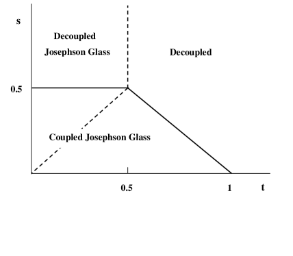
Figure 1: Phase diagram. Full lines are decoupling lines where the Josephson coupling vanishes. The upper dashed line is a depinning transition where the Josephson glass parameter vanishes; the lower dashed line is either a 1st order line or a crossover into a weaker JG phase, i.e. weaker pinning.

Finally, for $\Delta_{0}=0$ a replica symmetric solution is valid at $s<t$, which upon using Eqs. (28, 47) becomes

$$\frac{z}{\Delta_{c}}=(\frac{E_{J}}{Td\Delta_{c}}e^{-s-\mbox{$\frac{1}{2}$}C_{1}})^{\frac{1}{1-s-t}}.$$ (52)

Thus $s+t=1$ for $s<\mbox{$\frac{1}{2}$}$ defines a ”thermal” decoupling transition.

The interpretation of the phase diagram needs to be supplemented by a few observations from an RG analysis. The RSB results above coincide with those of a 2D model where the parameters $t,s$ of the 3d system, as suitable $k$ averages (Eqs. 37,49), correspond to Hamiltonian parameters of the 2D system H3 . With this correspondence in mind, we infer next some qualitative modifications by using the 2D RG equations H3 ; Scheidl , Eq. (II). Note first that in a coupled phase $z$ is RG relevant and therefore $E_{v}$, which is generated to order $z^{2}$, is finite too, hence a weak glass phase is expected also in the regime $s<t<1-s$; this weak glass order is not captured by the RSB solution. The line $t=s$ for $s<\mbox{$\frac{1}{2}$}$ can therefore be either a 1st order transition or a crossover line. RG suggests (Eq. II) this crossover line at $t=\mbox{$\frac{1}{2}$}$: at $t<\mbox{$\frac{1}{2}$}$ RG yields $E_{v}$ which is largely independent of $z$, hence a strong JG order, while at $t>\mbox{$\frac{1}{2}$}$ RG generates $E_{v}\sim z^{2}$ with a weak JG order. The stability of the RSB solution shows that in fact this line, which is either 1st order or a crossover, is at $t=s$.

The RG, shows also a disorder induced decoupling, since Eq. (II) has a fixed point with $u^{*}=0$ and $v^{*}=(1-2t)/\gamma^{\prime}t$, stable at $t<\mbox{$\frac{1}{2}$}$ and strong disorder. Note that for this solution $s\sim\ln\xi$ increases with scale $\xi$, hence the correlator $\Gamma(r)=\langle\cos b_{n}^{\alpha}(\mbox{${\bf r}$})\cos b_{n}^{\alpha}(0)\rangle$ which by RSB decays as $r^{-2-4s}$ is actually decaying faster as $\ln\Gamma(r)\sim-\ln^{2}r$. Explicit solution of the 2D RG equations Scheidl found indeed a phase diagram very similar to that in Ref. H3, or in Fig. 1.

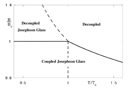
Figure 2: Phase diagram in terms of field and temperature. Full lines are decoupling lines [$B=B_{0}$ and $B=2B_{0}T_{0}/(T+T_{0})$] where the Josephson coupling vanishes. The upper dashed line is a depinning transition ($T=B_{0}T_{0}/B$) where the Josephson glass parameter vanishes; the lower dashed line ($T=T_{0}$) is either a 1st order transition or a crossover into weaker pinning.

The phase diagram, shown in Fig. 1, has three phase transition lines and a line which is either a 1st order or a crossover line. All these lines meet at a multicritical point $s=t=1/2$. We interpret the transition where $\Delta_{0}$ vanishes as a depinning transition, i.e. the JG order parameter provides an additional pinning to that from the Bragg glass. The phase diagram has then a decoupling line which crosses a depinning line at the multicritical point. The decoupling line has a disorder driven section, $s=\mbox{$\frac{1}{2}$}$ at $t<\mbox{$\frac{1}{2}$}$.

The phase diagram in terms of field and temperature is derived by defining $B_{0},T_{0}$ as the field and temperature value of the multicritical point and is shown in Fig. 2. $B_{0}$ is determined by the disorder strength via $s=\mbox{$\frac{1}{2}$}$ while $T_{0}=\mbox{$\frac{1}{2}$}T_{d}^{0}(a=\sqrt{B_{0}/\phi_{0}})$ (Eq. 7). Hence $s=B/2B_{0}$ and $t=TB/T_{0}B_{0}$, up to $\ln B$ terms. Since s increases with $B$ the $s=\mbox{$\frac{1}{2}$}$ line defines a decoupling transition from a coupled JG phase at low $B$ to a decoupled JG phase at high fields.

The coupled JG phase at $B<B_{0}$ goes through either a 1st order or a crossover line at $t=s$, i.e. at $T=T_{0}$ (up to $\ln B$ factors). Therefore at $T>T_{0}$ the glass parameter $\Delta_{0}$ is significantly reduced implying depinning, a change from strong to weak pinning. The decoupled JG phase undergoes a depinning transition into a decoupled phase at $T=B_{0}T_{0}/B$. Note that all phases, even the high $T$ decoupled one, are Bragg glass phases of the flux lattice; in the decoupled phase the lattice is maintained by the interlayer electromagnetic coupling.

The JG coupled phase at $T>T_{0}$ undergoes a decoupling transition at $t=1-s$, i.e. $B=2B_{0}T_{0}/(T+T_{0})$. This transition is continuous; the variational method of the pure system has been formally extended to higher $J/T$ and found to be of first order Daemen . As shown in the companion article GH , the transition remains 2nd order when proper 2nd order RG is employed. Disorder, however, leads to an apparent discontinuity near decoupling, as discussed in the next section.

IV Domain sizes

In this section we estimate various domain sizes and evaluate displacement fluctuations which identify these sizes. Remarkably, the expressions for the domain sizes are confirmed (up to numerical prefactors) by BG solutions (Appendices A-C). The nonsingular phase, which was irrelevant for the purpose of the phase diagram in section III, is essential now.

To appreciate the effect of the nonsingular phase $\theta$, we briefly review the derivation of the transverse tilt modulus $c_{44}$ of a pure flux lattice GH2 . The Josephson phase involves the contribution of pancake fluctuations via $b_{n}(\mbox{${\bf r}$})$ as well as a nonsingular phase, with the Hamiltonian Eq. (15). To identify $c_{44}$ we expand the Josephson coupling to 2nd order in ${\tilde{b}}(\mbox{${\bf q}$},k)=b(\mbox{${\bf q}$},k)+\theta(\mbox{${\bf q}$},k)$,

$${\cal H}_{pure}/T= \mbox{$\frac{1}{2}$}\sum_{q,k}\{[G_{f}^{-1}(q,k)+\frac{E_{J}}{Td}]\,\left|\,{\tilde{b}}(\mbox{${\bf q}$},k)-b(\mbox{${\bf q}$},k)\frac{G_{f}^{-1}(q,k)}{G_{f}^{-1}(q,k)+\frac{E_{J}}{Td}}\,\right|^{2}+$$ (53)

$$\frac{G_{f}^{-1}(q,k)\frac{E_{J}}{Td}}{G_{f}^{-1}({\bf q},k)+\frac{E_{J}}{Td}}|b(\mbox{${\bf q}$},k)|^{2}+\mbox{$\frac{1}{2}$}c(q,k)|b(\mbox{${\bf q}$},k)|^{2}+O({\tilde{b}}^{4}(\mbox{${\bf q}$},k))\}\,.$$

The first term decouples from $b(\mbox{${\bf q}$},k)$ and with $|b(\mbox{${\bf q}$},k)|^{2}=(2\pi d^{2})^{2}k_{z}^{2}|u^{tr}(q,k)|^{2}/q^{2}$ (Eq. 3) we identify GK ; Sudbo ; GH2

$$c_{44}(q,k)=c_{44}^{0}(k)+\frac{B^{2}}{4\pi}\frac{1}{1+\lambda_{c}^{2}q^{2}+\lambda_{ab}^{2}k^{2}}+\frac{2B\phi_{0}}{(8\pi\lambda_{c})^{2}}\ln(a^{2}/4\pi\xi_{0}^{2})$$ (54)

where $\lambda_{c}^{2}=\lambda_{ab}^{2}\tau/(4\pi d^{2}E_{J})$; the last term is from reducing high momenta of the 2nd term of (53) into the 1st Brilluin zone.

The second term of $c_{44}(q,k)$ is peculiar: at $q\neq 0$ it vanishes when $E_{J}$ vanishes and $\lambda_{c}\rightarrow\infty$, as it should. However, at $q=0$ this term seems to survive even if $\lambda_{c}\rightarrow\infty$. The origin of this peculiarity is that the harmonic expansion of the Josephson cosine term which identifies $c_{44}$ failsGH2 when both $q,\,1/\lambda_{c}\rightarrow 0$. The shift in the 1st term of Eq. (53) identifies an expansion parameter GH2 with terms $\sim q^{2}k_{z}^{2}|u_{T}({\bf q},k)|^{2}/[q^{2}+\lambda_{c}^{-2}(1+\lambda_{ab}^{2}k_{z}^{2})]^{2}$, which diverge when both $q,1/\lambda_{c}\rightarrow 0$ and the expansion becomes invalid. In fact, the nonlinear cosine term replaces $E_{J}/Td$ by $z$ or $\lambda_{c}$ is replaced by a renormalized

$$\lambda_{c}^{R}=\sqrt{\lambda_{ab}^{2}\tau/(4\pi Td^{3}z)}$$ (55)

which diverges at decoupling. Hence usual elasticity at $q,1/\lambda_{c}^{R}\rightarrow 0$ near decoupling is ill defined.

The Bragg glass domain size $R_{BG}$ (parallel to the layers) sets a scale for the relevant $q$ values. When $R_{BG}>\lambda_{c}^{R}$ the tilt modulus is large, containing the $B^{2}/4\pi$ term of Eq. (54). However, as decoupling at the field $B_{0}$ is approached $\lambda_{c}^{R}$ diverges so that when $R_{BG}<\lambda_{c}^{R}\,$ Eq. (54) fails to describe $c_{44}$ on the scale of $q\approx 1/R_{BG}$. This defines an anharmonic crossover regime where usual elasticity cannot be used to derive Bragg glass properties. Finally, at $B>B_{0}$ elasticity is restored and $c_{44}$ is reduced to the first term in Eq. (54). The main interest is in the regime of strong fields, i.e. $a\lesssim 2\lambda_{ab}$ where $T_{0}\ll\tau$ is below melting. Thus at $B<B_{0}$ and for sufficiently large domains the second term in Eq. (54) dominates and $c_{44}=B^{2}/4\pi$ while at $B>B_{0}$ only the magnetic coupling survives $c_{44}=c_{44}^{0}(k)$ which at $ka\ll 1$ becomes $\tau/(32\pi\lambda_{ab}^{2}d)$. Hence there is an apparent discontinuity,

$$c_{44} = \pi\lambda_{ab}^{2}\tau/da^{4}\hskip 51.21495pt\lambda_{c}^{R}<R_{BG}$$ (56)

$$= \tau/(32\pi\lambda_{ab}^{2}d)\hskip 42.67912pt\lambda_{c}^{R}=\infty$$ (57)

Thus $c_{44}$ is reduced within the anharmonic regime by the small factor

$$\epsilon=a^{4}/(32\pi^{2}\lambda_{ab}^{4})\,.$$ (58)

The apparent discontinuity in $c_{44}$ affects also the domain sizes which can be estimated by a dimensional argument LO ; Giamarchi . Consider the tilt $c_{44}$ and shear $c_{66}$ terms of the elasticity Hamiltonian for the displacement ${\bf u}({\bf r})$ and its transverse component ${\bf u}_{T}({\bf r})$. Rescaling parallel and perpendicular lengths yields an isotropic form Blatter ; Natterman , which together with the pinning energy (18) yield (ignoring elasticity of longitudinal displacements)

$${\cal H}=\int d^{3}r\{\mbox{$\frac{1}{2}$}c_{44}^{1/3}c_{66}^{2/3}[{\mbox{\boldmath$\nabla$}}u_{T}({\bf r})]^{2}-(\xi_{0}^{2}/a^{2}d)U_{pin}({\bf r})\sum_{{\bf Q}}\cos{\bf Q}\cdot[\mbox{${\bf r}$}-{\bf u}({\bf r})]\}$$ (59)

where the disorder coupling to ${\mbox{\boldmath$\nabla$}}u_{T}({\bf r})$ is neglected. To estimate the energy gain from disorder we consider the overlap of the disorder energy between two configurations ${\bf u}({\bf r})$ and ${\bf u}^{\prime}({\bf r})$ which are solutions for two realizations of the random potential Blatter ; this overlap is a measure of the energy variance in configuration space. The ${\bf r}$ integration leads to a single ${\bf Q}$ sum so that the variance is $\sim\sum_{{\bf Q}}\cos{\bf Q}\cdot[{\bf u}({\bf r})-{\bf u}^{\prime}({\bf r})]$. Each of ${\bf u}({\bf r})$ and ${\bf u}^{\prime}({\bf r})$ has fluctuations $\langle u^{2}\rangle\approx\langle u_{T}^{2}\rangle$ in a domain of size $R^{\prime}$ so that the ${\bf Q}$ sum is cutoff by $Q\lesssim\langle u_{T}^{2}\rangle^{-1/2}$. Below this cutoff the cosine can be expanded and summed so that averaging Eq. (59) yields

$$\langle H\rangle/R^{\prime 3}=\mbox{$\frac{1}{2}$}c_{44}^{1/3}c_{66}^{2/3}\langle u_{T}^{2}\rangle R^{\prime-2}-{\bar{U}}^{1/2}\xi_{0}^{2}/[a^{2}d\langle u_{T}^{2}\rangle R^{\prime 3}]^{1/2}\,.$$ (60)

Minimizing with respect to $R^{\prime}$ yields $R^{\prime}\sim\langle u_{T}^{2}\rangle^{3}$, i.e. the Flory exponent Giamarchi . This exponent is not exact; the more accurate statement, shown within the BG solution Giamarchi , is that the disorder averaged correlation ${\tilde{B}}(R^{\prime})=\langle[u_{T}({\bf R}^{\prime})-u_{T}(0)]^{2}\rangle\sim R^{\prime 1/3}$ is a quantitatively correct description in the range between the pinning length $R_{p}$ where ${\tilde{B}}(R_{p})=\xi_{0}^{2}$ and $R_{BG}$ where ${\tilde{B}}(R_{BG})=a^{2}$. The fluctuations $\langle u_{T}^{2}\rangle$ on scale $R^{\prime}$ in the dimensional argument correspond then to ${\tilde{B}}(R^{\prime})$.

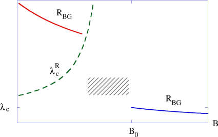
Figure 3: Bragg glass domain size $R_{BG}$ parallel to the layers and the renormalized London length perpendicular to the layers $\lambda_{c}^{R}$; the latter diverges at the decoupling field $B_{0}$. $R_{BG}$ can be found from elasticity for $B<B_{0}$ only if $R_{BG}>\lambda_{c}^{R}$; otherwise, as in the hatched region, the elastic tilt modulus is ill defined.

The domain size parallel to the layers is, from minimizing Eq. (60), (up to $\ln(a/d)$ and a numerical prefactor)

$$R^{+} \approx (\lambda_{ab}/a)^{5}\langle u_{T}^{2}\rangle^{3}/(s\xi_{0}^{4}d)\hskip 56.9055pt\lambda_{c}^{R}<R^{+}$$

$$R^{-} \approx (\lambda_{ab}/a)^{3}\langle u_{T}^{2}\rangle^{3}/(4\pi s\xi_{0}^{4}d)\hskip 42.67912pt\lambda_{c}^{R}=\infty\,.$$ (61)

The pinning length $R=R_{p}$ is given by Eq. (IV) with $\langle u_{T}^{2}\rangle\approx\xi_{0}^{2}$. The condition $\lambda_{c}^{R}<R_{p}^{+}$ is not valid for BSCCO parameters; to allow for large pinning domains one needs either $a\ll\lambda_{ab}$ or to allow for domains with a somewhat larger fluctuations in $\langle u_{T}^{2}\rangle$; the latter increases $R_{p}$ very rapidly since it increases with the 6-th power of $u_{T}$. The critical current can now be estimated Blatter ; LO by balancing the Lorenz force $j_{c}BR^{3}/c$ with the pinning force $\langle H\rangle/\xi_{0}$ (evaluated at the minimum of Eq. (60)), leading to $j_{c}\sim 1/c_{44}$. Increasing the field within the anharmonic regime decreases $c_{44}$ by the factor $\epsilon$ so that $j_{c}$ is enhanced by a $1/\epsilon$ factor which is significant when $a\lesssim\lambda_{ab}$.

A second length scale $R=R_{BG}$ is identified by Eq. (IV) with the fluctuations $\langle u_{T}^{2}\rangle\approx a^{2}$. The proper definition of $R_{BG}$ is the scale for the onset of the $\ln r$ form for the displacement correlation function, as inferred in Eq. (98) or (B). It is remarkable that Eq. (IV) gives the correct form for for $R_{BG}$, up to a numerical prefactor, i.e. Eqs. (98, B). Eq. (IV) shows that $R_{BG}$ is reduced by $\epsilon^{1/2}$ through the anharmonic regime. The onset of the anharmonic regime is at $R_{BG}^{+}\approx\lambda_{c}^{R}$, i.e.

$$\lambda_{c}^{R}\approx 10^{-3}\frac{a\mbox{${\lambda_{ab}}$}^{5}}{sd\xi_{0}^{4}}$$ (62)

with a numerical prefactor from the BG solution (Eqs. 98, B). For BSCCO or YBCO parameters at $s\approx\mbox{$\frac{1}{2}$}$ this reduces to $\lambda_{c}^{R}/\mbox{${\lambda_{ab}}$}\approx 10^{5}$, i.e. the initial anisotropy of $\lambda_{c}/\mbox{${\lambda_{ab}}$}=10-100$ has to increase to $\approx 10^{5}$. Since $z$ is exponentially renormalized (Eqs. 50, 52) this anharmonic range may be observable.

Fig. 3 illustrates the lengths $R_{BG}$ and $\lambda_{c}^{R}$, demonstrating the anharmonic regime within which $R_{BG}$ has a significant drop and correspondingly $j_{c}$ has an apparent jump. Note that even in the decoupled phase ($B>B_{0}$) $R_{BG}$ is large for typical type II superconductors, $R_{BG}\approx\lambda_{ab}^{3}a^{3}/(4\pi s\xi_{0}^{4}d)\gg a$, consistent with a decoupling transition within the Bragg glass phase, i.e. below a melting transition.

The solution of section III can also be extended to include the nonsingular phase. Since disorder is linearized, the pinning length $R_{p}$ can be determined, though the BG length cannot. Appendix C develops this solution and shows that in the coupled phase $R_{p}$ coincides with $R^{+}$ Eq. (IV) (with $\langle u_{T}^{2}\rangle\approx\xi_{0}^{2}$), up to a numerical prefactor.

The main result is then that the fluctuations in $u_{T}(r)$ behave with an effective $c_{44}$ which is large when $q<1/\lambda_{c}^{R}$ (Eq. (56)), i.e. for domain sizes $R_{BG}>\lambda_{c}^{R}$, while for $z=0$ $c_{44}$ is reduced (Eq. (57)). While the condition $\lambda_{c}^{R}<R_{p}^{+}$ in Eq. (IV) is not valid for BSCCO (the pinning domains are likely to be two dimensional) our results for the anharmonic regime itself in terms of the much larger $R_{BG}$ are valid. The existence of a narrow anharmonic regime leads to an apparent jump in $c_{44}$ which possibly affects the critical current.

In the anharmonic region below decoupling (see Fig. 3) where $R_{BG}<\lambda_{c}^{R}$ a more complete form [e.g. Eq. (120)] is required to interpolate between the limiting forms of $c_{44}$. However, a method relying on an effective harmonic theory, such as RSB, is suspect within the anharmonic regime, since the system has no effective elastic constants. Furthermore, RSB signals this deficiency by producing a $ln^{2}z$ term, precisely in the the anharmonic regime found here, as shown in Appendices A and B.

V Josephson Plasma resonance

Josephson plasma resonance provides extremely useful data for identifying phases of vortex matter Matsuda ; Koshelev ; Shibauchi ; Matsuda2 . In particular a jump in the resonance frequency $\omega_{pl}$ has shown Shibauchi ; Matsuda2 that the Josephson coupling is strongly modified at the second peak transition. In this section we derive $\omega_{pl}$ in the ordered phases and also consider the fluctuation contribution in the disordered phase. The Josephson plasma frequency is given by Koshelev (see also the companion article GH section V)

$$\omega_{pl}^{2}=\frac{16\pi e^{2}dE_{J}}{\epsilon_{0}\hbar^{2}}\langle\cos b\rangle$$ (63)

where $\epsilon_{0}$ is a dielectric constant. The task is then to evaluate the thermodynamic average $\langle\cos b\rangle$.

Consider first the ordered phases where at least one of $z$ and $\Delta_{0}$ is finite. We start by evaluating ${\cal F}_{var}$ of Eq. (26) for a general one step RSB, recover the solution of section III, and then identify $\langle\cos b\rangle$. This derivation is needed so that the free energy itself can be evaluated, and from the latter $\langle\cos b\rangle$ is inferred. The self mass term $\sigma_{\alpha,\beta}$ of Eq. (27) is written for a one step solution in the form

$${\hat{\sigma}}=\sigma_{0}{\hat{L}}+(\sigma_{1}-\sigma_{0}){\hat{C}}-[\sigma_{0}n+(\sigma_{1}-\sigma_{0})m]{\hat{I}}$$ (64)

where ${\hat{L}}_{\alpha,\beta}=1$ and ${\hat{C}}$ has $1$ elements in blocks of size $m\times m$ sitting consecutively along the diagonal, and $0$ elements otherwise. For $n\rightarrow 0$ we identify $(\sigma_{1}-\sigma_{0})m=\Delta_{0}$ so that

$${\hat{G}}(q,k)=[(c(q,k)q^{2}+z+\Delta_{0}){\hat{I}}+(-s_{0}\frac{q^{2}}{k_{z}^{2}}-\sigma_{0}){\hat{L}}-\frac{\Delta_{0}}{m}{\hat{C}}]^{-1}\equiv\alpha{\hat{I}}+\beta{\hat{L}}+\gamma{\hat{C}}\,.$$ (65)

It is straightforward to identify the coefficients of the inverse matrix

$$\alpha(q,k) = \frac{1}{c(q,k)q^{2}+z+\Delta_{0}}\,,\qquad\qquad\alpha=\sum_{\mbox{${\bf q}$},k}\alpha(q,k)=2t\ln\frac{\Delta_{c}}{z+\Delta_{0}}+C_{1}$$

$$\beta(q,k) = \frac{s_{0}\frac{q^{2}}{k_{z}^{2}}+\sigma_{0}}{[c(q,k)q^{2}+z]^{2}}\,,\qquad\qquad\beta=\sum_{\mbox{${\bf q}$},k}\beta(q,k)=2s(\ln\frac{\Delta_{c}}{z}-1)+\frac{2t\sigma_{0}}{z}$$

$$\gamma(q,k) = -\frac{1}{m}[\alpha(q,k)-\frac{1}{c(q,k)q^{2}+z}]\,,\qquad\gamma=\sum_{\mbox{${\bf q}$},k}\gamma(q,k)=\frac{2t}{m}\ln\frac{z+\Delta_{0}}{z}$$ (66)

where the form of Eq. (49) is used for $I(z)$ in the 2nd line. The definition of ${\hat{\sigma}}$ identifies $\sigma_{1}=2E_{v}e^{-\alpha}/d$ and $\sigma_{0}=2E_{v}e^{-\alpha-\gamma}/d$. We follow a similar algebra in section IV of Ref. H3, to evaluate the free energy density per replica as

$$f(m,z,\Delta_{0})=f_{0}+(1-\frac{1}{m}t\Delta_{0}+(1+\frac{s}{t})tz-\frac{E_{v}}{Td}(2t-m)e^{-\alpha-\gamma}+\frac{E_{v}}{Td}(1-m)e^{\alpha}-\frac{E_{J}}{Td}e^{-\mbox{$\frac{1}{2}$}(\alpha+\beta+\gamma)}$$ (67)

where $f_{0}$ is $m$, $z$ and $\Delta_{0}$ independent. Minimizing $f(m,z,\Delta_{0})$ yields $m=2t$ and Eqs. (III,43,50)for $\sigma_{0},\sigma_{1},z+\Delta_{0}$ and $z$. A replica symmetric solution is also possible with $\Delta_{0}=0$ leading to Eq. (52). The free energy at minimum is

$$f_{min}=f_{0}+(t-1+\frac{1}{4t})(\Delta_{0}+z)+(s-\mbox{$\frac{1}{2}$})z\,.$$ (68)

The Hamiltonian Eq. (12) shows that $\langle\cos b\rangle=-Td(\partial f/\partial E_{J})$. As discussed below Eq. (52) $E_{v}$ is generated from $E_{J}$ in 2nd order RG so that $E_{v}\sim E_{J}^{2}$ initially, while $E_{v}$ is RG relevant at $t<\mbox{$\frac{1}{2}$}$, so that its value which is to be used by the variational scheme is more weakly $E_{J}$ dependent. We assume then $E_{v}\sim E_{J}^{\kappa}$ with $0<\kappa<2$. Hence in the $\Delta_{0}\neq 0$ phases

$$\frac{\partial(z+\Delta_{0})}{\partial E_{J}} = \frac{\kappa(z+\Delta_{0})}{E_{J}(1-2t)}$$

$$\frac{\partial z}{\partial E_{J}} = \frac{(2-\kappa)}{(1-2s)E_{J}}$$

$$\langle\cos b\rangle = -\kappa(1-2t)\frac{z+\Delta_{0}}{z_{bare}}+(1-\mbox{$\frac{1}{2}$}\kappa)\frac{z}{z_{bare}}$$ (69)

where $z_{bare}=E_{J}/Td$ is the bare value of $z$. For the $\Delta_{0}=0$ phase

$$\frac{\partial z}{\partial E_{J}} = \frac{z}{(1-t-s)E_{J}}$$

$$\langle\cos b\rangle = \frac{z}{z_{bare}}$$ (70)

so that at $T=s=0$ the order is maximal, $\langle\cos b\rangle=1$.

These results show that the JG order produces a negative contribution to $\langle\cos b\rangle$ so that when crossing a depinning line $\langle\cos b\rangle$ is enhanced by the $\sim\kappa$ terms in Eq. (V). Since $\Delta_{0}$ is continuous, the jump at depinning is $\kappa(\frac{3}{2}-2t)z/z_{bare}$. As discusses in section III, the depinning in the lower part of Fig. 1 is not a strict phase transition, but rather a crossover line, hence we expect a smeared jump of $\langle\cos b\rangle$. An observation of a $\langle\cos b\rangle$ enhancement when crossing the lower depinning line at $T\approx T_{0}$ ($B<B_{0}$) would be a clear signature that depinning relates to JG order. The actual enhancement depends on $\kappa$, for which we do not have a precise derivation.

Near the decoupling transitions, the presence of anharmonic regimes, shown in section IV, lead to an apparent jump in $\langle\cos b\rangle$. This jump relates to the $z$ terms in (V) and also depends on the fluctuation contribution which is considered next.

We proceed to evaluate fluctuation contribution when $\langle\cos b\rangle$ is small. As shown by Koshelev Koshelev the local $\langle\cos b_{n}(r)\rangle$ is finite even at high temperatures, e.g. above the decoupling transition. The high temperature expansion, while formally ill defined, does reproduce the RG results for $\langle\cos b\rangle$, as shown in section III of the companion article GH . The high temperature expansion yields

$$\langle\cos b_{n}(r)\rangle = (E_{J}/2T)\int d^{2}r\exp[-A(r)]$$

$$A(r) = \sum_{{\bf q},k}(1-\cos{\bf q}\cdot{\bf r})\langle|b^{\alpha}({\bf q},k)|^{2}\rangle\,.$$ (71)

For $r^{2}>1/q_{u}^{2}$ we can use the form (III) with $z$ replaced by a cutoff $c(k)/r^{2}$ while for $r<1/q_{u}$ we expand $1-\cos\mbox{${\bf q}$}\cdot\mbox{${\bf r}$}\rightarrow\frac{1}{4}q^{2}r^{2}$, hence

$$A(r) = 4(s+t)\ln(q_{u}r)\qquad r>1/q_{u}$$ (72)

$$= \mbox{$\frac{1}{2}$}(s+t)q_{u}^{2}r^{2}\qquad r<1/q_{u}\,.$$

The two regimes in Eq. (72) give comparable results, though the $r>1/q_{u}$ is larger near the transition and reproduces the form of the RG result, as discussed in section III of the companion article GH . The latter yields, in terms of the multicritical point coordinates (up to $\ln B$ terms),

$$\langle\cos b\rangle\approx\frac{\pi E_{J}\lambda_{ab}^{2}}{8\ln(a/d)}\cdot\frac{B_{0}T_{0}}{T(BT_{0}+BT-B_{0}T_{0})}\,.$$ (73)

Well above decoupling at $s+t\gg\frac{1}{2}$ we obtain $\langle\cos b\rangle\sim[BT(T+T_{0})]^{-1}$. A $1/BT$ dependence has been obtained by Koshelev Koshelev with a weakly temperature dependent prefactor for an XY model, i.e. infinite $\lambda_{ab}$ model. This result corresponds, in fact, to the melted, or liquid phase GH . Data on BSCCO Matsuda has shown that $\langle\cos\tilde{b}_{n}(r)\rangle\sim B^{-0.8}T^{-1}$ in reasonable agreement with the $1/BT$ form. The present result shows that in the decoupled phase, below melting, $\omega_{pl}\sim[BT(T+T_{0})]^{-1}$, or the form (73) near decoupling. This distinct temperature dependence can be used to identify the decoupled phase.

As decoupling is crossed, we expect a positive fluctuation term to compensate the negative contribution of the JG order. Thus the forms (V,V) can be used for the jumps of $\langle\cos b\rangle$ across depinning or decoupling, while (V) is valid in the high temperature or high field regime where $\langle\cos b\rangle$ is small.

VI Discussion

The present work exhibits the JG order parameter as well as the decoupling transition with disorder. We discuss now our proposal for each of the 4 transition lines emanating from the multi-critical point (Fig. 2) and compare with experimental data.

Consider first the decoupling transition within the JG phase at $B=B_{0}$, $T<T_{0}$. We have shown that RSB methods are suspect within a narrow region near decoupling, where usual elasticity is ill defined (Fig. 3). RSB identifies this as a $\ln^{2}z$ divergence in $A_{\alpha}$ which renormalizes $z$ (Eq. 28). This can be thought of as a disorder term $s_{eff}\sim\ln z$ with a diverging $s_{eff}$. The consequence is an apparent discontinuity, or even an intrinsic 1st order transition, driven by disorder.

This decoupling transition is consistent with the main features of the second peak transition: (i) decoupling field being weakly $T$ dependent Kes ; Khaykovich1 ; Khaykovich2 ; Deligiannis , (ii) decoupling field decreasing with impurity concentration Khaykovich1 , (ii) an apparent jump in the critical current Kes ; Khaykovich1 ; Khaykovich2 ; Deligiannis ; Giller ; Higgins ; Marley ; Bruynseraede (iv) decrease in the c axis critical current Ooi and (v) a jump in the Josephson plasma resonance Shibauchi ; Matsuda2 . The anharmonic region near decoupling leads to an apparent reduction in $c_{44}$. The reduction in $c_{44}$ and the resulting reduction in domain sizes account qualitatively for the enhanced $j_{c}$. We do not attempt a quantitative fit; in fact, the measured magnetization changes (and inferred $j_{c}$) at the second peak decrease with temperature due to the strongly temperature dependent relaxation rates Yeshurun , approaching the much smaller equilibrium magnetizations.

The nature of the phase at fields above the second peak line has not been conclusively settled. This work proposes that it is a BG phase where the domain sizes have been reduced by $\sqrt{\epsilon}=a^{2}/(4\pi\sqrt{2}\mbox{${\lambda_{ab}}$}^{2})$. Experimentally, the smooth connection of the second peak with the 1st order line Avraham suggests that it is a single ”order-disorder” line of common origin, e.g. a melting line. However, the presence of a depinning line that crosses the ”order-disorder” line has been seen by numerous experiments Fuchs ; Kopelevich ; Dewhurst ; Ooi . The crossing of this depinning line with the ”order-disorder” line, separates the latter into a disorder driven second peak part within a pinned regime and into a thermally driven part in a depinned, or more weakly pinned regime. This depinning line corresponds to the onset of a Josephson glass order, as suggested below.

Consider next the decoupling line at $T>T_{0}$. This corresponds to the 1st order transition, which is considered as a melting line Kes ; Avraham . However, neutron data Forgan has shown a reentrant behavior in the $600-10^{3}G$ range with positional correlations increasing with temperature. It is possible then that near the multi-critical point the 1st order line is a decoupling line. At higher temperatures decoupling then merges into a melting line.

The 3rd transition line is a transition within the JG order at $T=T_{0}$, $B<B_{0}$ into a weaker JG at $T>T_{0}$. A depinning line which is almost vertical at $T\approx T_{0}$ was indeed observed Fuchs ; Kopelevich ; Dewhurst ; Ooi . We note in particular the c axis critical current Ooi which shows a decrease on the high temperature side of the depinning line. The thermodynamic critical current is proportional to the renormalized $z$ that changes from the weakly $T$ dependent Eq. (51) at $T<T_{0}$ to the strong exponential decrease with $T$ in Eq. (53) at $T>T_{0}$ , consistent with the data. At $T>T_{0}$ we also expect a sharp enhancement of the Josephson plasma resonance, which is an additional tool for identifying the JG order parameter.

The final 4th line is a depinning line at $T=B_{0}T_{0}/B$, $B>B_{0}$ corresponding to a depinning line as observed in BSCCO by current distribution data Fuchs , vibration reed Kopelevich , magnetization Dewhurst and c axis critical current data Ooi . This line is more difficult to detect by Josephson plasma resonance since its frequency varies continuously, with discontinuities in derivatives. In the decoupled phases (with or without JG order), where $\langle\cos b\rangle$ is small, we expect the fluctuation form Eq. (73).

We have assumed throughout that our transition lines are well below melting. Thermal melting is discussed below Eq. (7) while here we estimate the disorder induced melting field. We assume a Lindeman criterion such that the fluctuations in the decoupled phase on scale $R^{-}=a$ are $\langle u_{T}^{2}\rangle=c_{L}^{2}a^{2}$, with $c_{L}=0.15$ a conventional Lindeman number²¹. Using Eq. (IV) with a prefactor as identified by Eq. (98) yields a melting field of $B_{m}\approx 10^{-2}c_{L}^{3}\sqrt{2B_{0}B_{\lambda}\lambda_{ab}^{5}/d\xi_{0}^{4}}$ where $B_{\lambda}=\phi_{0}/\lambda_{ab}^{2}$. With BSCCO parameters the condition $B_{m}>B_{0}$ is satisfied if $B_{0}\lesssim 50B_{\lambda}$, hence with the second peak field of $B_{0}\approx B_{\lambda}\approx 500G$ disorder induced melting is expected at a higher field.

In conclusion, we have found a phase diagram which is remarkably close to the experimental one Kes ; Khaykovich1 ; Khaykovich2 ; Deligiannis ; Fuchs ; Dewhurst ; Ooi , having a multicritical point and providing a fundamental interpretation of both the second peak transition and the more recently observed depinning transitions.

Note Added

In a recent work [H. Beidenkopf, N. Avraham, Y. Myasoedov, H. Shtrikman, E. Zeldov, and T. Tamegai (unpublished)] the depinning transitions were identified by relaxed magnetization data as equilibrium transitions. Both transitions at fields below and above the multicritical point were identified and suggested to be equilibrium glass transitions.

Acknowledgments: We thank E. Zeldov, D. T. Fuchs and P. Le Doussal for most valuable and stimulating discussions. This research was supported by THE ISRAEL SCIENCE FOUNDATION founded by the Israel Academy of Sciences and Humanities.

Appendix A Bragg and Josephson glasses

This section studies nonlinearities due to both disorder and Josephson coupling leading to two glass order parameters – the Josephson glass (JG) and the Bragg glass (BG); the non-singular phase is neglected. In particular an equivalent term to the integral $I(z)$ (Eq. 45) is identified and is shown to be convergent at $k\rightarrow 0$.

We consider the full Hamiltonian Eq. (21), which by neglecting the nonsingular phase becomes

$${\cal H}/T=\mbox{$\frac{1}{2}$}\sum_{\mbox{${\bf q}$},k,\alpha}(c^{\prime}\frac{q^{4}}{k_{z}^{2}}+c(k)q^{2})|b^{\alpha}(\mbox{${\bf q}$},k)|^{2}-\frac{E_{J}}{T}\sum_{n;\alpha}\int d^{2}r\,\cos b_{n}^{\alpha}({\bf r})$$

$$-\frac{E_{v}}{T}\sum_{n;\alpha\neq\beta}\int d^{2}r\cos[b_{n}^{\alpha}({\bf r})-b_{n}^{\beta}({\bf r})]-\frac{g_{0}}{a^{2}}\sum_{\alpha\neq\beta,n}\int d^{2}r\cos[\mbox{${\bf Q}$}\cdot(\mbox{${\bf u}$}^{n,\alpha}(\mbox{${\bf r}$})-\mbox{${\bf u}$}^{n,\beta}(\mbox{${\bf r}$}))]$$ (74)

The average of the disorder term over the variational Hamiltonian (23) ${\cal H}_{0}$ yields

$$\langle\cos[\mbox{${\bf Q}$}\cdot(\mbox{${\bf u}$}^{n,\alpha}(\mbox{${\bf r}$})-\mbox{${\bf u}$}^{n,\beta}(\mbox{${\bf r}$}))]\rangle=\exp\{-\frac{a^{2}}{2d^{2}}\sum_{\mbox{${\bf q}$},k}\frac{q^{2}}{k_{z}^{2}}[G_{\alpha\alpha}(q,k)-G_{\alpha\beta}(q,k)]\}\,.$$ (75)

We assume for simplicity a square lattice, $Q=2\pi/a$, otherwise a factor $(aQ/2\pi)^{2}$ is needed in the exponent; there are then 4 shortest ${\bf Q}$ terms in Eq. (A). The variational equation for $G_{\alpha,\beta}^{-1}(q,k)$, Eq. (27), has now an additional self energy term $\sigma_{\alpha\beta}^{(1)}$ which allows for an additional RSB. Written as an equation for matrices in replica space, e.g. ${\hat{G}}$, we have

$${\hat{G}}^{-1}(q,k)=(c^{\prime}\frac{q^{4}}{k_{z}^{2}}+c(k)q^{2}+z){\hat{I}}-{\hat{\sigma}}_{2}-\frac{q^{2}}{k_{z}^{2}}{\hat{\sigma}}_{1}\,.$$ (76)

When $({\hat{\sigma}}_{1})_{\alpha\beta}=1$, i.e. no RSB, the previous form (27) is recovered. The variational ${\cal F}_{var}$ (26) has now a term $\sim\exp[-\mbox{$\frac{1}{2}$}B_{\alpha\beta}^{(1)}]$ (instead of the $s_{0}$ term) where

$$B_{\alpha\beta}^{(1)}=\frac{a^{2}}{d^{2}}\sum_{\mbox{${\bf q}$},k}\frac{q^{2}}{k_{z}^{2}}[G_{\alpha\alpha}(q,k)-G_{\alpha\beta}(q,k)]\,.$$ (77)

The variation of this term identifies

$$\sigma_{\alpha\beta}^{(1)}=\frac{4g_{0}}{d^{3}}[e^{-\mbox{$\frac{1}{2}$}B_{\alpha\beta}^{(1)}}-\delta_{\alpha\beta}\sum_{\gamma}e^{-\mbox{$\frac{1}{2}$}B_{\alpha\gamma}^{(1)}}]$$ (78)

while $\sigma_{\alpha\beta}^{(2)}$ and $B_{\alpha\beta}^{(2)}$ have the previous forms (25, 29). In the hierarchical scheme $G^{-1}$ is represented by $[{\tilde{a}},a(u)]$ which are now given by

$${\tilde{a}} = c^{\prime}\frac{q^{4}}{k_{z}^{2}}+c(k)q^{2}+z-{\tilde{\sigma}}_{2}-{\tilde{\sigma}}_{1}\frac{q^{2}}{k_{z}^{2}}$$

$$a(u) = -\sigma_{2}(u)-\sigma_{1}(u)\frac{q^{2}}{k_{z}^{2}}\,.$$ (79)

The JG and BG order parameters which measure the degree of RSB are $\Delta_{1}(u),\Delta_{2}(u)$, respectively, where $\Delta_{i}(u)=u\sigma_{i}(u)-\int_{0}^{u}\sigma_{i}(v)dv$, $i=1,2$. Using the inversion (III) we can write

$$\mbox{$\frac{1}{2}$}B_{i}(u)=\frac{g_{i}(u)}{u}-\int_{u}^{1}\frac{g_{i}(v)}{v^{2}}dv\qquad i=1,2$$ (80)

where

$$g_{1}(u) = \frac{a^{2}}{2d^{2}}\sum_{\mbox{${\bf q}$},k}[c^{\prime}q^{2}+c(k)k_{z}^{2}+(z+\Delta_{2}(u))\frac{k_{z}^{2}}{q^{2}}+\Delta_{1}(u)]^{-1}$$

$$g_{2}(u) = \sum_{\mbox{${\bf q}$},k}[c^{\prime}\frac{q^{4}}{k_{z}^{2}}+c(k)q^{2}+z+\Delta_{2}(u)+\Delta_{1}(u)\frac{q^{2}}{k_{z}^{2}}]^{-1}\,.$$ (81)

As in Eq. (39), we find

$$\frac{\Delta_{i}^{\prime}(u)}{u}=-\frac{d}{du}[\frac{\Delta_{i}^{\prime}(u)}{g_{i}^{\prime}(u)}]\qquad i=1,2\,.$$ (82)

Consider first $g_{2}(u)$ which is dominated by $k\gg q$ so that the $c^{\prime}$ term produces just the cutoff $q_{u}$. The $q$ integration then yields Eq. (38) with $\Delta_{c}\rightarrow[c(k)+\Delta_{1}(u)/k_{z}^{2}]q_{u}^{2}$ in the logarithm. As above, we replace $k$ by $\pi/d$ in this logarithm since the $k$ integral is dominated by $k\approx\pi/d$ due to the significant softening of $c(k)$ near $k=\pi/d$. Hence the form $g_{2}(u)\sim\ln[z+\Delta_{2}(u)]$ is maintained and the solution, as in (40) is a one step function at $u=2t$.

To solve the equation for $\Delta_{1}(u)$ we simplify the form of $c(k)$ as

$$c(k) = c(0)\equiv c_{-}\qquad\qquad k<\frac{1}{a}$$ (83)

$$= c(\frac{\pi}{d})\frac{4}{d^{2}k_{z}^{2}}\qquad k>\frac{1}{a}$$

This form captures the significant dispersion of $c(k)$ with $c(\pi/d)\ll c(0)$ and allows analytic treatment of the potentially divergent $k\rightarrow 0$ integrals. The $k>\frac{1}{a}$ integration range in $g_{1}(u)$ has an integrand

$$[c^{\prime}q^{2}+\Delta_{1}(u)+c(\pi/d)(4/d^{2})+(z+\Delta_{2}(u))k_{z}^{2}/q^{2}]^{-1}$$

so that $c(\pi/d)(4/d^{2})\gg\Delta_{1}(u)$ provides a cutoff on the $q$ integration, i.e. $g_{1}(u)$ acquires a term independent of $\Delta_{1}(u)$. The $k<\frac{1}{a}$ integration has $c(0)/a^{2}\gg\Delta_{1}(u)$ so that after the $k$ integration

$$g_{1}(u)=\frac{a^{2}}{8\pi d^{2}}\int\frac{q^{2}dq}{\sqrt{(c^{\prime}q^{2}+\Delta_{1}(u))(c_{-}q^{2}+z+\Delta_{2}(u))}}+const\,.$$ (84)

$\Delta_{1}(u)$ varies between $\Delta_{1}(0)=0$ and $\Delta_{1}(u_{c})$ which depends on the disorder strength (see below); $\Delta_{1}(u)=\Delta_{1}(u_{c})$ is constant at $u>u_{c}$, being a valid solution of (82). As the decoupling transition is approached and $z\rightarrow 0$ the $q$ integration in (84) has distinct forms depending on the ratio of $\Delta_{1}(u)$ and $c^{\prime}z/c_{-}$. When $\Delta_{1}(u)<c^{\prime}z/c_{-}$ the dominant integration range is $\Delta_{1}(u)/c^{\prime}<q^{2}<z/c_{-}$ and the result for the derivative is

$$\frac{d}{d\Delta_{1}}g_{1}(\Delta_{1})=\frac{\alpha^{\prime}}{\sqrt{z}}\ln\Delta_{1}\qquad\alpha^{\prime}=\frac{a^{2}}{8\pi d^{2}c^{\prime 3/2}}\,.$$ (85)

Substituting in (82) yields $\Delta_{1}(u)\approx u\sqrt{z}/\alpha^{\prime}\ln^{2}u$ and with (80) we obtain [$C_{2}=g_{1}(u=0)$]

$$g_{1}(u) = C_{2}+\frac{u}{\ln u}+O(\frac{u}{\ln^{2}u})$$

$$\mbox{$\frac{1}{2}$}B_{1}(u) = C_{2}+\ln\ln u+O(\frac{1}{\ln u})$$ (86)

so that $\sigma_{1}(u)\sim 1/\ln u\rightarrow 0$ at $u\rightarrow 0$. When $\Delta_{1}(u)>c^{\prime}z/c(0)$ the dominant integration range is $z/c(0)<\Delta_{1}(u)/c^{\prime}<q^{2}$ so that $z=0$ can be taken and

$$\frac{d}{d\Delta_{1}}g_{1}(\Delta_{1})=-\frac{\alpha_{-}}{\sqrt{\Delta_{1}}}\qquad\alpha_{-}=\frac{a^{2}}{8\pi c^{\prime}c^{1/2}_{-}}\,.$$ (87)

Substituting in (82) yields $\Delta_{1}(u)$, so that in both regimes we have to leading order in $u$

$$\Delta_{1}(u) = \frac{u\sqrt{z}}{\alpha^{\prime}\ln^{2}u}\qquad\Delta_{1}(u)<z\frac{c^{\prime}}{c_{-}}$$ (88)

$$= \frac{u^{2}}{4\alpha_{-}^{2}}\qquad\qquad\Delta_{1}(u)>z\frac{c^{\prime}}{c_{-}}\,.$$

Integrating (87) and using (80) for $2\alpha_{-}\sqrt{c^{\prime}z/c_{-}}<u<u_{c}$,

$$g_{1}(u) = C_{2}-u$$

$$\mbox{$\frac{1}{2}$}B_{1}(u) = C_{2}-\ln\frac{u}{u_{c}}-u_{c}$$ (89)

so that $\sigma_{1}(u)\sim u$ in this range. We suspect that the solution at $\Delta_{1}(u)<zc^{\prime}/c_{-}$ is significantly modified by the non-singular phase (as indeed found in Appendix B). This is of no concern since anyway the effect of this range on the $z$ equation vanishes (Eq. A below).

We finally consider the equation for $z$ by using the inversion formula (III)

$$A_{\alpha}=\int_{\mbox{${\bf q}$},k}{\tilde{G}}(q,k)= \int_{\mbox{${\bf q}$},k}\frac{1}{c^{\prime}\frac{q^{4}}{k_{z}^{2}}+c(k)q^{2}+z}[\frac{\sigma_{2}(0)+\sigma_{1}(0)\frac{q^{2}}{k_{z}^{2}}}{c^{\prime}\frac{q^{4}}{k_{z}^{2}}+c(k)q^{2}+z}+1$$ (90)

$$+\int_{0}^{1}\frac{dv}{v^{2}}\frac{\Delta_{2}(v)+\Delta_{1}(v)\frac{q^{2}}{k_{z}^{2}}}{c^{\prime}\frac{q^{4}}{k_{z}^{2}}+c(k)q^{2}+z+\Delta_{2}(v)+\Delta_{1}(v)\frac{q^{2}}{k_{z}^{2}}}]$$

Taking $\sigma_{2}(0)\sim z$ from section III the $\sigma_{2}(0)$ term yields a constant, independent of $z$. Note that without BG order, $\Delta_{1}(u)=0$, the one step solution for $\Delta_{2}(u)$ reproduces the $s_{0}$ terms in Eq. (44).

Consider first the range $k<1/a$ which led to an apparent divergence in section III. For small v, where the v integral may diverge, we take $\Delta_{2}(v)=0$ so that

$$A_{1}=\int_{0}\frac{dv}{v^{2}}\int_{\mbox{${\bf q}$}}\int_{k<1/a}k^{2}[\frac{1}{c^{\prime}q^{4}+(c_{-}q^{2}+z)k^{2}}-\frac{1}{c^{\prime}q^{4}+(c_{-}q^{2}+z)k^{2}+\Delta_{1}(u)q^{2}}]$$ (91)

Performing the $k$ integral leads to a $[c_{-}q^{2}+z]^{-3/2}$ factor, which amounts to a lower cutoff $\sqrt{z/c_{-}}$,

$$A_{1}=\int\frac{dv}{4\pi c^{3/2}_{-}v^{2}}\int_{\sqrt{z/c_{-}}}dq[-\sqrt{c^{\prime}}+\frac{1}{q}\sqrt{\Delta_{1}(v)+c^{\prime}q^{2}}]$$ (92)

For $\Delta_{1}(v)<zc^{\prime}/c_{-}$ one can expand in $\Delta_{1}(v)$, which from (88) yields a term

$$\int_{0}^{\sim\sqrt{z}}\frac{dv}{v^{2}}\frac{v}{\ln^{2}v}\sim\frac{1}{\ln z}\rightarrow 0\qquad z\rightarrow 0\,.$$

For the $v$ integration range where $\Delta_{1}(v)>zc^{\prime}/c_{-}$, which exists if $\Delta_{1}(u_{c})>zc^{\prime}/c_{-}$, we have

$$A_{1}=\frac{1}{4\pi c^{3/2}_{-}}[\int_{\sim\sqrt{z}}\frac{dv}{2v^{2}}\sqrt{\Delta_{1}(v)}\ln\frac{4c_{-}\Delta_{1}(v)}{c^{\prime}z}-\frac{1}{4\alpha_{-}}\ln z]=\frac{1}{64\pi\alpha_{-}c^{3/2}_{-}}[\ln^{2}z+O(\ln z)]\,.$$ (93)

The second contribution to $A_{\alpha}$ is from the range $k>1/a$ where $c(k)k_{z}^{2}\approx$ constant provides a cutoff in the $A_{\alpha}$ integrations, hence $\Delta_{1}(v)$ can be neglected in the denominator, leading to

$$A_{2}=\int_{k>1/a}\int_{\mbox{${\bf q}$}}\frac{q^{2}}{k_{z}^{2}[c(k)q^{2}+z]^{2}}\int_{0}\frac{dv}{v^{2}}\Delta_{1}(v)$$ (94)

Identifying $s_{0}=\int_{0}\frac{dv}{v^{2}}\Delta_{1}(v)$ we obtain the form (49) for $I(z)$, i.e. $A_{2}=-2s\ln z$. Collecting both terms we finally have

$$A_{\alpha}=\frac{\pi d^{2}\mbox{${\lambda_{ab}}$}^{2}}{a^{4}}\ln^{2}z-2s\ln z+O(\ln z)$$ (95)

where additional $\ln z$ terms involve $\Delta_{2}(v)$ and $t$ as in Eqs. (46, 47).

We proceed to identify $\Delta_{1}(u)$, which determines the BG domain size, and to examine the condition $\Delta_{1}(u_{c})>zc^{\prime}/c_{-}$ necessary for the appearance of the $\ln^{2}z$ term in (95). Eqs. (78, A) yield for the range $2\alpha\sqrt{c^{\prime}z/c_{-}}<u<u_{c}$,

$$\sigma_{1}(u)=\frac{4g_{0}}{d^{3}}\frac{u}{u_{c}}e^{-C_{2}+u_{c}}\,.$$ (96)

The definition $\Delta_{1}(u)=u\sigma_{1}(u)-\int_{0}^{u}\sigma_{1}(v)dv$ then leads to

$$\Delta_{1}(u_{c})=\frac{2g_{0}}{d^{3}}u_{c}e^{-C_{2}+u_{c}}$$ (97)

$C_{2}$ is a Debye Waller factor which is small by the assumption of being well below melting, $T/\tau\ll 1$. Comparing with (88) we identify $u_{c}\approx 10^{4}sTd^{2}\xi_{0}^{4}/\mbox{${\lambda_{ab}}$}^{2}a^{4}\ll 1$ and $\Delta_{1}(u_{c})\approx\alpha_{-}(g/d^{3})^{2}$.

$\Delta_{1}(u_{c})$ is related to the BG domain size in the axis perpendicular to the layers $L_{BG}^{-}=\sqrt{c_{-}/\Delta_{1}(u_{c})}$ or in the ab plane $R_{BG}^{-}=\sqrt{c^{\prime}/\Delta_{1}(u_{c})}$, as identified by the $q,k$ cutoffs in $g_{1}(u)$ (Eq. A), or by evaluating displacement correlations Giamarchi . Hence

$$R_{BG}^{-}\approx\frac{10^{-4}\mbox{${\lambda_{ab}}$}^{3}a^{3}}{sd\xi_{0}^{4}}$$ (98)

while $L_{BG}^{-}=R_{BG}^{-}a/(\mbox{${\lambda_{ab}}$}\sqrt{2\pi})$. These forms are valid close to decoupling [$\Delta_{1}(u_{c})>zc^{\prime}/c_{-}$] or in the decoupled phase ($z=0$). Remarkably, this result of $R_{BG}$ is, up to the $10^{-4}$ factor, identical to that found from the dimensonal analysis Eq. (IV) with $\langle u_{T}^{2}\rangle\approx a^{2}$. We do not attempt to evaluate $R_{BG}$ in the coupled phase with $\Delta_{1}(u_{c})<zc^{\prime}/c_{-}$ since then the nonsingular phase, being neglected here, is essential for generating the proper $c_{44}$. As noted above, for the purpose of decoupling the value of $A_{\alpha}$ in the $k<1/a$ range for large $z$ [$zc^{\prime}/c_{-}>\Delta_{1}(u_{c})$] is negligible even without the nonsingular phase, as seen in (A) .

The condition $\Delta_{1}(u_{c})>zc^{\prime}/c_{-}$, for the appearance of the $\ln^{2}z$ in Eq. (95) can be written in terms of $\lambda_{c}^{R}$ (Eq. 55) with $\sqrt{z/c_{-}}=1/\lambda_{c}^{R}\sqrt{\epsilon}$,

$$\lambda_{c}^{R}>R_{BG}^{-}/\sqrt{\epsilon}\approx\frac{10^{-3}a\mbox{${\lambda_{ab}}$}^{5}}{sd\xi_{0}^{4}}\,.$$ (99)

For typical BSCCO or YBCO parameters this implies a renormalized anisotropy of $\lambda_{c}^{R}/\mbox{${\lambda_{ab}}$}>10^{5}$, i.e. fairly close to decoupling at $z=0$. Note that $R_{BG}^{-}/\sqrt{\epsilon}$ can be identified as $R_{BG}^{+}$, the BG domain size in the coupled phase, as shown in Appendix B and section IV.

Appendix B Bragg Glass with non-singular phase

We solve here the decoupling transition with nonlinear coupling of disorder (BG effects) and with the non-singular phase. The $E_{v}$ term of Eq. (21) is neglected, i.e. no JG effects. This describes correctly thermal decoupling, i.e. the line $s+t=1$ in Fig. 1 where JG is absent within the RSB scheme. To identify the proper ${\cal H}_{0}$, we expand the renormalized Josephson coupling $-z\cos[b_{n}^{\alpha}(\mbox{${\bf r}$})+\theta_{n}^{\alpha}(\mbox{${\bf r}$})]\approx\mbox{$\frac{1}{2}$}z[b_{n}^{\alpha}(\mbox{${\bf r}$})+\theta_{n}^{\alpha}(\mbox{${\bf r}$})]^{2}$ so that with the other Gaussian terms of (15) we have

$${\cal H}_{0}=\mbox{$\frac{1}{2}$}\int\frac{d^{2}qdk}{(2\pi)^{3}}[G_{f}^{-1}(q,k)|\theta^{\alpha}(q,k)|^{2} +z|\theta^{\alpha}(q,k)+b^{\alpha}(q,k)|^{2}+c(q,k)q^{2}|b^{\alpha}(q,k)|^{2}$$ (100)

$$-\frac{q^{2}}{k_{z}^{2}}\sigma_{ab}b^{\alpha*}(q,k)b^{\beta}(q,k)]\,.$$

Formally, one needs to perform a variation of $\langle\cos[b_{n}^{\alpha}(\mbox{${\bf r}$})+\theta_{n}^{\alpha}(\mbox{${\bf r}$})]\rangle=\exp[-\mbox{$\frac{1}{2}$}A_{\alpha}]$ where

$$A_{\alpha}=\sum_{\mbox{${\bf q}$},k}\langle|\theta^{\alpha}(q,k)+b^{\alpha}(q,k)|^{2}\rangle$$ (101)

to obtain the $z$ term in (100). This procedure was also used for decoupling in presence of columnar defects Morozov . We proceed as in the pure case (53) by shifting to

$${\tilde{\theta}}^{\alpha}(q,k)=\theta^{\alpha}(q,k)+\frac{z}{G_{f}^{-1}(q,k)+z}b^{\alpha}(q,k)$$ (102)

which yields

$${\cal H}_{0} = \mbox{$\frac{1}{2}$}\int[(G_{f}^{-1}(q,k)+z)|{\tilde{\theta}}^{\alpha}(q,k)|^{2}+G_{\alpha\beta}^{-1}(q,k)b^{\alpha*}(q,k)b^{\beta}(q,k)]$$

$$G_{\alpha\beta}^{-1}(q,k) = [c^{\prime}\frac{q^{4}}{k_{z}^{2}}+c(k)q^{2}+\frac{zq^{2}}{q^{2}+(1+\mbox{${\lambda_{ab}}$}^{2}k_{z}^{2})/(\lambda_{c}^{R})^{2}}]\delta_{\alpha\beta}-\frac{q^{2}}{k_{z}^{2}}\sigma_{\alpha\beta}$$ (103)

where the last term corresponds to the $B^{2}$ term of $c_{44}$ (Eq. 54) with $\lambda_{c}$ replaced by $\lambda_{c}^{R}$. Note that for $q\gg(1+\mbox{${\lambda_{ab}}$}^{2}k_{z}^{2})^{1/2}/\lambda_{c}^{R}$ this reduces to (76) with $\sigma_{2}\rightarrow 0$. A term corresponding to the last term of (54), being $\sim(\lambda_{c}^{R})^{-2}$, is neglected.

We proceed to evaluate $g_{1}(u)$ with (A) replaced here by

$$g_{1}(u)=\frac{a^{2}}{2d^{2}}\sum_{\mbox{${\bf q}$},k}[c^{\prime}q^{2}+[c(k)+\frac{z}{q^{2}+(1+\mbox{${\lambda_{ab}}$}^{2}k_{z}^{2})/(\lambda_{c}^{R})^{2}}]k_{z}^{2}+\Delta_{1}(u)]^{-1}\,.$$ (104)

For $k>1/a$ $c(k)k_{z}^{2}\gg\Delta_{1}(u)$ and $g_{1}(u)$ is $\Delta_{1}$ independent, as in Appendix A. For $k<1/a$ two regimes are identified, where the coefficient of the $k_{z}^{2}$ term in (104) becomes

$$c_{+}=c(0)+z(\lambda_{c}^{R})^{2}=c_{-}+\frac{\mbox{${\lambda_{ab}}$}^{2}\tau}{4\pi Td^{3}}\qquad q<1/\lambda_{c}^{R}$$

$$c_{-}=c(0)=\frac{a^{4}\tau}{2(4\pi d)^{3}\mbox{${\lambda_{ab}}$}^{2}T}\qquad q>1/\lambda_{c}^{R}$$ (105)

so that $c_{+}/c_{-}=1+1/\epsilon\gg 1$ with $\epsilon$ defined in (58). This reflects the significant dependence of $c_{44}$ on interchanging the $q\rightarrow 0$ and $1/\lambda_{c}^{R}\rightarrow 0$ limits, as discussed in section IV. After the k integration we obtain (replacing 84)

$$g_{1}^{\prime}(\Delta_{1})=-\frac{a^{2}}{8\pi d^{2}}[\int_{0}^{1/\lambda_{c}^{R}}\frac{1}{\sqrt{c_{+}}}+\int_{1/\lambda_{c}^{R}}\frac{1}{\sqrt{c_{-}}}]\frac{qdq}{\sqrt{c^{\prime}q^{2}+\Delta_{1}}}\approx\alpha_{\pm}/\sqrt{\Delta_{1}}$$ (106)

where $\alpha_{\pm}=a^{2}/(8\pi c^{\prime}\sqrt{c_{\pm}})$ with $\alpha_{+}$ for $\sqrt{\Delta_{1}(u)/c^{\prime}}>1/\lambda_{c}^{R}$ and $\alpha_{-}$ for $\sqrt{\Delta_{1}(u)/c^{\prime}}<1/\lambda_{c}^{R}$. Hence $\Delta_{1}(u)=u^{2}/4\alpha_{\pm}$ and Eqs. (A, 96) are valid in both $\alpha_{\pm}$ regimes. Comparing (97) with $u^{2}/4\alpha_{\pm}$ identifies $u_{c}\approx 2\alpha_{\pm}g_{0}/d^{3}$ and $\Delta_{1}(u_{c})\approx\alpha_{\pm}(g_{0}/d^{3})^{2}$. The BG scales $R_{BG}^{\pm}=\sqrt{c^{\prime}/\Delta_{1}(u_{c})}$ are therefore

$$R_{BG}^{+} \approx\frac{10^{-3}a\mbox{${\lambda_{ab}}$}^{5}}{sd\xi_{0}^{2}}\qquad R_{BG}^{+}<1/\lambda_{c}^{R}$$

$$R_{BG}^{-} \approx\frac{10^{-4}\mbox{${\lambda_{ab}}$}^{3}a^{3}}{sd\xi_{0}^{4}}\qquad R_{BG}^{-}>1/\lambda_{c}^{R}$$ (107)

so that $R_{BG}^{+}=\sqrt{\alpha_{+}/\alpha_{-}}R_{BG}^{-}=R_{BG}^{-}/\sqrt{\epsilon}$. The range $R_{BG}^{-}<\lambda_{c}^{R}<R_{BG}^{+}$ allows for both length scales and serves as a crossover between the regimes in (B). The ratio $R_{BG}^{+}=R_{BG}^{-}/\sqrt{\epsilon}$ reflects the change in elastic constants, as in the dimensional argument of section IV. The result (B) for $R_{BG}^{-}$ agrees with (98) in Appendix A.

Renormalization of $z$ requires the sum (101) which is averaged with respect to ${\cal H}_{0}$ of (B)

$$A_{\alpha} =\sum_{\mbox{${\bf q}$},k}|{\tilde{\theta}}^{\alpha}(q,k)-\frac{z}{G_{f}^{-1}(q,k)+z}b^{\alpha}(q,k)+b^{\alpha}(q,k)|^{2}\rangle$$ (108)

$$=\sum_{\mbox{${\bf q}$},k}[\frac{1}{G_{f}^{-1}(q,k)+z}+(\frac{z}{G_{f}^{-1}(q,k)+z})^{2}G_{\alpha\alpha}(q,k)]\,.$$

The first term is $\approx(T/\tau)\ln z$ and is neglected at $T\ll\tau$. The second term has a factor

$$\frac{z}{G_{f}^{-1}(q,k)+z}=\frac{q^{2}}{q^{2}+(1+\mbox{${\lambda_{ab}}$}^{2}k_{z}^{2})/(\lambda_{c}^{R})^{2}}$$ (109)

which for $q<(1+\mbox{${\lambda_{ab}}$}^{2}k_{z}^{2})^{1/2}/\lambda_{c}^{R}$ strongly reduces the $q$ integration, while for larger $q$, $A_{\alpha}$ becomes

$$A_{\alpha}=\int_{\mbox{${\bf q}$},k}^{{}^{\prime}}\frac{1}{c^{\prime}\frac{q^{4}}{k_{z}^{2}}+c(k)q^{2}+z}[1+\int_{0}^{1}\frac{dv}{v^{2}}\frac{\Delta_{1}(v)\frac{q^{2}}{k_{z}^{2}}}{c^{\prime}\frac{q^{4}}{k_{z}^{2}}+c(k)q^{2}+z+\Delta_{1}(v)\frac{q^{2}}{k_{z}^{2}}}]$$ (110)

where $\int^{{}^{\prime}}$ indicates $q>(1+\mbox{${\lambda_{ab}}$}^{2}k_{z}^{2})^{1/2}/\lambda_{c}^{R}$. For $k>1/a$, $c(k)k_{z}^{2}\gg\Delta_{1}(u)$ provides a cutoff with the result $A_{2}=2s\ln(\Delta_{c}/z)$ as in Eq. (94). For $k<1/a$ the $v$ integral term of (110) becomes $A_{1}$ as in (91) except for a $q$ cutoff in $\int^{{}^{\prime}}$. The $k$ integration of (91) produces a cutoff $q>\sqrt{z/c_{-}}=1/(\lambda_{c}^{R}\sqrt{\epsilon})\gg(1+\mbox{${\lambda_{ab}}$}^{2}k_{z}^{2})^{1/2}/\lambda_{c}^{R}$, hence (92) is valid. For $\Delta_{1}(v)<zc^{\prime}/c_{-}$

$$\frac{1}{\sqrt{z}}\int_{0}^{\sim\sqrt{z}}\frac{dv}{v^{2}}\Delta_{1}(v)\sim\mbox{const.}$$ (111)

while for $\Delta_{1}(v)>zc^{\prime}/c_{-}$ (93) is reproduced. The latter integration range exists if $\Delta_{1}(u_{c})>zc^{\prime}/c_{-}$, i.e. $R_{BG}^{-}<\sqrt{c_{-}/z}=\lambda_{c}^{R}\sqrt{\epsilon}$. Using (B) we identify the condition for the appearance of the $\ln^{2}z$ term as

$$R_{BG}^{+}<\lambda_{c}^{R}\qquad\qquad\textrm{onset of $\ln^{2}z$ term}\,.$$ (112)

This is also the condition found in Appendix A (Eq. 99), as well as the condition of section IV, as illustrated in Fig. 3, for the onset of the anharmonic regime.

Appendix C Josephson glass with non-singular phase

In this appendix we extend the solution of section III to include the nonsingular phase. In particular we identify the pinning length $R_{p}$ in the coupled phase and show that it coincides with (IV) (with $\langle u_{T}^{2}\rangle\approx\xi_{0}^{2}$), up to a numerical prefactor. Since disorder is linearized, we do not expect to derive BG domain sizes. Also the integral $I(z)$ is reconsidered.

Consider then Eq. (12) with the pure part replaced by Eq. (15). The harmonic part can be written as

$$G_{f}^{-1}(q,k)|{\tilde{b}}^{\alpha}(q,k)-b^{\alpha}(q,k)|^{2}+[c(q,k)q^{2}\delta_{\alpha\beta}-s_{0}\frac{q^{2}}{k_{z}^{2}}]b^{\alpha}(q,k)b^{\beta*}(q,k)$$

$$=G_{f}^{-1}(q,k)|{\tilde{b}}^{\alpha}(q,k)|^{2}+d^{\alpha}B^{-1}_{\alpha\beta}(q,k)d^{\beta*}(q,k)-G_{f}^{-2}(q,k)B_{\gamma\alpha}{\tilde{b}}^{\gamma}(q,k){\tilde{b}}^{\alpha*}(q,k)$$ (113)

where

$$d^{\alpha}(\mbox{${\bf q}$},k) = b^{\alpha}({\bf q},k)-B_{\gamma,\alpha}(q,k)G_{f}^{-1}(q,k)\tilde{b}^{\alpha}(\mbox{${\bf q}$},k)$$

$$B^{-1}_{\alpha,\beta}(q,k) = G_{f}^{-1}(q,k)\alpha(q,k)\delta_{\alpha,\beta}-s_{0}\frac{q^{2}}{k_{z}^{2}}$$

$$\alpha(q,k) = 1+G_{f}(q,k)c(q,k)q^{2}\,.$$ (114)

The resulting replicated Hamiltonian is

$${\cal H}^{(2)}/T= \mbox{$\frac{1}{2}$}\sum_{\mbox{${\bf q}$},k;\alpha,\beta}B_{\alpha,\beta}^{-1}d^{\alpha}({\bf q},k)d^{\beta*}({\bf q},k)+\mbox{$\frac{1}{2}$}[\frac{c(q,k)}{\alpha(q,k)}q^{2}\delta_{\alpha,\beta}-\frac{s_{0}q^{2}}{\alpha^{2}(q,k)k_{z}^{2}}]\tilde{b}^{\alpha}({\bf q},k)\tilde{b}^{\beta*}({\bf q},k)$$ (115)

$$-\frac{E_{J}}{T}\sum_{n;\alpha}\int d^{2}r\cos\tilde{b}_{n}^{\alpha}({\bf r})-\frac{E_{v}}{T}\sum_{n;\alpha\neq\beta}\int d^{2}r\cos[\tilde{b}_{n}^{\alpha}({\bf r})-\tilde{b}_{n}^{\beta}({\bf r})]\,.$$

The effect of the nonsingular phase on our previous Hamiltonian Eq. (12) of section II is to replace $c(q,k)\rightarrow c(q,k)/\alpha(q,k)$ and $s_{0}\rightarrow s_{0}/\alpha^{2}(q,k)$. From the definition in Eq. (C) we find that $\alpha(q,k)-1$ is either $\sim q^{2}$ or $\sim k^{2}$ and is small except when

$$\alpha(q,k)-1 = \epsilon\qquad k<1/\lambda_{ab},\,q<ka/\lambda_{ab}$$ (116)

$$= \frac{a^{2}}{16\pi\lambda_{ab}^{2}}\qquad k<1/\lambda_{ab},\,q>ka/\lambda_{ab}$$

This behavior is sufficient to eliminates the $k\rightarrow 0$ divergence of $I(z)$ (leading to $\sim 1/\sqrt{z}$) as shown below.

We proceed to evaluate the fluctuations in $u^{tr}({\bf q},k)$ and identify the scale $R_{p}$. From eq. (C)

$$\langle|u_{T}({\bf q},k)|^{2}\rangle=(2\pi d^{2})^{-2}\frac{q^{2}}{k_{z}^{2}}[\langle d^{\alpha}(\mbox{${\bf q}$},k)d^{\alpha*}(\mbox{${\bf q}$},k)\rangle+G_{f}^{-2}(q,k)B_{\gamma\alpha}(q,k)B_{\gamma^{\prime}\alpha}(q,k)G_{\alpha\beta}(q,k)]\,.$$ (117)

Here $G_{\alpha\beta}(q,k)=\langle{\tilde{b}}_{\gamma}(\mbox{${\bf q}$},k){\tilde{b}}_{\gamma^{\prime}}^{*}(\mbox{${\bf q}$},k)\rangle$ is the solution from section III, and in the replica limit

$$\sum_{\gamma\gamma^{\prime}}G_{\gamma\gamma^{\prime}}(q,k) \rightarrow 0$$

$$\sum_{\gamma}G_{\alpha\gamma}(q,k) \rightarrow[\frac{c(q,k)}{\alpha(q,k)}q^{2}+z]^{-1}$$ (118)

where terms involving $\Delta_{0}$ cancel. Hence

$$\langle|u_{T}({\bf q},k)|^{2}\rangle= (2\pi d^{2})^{-2}\frac{q^{2}}{k_{z}^{2}}[B_{\alpha\alpha}(q,k)+\frac{G_{f}^{-2}(q,k)}{(G_{f}^{-1}(q,k)+c(q,k)q^{2})^{2}}{\tilde{G}}(q,k)$$ (119)

$$+\frac{2s_{0}q^{2}/k_{z}^{2}}{(G_{f}^{-1}(q,k)+c(q,k)q^{2})^{3}}\frac{G_{f}^{-2}(q,k)}{\frac{c(q,k)}{\alpha(q,k)}q^{2}+z}]\,.$$

With some straightforward algebra,

$$\langle|u_{T}({\bf q},k)|^{2}\rangle = (2\pi d^{2})^{-2}\frac{q^{2}}{k_{z}^{4}}[s_{0}q^{2}G_{f}({\bf q},k)\alpha^{-1}({\bf q},k)\left(c({\bf q},k)q^{2}+\frac{G_{f}^{-1}({\bf q},k)z}{G_{f}^{-1}({\bf q},k)+z}\right)^{-1}$$ (120)

$$+ \frac{s_{0}}{c({\bf q},k)\alpha^{2}({\bf q},k)}\left(\frac{c({\bf q},k)}{\alpha({\bf q},k)}q^{2}+z\right)^{-1}]+\ldots$$

where $\ldots$ stands for terms which converge in $({\bf q},k)$ integration. Note the term $G_{f}^{-1}({\bf q},k)z/[G_{f}^{-1}({\bf q},k)+z]$ which depends on the order of $q\rightarrow 0$ and $z\rightarrow 0$ limits; this limit dependence leads to the apparent discontinuity in $c_{44}$ as discussed in section IV. For $z\neq 0$ and small $q$, i.e. $G_{f}^{-1}({\bf q},k)\ll z$ the first term in Eq. (120) dominates, leading to

$$\langle|u_{T}({\bf q},k)|^{2}\rangle\approx\frac{4\pi^{2}s_{0}T^{2}}{a^{8}[c_{44}k^{2}+c_{66}q^{2}]^{2}}\hskip 28.45274ptq<1/\lambda_{c}^{R}$$ (121)

where $c_{44}$ is from Eq. (56) and the condition $G_{f}^{-1}({\bf q},k)\ll z$ is written in terms of $\lambda_{c}^{R}$ (Eq. 55). The correlations at distance $r$ parallel to the layers are then

$$\langle[u_{T}(r)-u_{T}(0)]^{2}\rangle\approx\frac{4d^{2}s_{0}T^{2}}{a^{4}c_{44}^{1/2}c_{66}^{3/2}}r\equiv\xi_{0}^{2}\frac{r}{R_{p}}\,.$$ (122)

The last equality defines the pinning length $R_{p}$ where the fluctuations become of order $\xi_{0}^{2}$. This result for $R_{p}$ (up to a numerical prefactor) is the same as the one obtained from Eq. (IV) with $\langle u_{T}^{2}\rangle\approx\xi_{0}^{2}$.

In the decoupled phase with $z=0$ the second term in Eq. (120) dominates. To leading order in $\epsilon$ the result is identical to Eq. (122) except that $c_{44}$ is replaced by its $z=0$ value Eq. (57), i.e. the pinning length is reduced.

Consider next the integral $I(z)$. As noted below Eq. (115) the nonsingular phase leads to the replacements $c(q,k)\rightarrow c(q,k)/\alpha(q,k)$ and $s_{0}\rightarrow s_{0}/\alpha^{2}(q,k)$ so that Eq. (45) becomes

$$I(z)=\int\frac{dq^{2}dk}{k_{z}^{2}c(q,k)\alpha(q,k)}\frac{1}{[c(q,k)/\alpha(q,k)]q^{2}+z}\,.$$ (123)

In the range $1/a<k<\pi/d$ with $\alpha(q,k)\approx 1$ the $q^{2}$ term in $c(q,k)$ amounts to a cutoff $q_{u}^{2}$ (defined below (36)) leading to $I_{0}(z)$ (48). In the range $1/\mbox{${\lambda_{ab}}$}<k<1/a$ we have $c(q,k)=c(0)(1+2\pi\mbox{${\lambda_{ab}}$}^{2}q^{2}/a^{2}k^{2})$ and $\alpha(q,k)\approx 1$. The singularity in $z$ which we wish to identify, is exhibited by $q\rightarrow 0$, hence $c(q,k)\approx c(0)=c_{-}$ leads to the first correction

$$I_{1}(z)=-\frac{2\mbox{${\lambda_{ab}}$}}{c^{2}_{-}}\ln z+const.$$ (124)

In the range $k<1/\mbox{${\lambda_{ab}}$}$ we have two terms

$$I_{2}(z) = 2\int_{0}^{1/\mbox{${\lambda_{ab}}$}}\frac{dk}{k^{2}c_{-}}\int_{0}^{\mbox{${\lambda_{ab}}$}k/a}\frac{dq^{2}}{[1+\frac{2\pi\mbox{${\lambda_{ab}}$}^{2}q^{2}}{a^{2}k^{2}}][c_{-}q^{2}(1+\frac{2\pi\mbox{${\lambda_{ab}}$}^{2}q^{2}}{a^{2}k^{2}})+z]}$$

$$I_{3}(z) = 2\int_{0}^{1/\mbox{${\lambda_{ab}}$}}\frac{dk}{k^{2}c^{\prime\prime}}\int_{\mbox{${\lambda_{ab}}$}k/a}^{1/a}(\frac{16\pi\mbox{${\lambda_{ab}}$}^{2}k^{2}}{a^{2}q^{2}})^{2}\frac{dq^{2}}{c^{\prime\prime}q^{2}+z}$$ (125)

where $c^{\prime\prime}=(32\pi^{2}\mbox{${\lambda_{ab}}$}^{4}/a^{4})c_{-}$ is due to the finite effect of $c(q,k)/\alpha(q,k)$ when $q>\mbox{${\lambda_{ab}}$}k/a,\,k<1/\mbox{${\lambda_{ab}}$}$. In $I_{2}(z)$ the $q^{4}$ term replaces the $q^{2}$ cutoff as $ak/\mbox{${\lambda_{ab}}$}$ leading to

$$I_{2}(z)=\frac{a}{\mbox{${\lambda_{ab}}$}^{2}c^{2}_{-}}\sqrt{\frac{c_{-}}{z}}+\frac{2\mbox{${\lambda_{ab}}$}}{c^{2}_{-}}\ln z+const.$$ (126)

while

$$I_{3}(z)=\frac{(8\pi)^{3}\mbox{${\lambda_{ab}}$}}{3ac^{\prime\prime 2}}\sqrt{\frac{c^{\prime\prime}}{z}}$$ (127)

is smaller then the 1st term of (126). We conclude then

$$I(z)=\frac{a}{\mbox{${\lambda_{ab}}$}^{2}c^{2}_{-}}\sqrt{\frac{c(0)}{z}}+2s\ln\frac{\Delta_{c}}{z}+const.$$ (128)

The effect of the $1/\sqrt{z}$ term is significant, in terms of $\lambda_{c}^{R}$ (Eq. 55) if

$$\frac{\lambda_{c}^{R}}{\mbox{${\lambda_{ab}}$}}>\frac{\sqrt{2}\mbox{${\lambda_{ab}}$}^{2}a}{4d^{2}\ln^{2}(a/d)}\approx 10^{4}$$ (129)

for BSCCO parameters; with bare anisotropy of $\lambda_{c}/\mbox{${\lambda_{ab}}$}\approx 50$ one needs to be fairly close to the transition to have an effect from the $1/\sqrt{z}$ term. Note that nonlinear coupling of disorder, i.e. BG formulation, is much more efficient in reducing the $I(z)$ singularity, as shown in Appendices A and B.

References

(1) For a review see P. H. Kes, J. Phys. I France 6,
2327 (1996).
(2) B. Khaykovich, M. Konczykowski, E. Zeldov,
R. A. Doyle, D. Majer, P. H. Kes and T. W. Li, Phys. Rev. B, 56,
R517 (1997); Czech. J. Phys. 46-S6, 3218 (1996).
(3) B. Khaykovich, E. Zeldov, D. Majer, T. W. Li,
P. H. Kes, and M. Konczykowski, Phys. Rev. Lett. 76, 2555
(1996).
(4) K. Deligiannis, P. A. J. de Groot, M. Oussena,
S. Pinfold,
R. Langan, R. Gagnon and L. Taillefer, Phys. Rev. Lett.
79, 2121 (1997).
(5) N. Avraham, B. Khaykovich, Y. Myasoedov, M.
Rappaport, H. Shtrikman, D. E. Feldman, T. Tamegai. P. H. Kes, M. Li,
M. Konczykowski, K. van der Beek and E. Zeldov,
Nature 411, 451 (2001).
(6) R. Cubitt, Nature 365, 407 (1993).
(7) E. M. Forgan, M. T. Wylie, S. Lloyd, S. L. Lee and R. Cubitt,
Czech. J. Phys. 46-suppl. S3, 1571 (1996).
(8) D. Giller, A. Shaulov, R. Prozorov, Y. Abulafia, Y.
Wolfus, L. Burlachkov,
Y. Yeshurun, E. Zeldov, V. M. Vinokur, J. L. Peng and R. L. Greene,
Phys. Rev. Lett. 79, 2542 (1997).
(9) M. J. Higgins and S. Bhattacharya, Physica C 232,
232 (1996).
(10) A. C. Marley, M. J. Higgins and S. Bhattacharya, Phys.
Rev. Lett. 74,
3029 (1995).
(11) Y. Bruynseraede et al., Phys. Scr. T42,
37 (1992).
(12) Y. Fasano, M. Menghini, F. de la Cruz, Y. Paltiel,
Y. Myasoedov, E. Zeldov, M. J. Higgins and S. Bhattacharya, Phys.
Rev. B 66, 020512 (2002).
(13) Y. Matsuda, M. B. Gaifullin, K. I. Kumagai, M. Kosugi
and K. Hirata, Phys. Rev. Lett. 78, 1972 (1997).
(14) A. E. Koshelev, Phys. Rev. Lett. 77, 3901
(1996).
(15) T. Shibauchi, T. Nakano, M. Sato, T. Kisu, N.
Kameda, N. Okuda, S. Ooi, and T. Tamegai, Phys. Rev. Lett. 83,
1010 (1999).
(16) M. B. Gaifullin, Y. Matsuda, N. Chikumoto, J.
Shimoyama
and K. Kishio, Phys. Rev. Lett. 84, 2945 (2000).
(17) D. T. Fuchs, E. Zeldov, M. Rappaport, T. Tamegai,
S. Ooi and H. Shtrikman, Nature 391, 373 (1998); D. T. Fuchs,
E. Zeldov, T. Tamegai, S. Ooi, M.
Rappaport and H. Shtrikman, Phys. Rev. Lett. 80,
4971 (1998).
(18) Y. Kopelevich, A. Gupta and P. Esquinazi,
Phys. Rev. Lett. 70, 666 (1993).
(19) C. D. Dewhurst and R. A. Doyle, Phys. Rev. B 56, 10832 (1997).
(20) S. Ooi, T. Mochiku and K. Hirata, Physica C378-381, 523 (2002).
(21) For a review see G. Blatter, M. V. Feigel’man, V.
B. Geshkenbein, A. I. Larkin and V. M. Vinokur, Rev. Mod. Phys.
66, 1125 (1995); see in particular section IVA.
(22) A. I. Larkin and Y. N. Ovchinikov, J. Low Temp. Phys.
34, 409 (1979).
(23) T. Giamarchi and P. Le Doussal,
Phys. Rev. B 52, 1242 (1995); Phys. Rev. B55, 6577
(1997).
(24) T. Nattermann, Phys. Rev. Lett. 64, 2454
(1990); J. Kierfeld, T. Nattermann and T. Hwa, Phys. Rev. B 55, 626 (1997) .
(25) D. Carpentier, P. Le Doussal and T. Giamarchi,
Europhys. Lett. 35, 397 (1996).
(26) A. Golub and B. Horovitz, Europhys. Lett. 39, 79
(1997).
(27) P. Olsson and S. Teitel, Phys. Rev. Lett. 87,
137001 (2001).
(28) Y. Nonomura and X. Hu, Phys. Rev. Lett. 86,
5140 (2001).
(29) C. J. Olson, C. Reichardt, R. T. Scalettar, G. T.
Zimányi and N. Grønbech-Jensen, Physica C 384 143 (2003).
(30) L. I. Glazman and A. E. Koshelev, Physica
C 173, 180 (1991).
(31) L. L. Daemen, L. N. Bulaevskii, M. P. Maley and
J. Y. Coulter, Phys. Rev. Lett. 70, 1167 (1993).
(32) A. E. Koshelev, L. I. Glazman and A. I. Larkin,
Phys. Rev. B 53, 2786 (1996).
(33) A. Morozov, B. Horovitz and P. Le Doussal, Phys.
Rev. B 67, 140505(R) (2003).
(34) M. J. W. Dodgson, V. B. Geshkenbein and G. Blatter,
Phys. Rev. Lett 83, 5358 (1999).
(35) B. Horovitz and P. Le Doussal, Phys. Rev. Lett.
84, 5395 (2000); Phys. Rev. B71, 134202 (2005).
(36) E. Frey, D. R. Nelson and D. S. Fisher, Phys. Rev.
B49, 9723 (1994).
(37) M. C. Marchetti and L. Radzihovsky, Phys. Rev. B
59, 12001 (1999).
(38) R. Goldin and B. Horovitz (preceding companion article).
(39) B. Horovitz and T. R. Goldin, Phys. Rev. Lett. 80,
1734 (1998).
(40) B. Horovitz, Phys. Rev. B60, R9939 (1999).
(41) L. I. Glazman and A. E. Koshelev, Phys.Rev. B 43, 2835 (1991).
(42) A. Sudbø and E. H. Brandt, Phys. Rev. Lett. 66,
1781 (1996).
(43) T. R. Goldin and B. Horovitz, Phys. Rev. B58,
9524 (1998).
(44) M. J. W. Dodgson, A. E. Koshelev, V. B.
Geshkenbein and G. Blatter, Phys. Rev. Lett. 84, 2698
(2000); H. Fanghor, A. E. Koshelev and M. J. W. Dodgson, Phys.
Rev. B67, 174508 (2003).
(45) B. Horovitz and A. Golub, Phys. Rev. B 55, 14499 (1997); Phys. Rev. B 57, 656(E) (1998).
(46) S. Scheidl and M. Lehnen, Phys. Rev. B58,
8667 (1998).
(47) M. Mézard and G. Parisi, J. Phys., 1,
809 (1991).
(48) Y. Yeshurun, N. Bontemps, L. Burlachkov and A.
Kapitulnik, Phys. Rev. B 49, 1548 (1994).