Electromagnetic energy and energy flows in photonic crystals made of arrays of parallel dielectric cylinders

Abstract

We consider the electromagnetic propagation in two-dimensional photonic crystals, formed by parallel dielectric cylinders embedded a uniform medium. The frequency band structure is computed using the standard plane-wave expansion method, and the corresponding eigne-modes are obtained subsequently. The optical flows of the eigen-modes are calculated by a direct computation approach, and several averaging schemes of the energy current are discussed. The results are compared to those obtained by the usual approach that employs the group velocity calculation. We consider both the case in which the frequency lies within passing band and the situation in which the frequency is in the range of a partial bandgap. The agreements and discrepancies between various averaging schemes and the group velocity approach are discussed in detail. The results indicate the group velocity can be obtained by appropriate averaging method.

I Introduction

When propagating through periodically structured media, i. e. photonic crystals (PCs), optical waves will be modulated by the periodicity. As a result, the dispersion of waves will no longer behave as that in a free space, and frequency band structures will appear. Under certain conditions, waves may be prohibited from propagation in certain or all directions, corresponding to partial and complete bandgaps respectively. The photonic crystals which could reveal bandgaps are called bandgap materials.

Photonic crystals (PCs) are usually made of periodically structured materials which are sensitive to electromagnetic waves, and have been studied both intensively and extensivelyYariv ; Book . The research of waves in periodic media has been first put on a theorematic basis stemmed from the efforts of BlochBloch and BrillouinBri towards electronic systems. An early survey was given in the excellent textbookYariv ; Bri2 . The general aspects of electromagnetic waves in photonic crystals are furthered reviewed in Refs. Yariv ; Book . A comprehensive survey of the literature can be referred to Ref. web .

The propagation of electromagnetic waves in crystal structures is one of the top issues in the research of photonic crystals. The common theoretical approach to electromagnetic propagation in periodic media has been given in Ref. Yariv , and may be summarized as follows. The Maxwell equations are first derived for waves in periodic media. By Bloch theorem, the solution can be expanded in terms of plane waves. The solution is then substituted into the governing equations to obtain an eigen-equation that determines the dispersion relations between the frequency and the wave vector that lies within the first Brillouin zone. These relations are termed as frequency band structures. Since it has been provedYariv ; Yeh that the averaged energy velocity equals the group velocity which can be obtained as the gradient of the dispersion relations with the respect to the space of wave vectors, the investigation of electromagnetic propagation in periodic structures is thus reduced to the calculation of the group velocity from the band structures, thereby making a significant simplification of the problem. This approach may be termed as the group velocity approach and will be denoted as GVA hereafter.

Since the average of the energy velocity, represented by the Poynting vector $\langle\vec{S}\rangle\sim\langle\vec{E}\times\vec{H}\rangle$, is performed over the whole unit cell of periodic media, a few questions may be asked about this group velocity approach. The first question is whether such averaged energy flow can fully depict the actual electromagnetic energy flow in periodic media. Second, since in actual measurements it is often hard to detect the physical quantities within the periodic media, how to obtain the group velocity without having to put a detector into the media needs also to be considered. Deducing the group velocity from practical measurements is in fact an important task in the photonic crystal research. More explicitly, the question is how to relate practical measurements with the group velocity which can be derived theoretically from the band structure calculation.

The purpose of the present paper is to examine the question of how well GVA can describe the actual electromagnetic (EM) energy flow in periodic structures, and discuss the issue how to obtain the group velocity from practical perspectives. We will compare the averaged energy flow obtained from GVA with the results from the direct computation of the energy current. Various schemes are proposed to obtain the averaged current and compared, so to find the most appropriate schemes in deducing the group velocity in practical measurements.

To simplify our discussion yet without losing generality, we will only consider the propagation of electromagnetic waves in two dimensional periodic media, i. e. two dimensional photonic crystals, which are made of arrays of dielectric cylinders. A reason of using this type of systems is that the systems are experimentally ready, and therefore the conclusion derived from the present paper can be verified. The significance of the present research is two folds. First, it provides useful information about how to obtain the group velocity. Second, it shows under what conditions the group velocity approach is valid.

The paper is structured as follows. In the next section, we will present the usual formulation of Maxwell’s equations for EM waves in periodic structures. The energy flow will be formulated, and the GVA will be outlined in general. In section III, the particular system will be discussed, and a few averaging schemes of the energy current will be proposed. The numerical results for a number of situations will be presented in Section IV. The paper will be concluded by a summary in section V. The proof of the equivalence between the averaged energy velocity and the group velocity will be briefly repeated in the Appendix, for the readers’ convenience.

II The general formulation

II.1 Bloch wave solution, energy current, and energy density

The EM waves in two dimensional media can be separated into two cases of polarization: (1) the s polarization or the E-polarization, that is, the electric field is along the $z$ axis perpendicular to the plane of propagation, which is the plane of the periodicity; and (2) the p polarization or the H polarization, with the magnetic field being perpendicular to the plane of propagation. Here we outline the determining equations for EM propagation in two dimensional periodic media. The details can be referred to in Refs. Book ; Yariv

For both polarizations, the governing equation can be unified as

$$\nabla\left(\frac{1}{\rho}\nabla p(\vec{r})\right)+\frac{\omega^{2}}{c^{2}(\vec{r})q}p(\vec{r})=0,$$ (1)

where $c^{2}$, $\rho$ and $q$ are two dimensional periodic functions, depending on the properties of the medium. For the s polarization, $p$ stands for $E_{z}$, with $\rho(\vec{r})=\mu(\vec{r})$ and $q=\mu(\vec{r})$. For the p polarization, $p$ denotes the magnetic field $H_{z}$ perpendicular to the wave propagation. In this case, $\rho(\vec{r})=\epsilon(\vec{r})$ and $q=\epsilon(\vec{r})$.

Due to the periodicity, we can make the following expansions

$$\frac{1}{\rho}=\sum_{\vec{G}}\sigma(\vec{G})e^{i\vec{G}\cdot\vec{r}},\ \mbox{and}\ \frac{1}{c^{2}q}=\sum_{\vec{G}}\chi(\vec{G})e^{i\vec{G}\cdot\vec{r}},$$ (2)

where $\vec{G}$ are the reciprocal vectors.

By Bloch’s theorem, the solution to Eq. (1) can be expressed as

$$p_{\vec{K}}(\vec{r})=e^{i\vec{K}\cdot\vec{r}}u_{\vec{K}}(\vec{r}),$$ (3)

where $\vec{K}$ is the Bloch vector that lies within the first Brillouin zone, and $u_{\vec{K}}$ is a periodic function with the periodicity of the medium; therefore $p_{\vec{K}}$ is the eigen field corresponding to the Block vector $\vec{K}$. The function $u_{\vec{K}}$ can be expanded as

$$u_{\vec{K}}(\vec{r})=\sum_{\vec{G}}A_{\vec{K}}(\vec{G})e^{i\vec{G}\cdot\vec{r}}.$$ (4)

Substituting Eqs. (2) and (3) into Eq. (1), we obtain

$$\sum_{\vec{G}_{1}}\left[\sigma(\vec{G}_{1})\left((\vec{K}+\vec{G}_{2})\cdot(\vec{K}+\vec{G}_{2}+\vec{G}_{1})\right)-\omega^{2}\chi(\vec{G}_{1})\right]A_{\vec{K}}(\vec{G}_{2})=0$$ (5)

From this equation, we can find a secular equation that determines the dispersion relation between $\omega$ and $\vec{K}$,

$$\mbox{det}\left[\sigma(\vec{G}_{1})\left((\vec{K}+\vec{G}_{2})\cdot(\vec{K}+\vec{G}_{2}+\vec{G}_{1})\right)-\omega^{2}\chi(\vec{G}_{1})\right]_{\vec{G}_{1},\vec{G}_{2}}=0.$$ (6)

Once the dispersion relation is determined, and the coefficients $A_{\vec{K}}(\vec{G})$ can be obtained from Eq. (5). The EM waves can be subsequently obtained from Eqs. (3) and (4).

When either the electrical $E$ or magnetic field $H$ is determined, corresponding to the s or p polarization respectively, the magnetic or electric field for the Bloch vector $\vec{K}$ can be determined from

$$\nabla\times\vec{H}_{\vec{K}}=-i\omega\epsilon\vec{E}_{\vec{K}},\ \mbox{or}\ \nabla\times\vec{E}_{\vec{K}}=i\omega\mu\vec{H}_{\vec{K}},$$ (7)

where we have assume $e^{-i\omega t}$ time dependence.

By Eq. (7), the time averaged flux of energy at any spatial point is subsequently obtained from

$$\vec{J}_{\vec{K}}=\frac{1}{2}\mbox{Re}[\vec{E}_{\vec{K}}\times\vec{H}_{\vec{K}}^{\star}],$$ (8)

where ‘$\star$’ refers to the complex conjugate operation. And the time averaged energy density is

$$U_{\vec{K}}=\frac{1}{4}[\epsilon|E_{\vec{K}}|^{2}+\mu|H_{\vec{K}}|^{2}].$$ (9)

From these two equations, we can directly calculate the EM energy flow and density.

II.2 Group velocity approach (GVA)

In principle, the EM propagation in periodic media can be inferred from a direct calculation using Eqs. (8) and (9). However, it is common to use the group velocity method to discern the EM energy flows in periodic media. This approach is based on the following theoremYariv . The group velocity in periodic media is defined as

$$\vec{v}_{g}\equiv\nabla_{\vec{K}}\omega.$$ (10)

Or in another form,

$$\delta\omega=\vec{v}_{g}\cdot\delta\vec{K}.$$ (11)

The energy velocity in the periodic media is defined as

$$\langle\vec{v}_{e}\rangle=\frac{\frac{1}{V}\int\vec{J}_{\vec{K}}d^{3}{r}}{\frac{1}{V}\int Ud^{3}{r}}\equiv\frac{\langle\vec{J}_{\vec{K}}\rangle}{\langle U_{\vec{K}}\rangle},$$ (12)

where $V$ is the volume of a unit cell, and the integration is performed in the unit cell. In two dimensions, this equation is reduced to

$$\langle\vec{v}_{e}\rangle=\frac{\frac{1}{S}\int\vec{J}_{\vec{K}}d^{2}{r}}{\frac{1}{S}\int U_{\vec{K}}d^{2}{r}}\equiv\frac{\langle\vec{J}_{\vec{K}}\rangle}{\langle U_{\vec{K}}\rangle},$$ (13)

with $S$ being the area of a unit cell and the integration being restricted to the unit cell. It can be provedYariv that

$$\langle\vec{v}_{e}\rangle=\vec{v}_{g}=\nabla_{\vec{K}}\omega.$$ (14)

This equation will be referred to as the equivalency theorem.

By Eq. (14), the task of finding the EM propagation in periodic media is reduced to calculating the group velocity, i. e. $\vec{v}_{g}=\nabla_{\vec{K}}\omega$. This procedure may be called the group velocity approach (GVA). As the group velocity is relatively easy to be calculated from the band structures, this method has been widely used.

From Eq. (13), we see that the spatial average of the current is taken over the whole area of the unit cell for two dimensional cases. Experimentally, the energy flux is normally determined by measuring currents flowing through certain surfaces. In the following, we will examine whether and when the spatially averaged currents can represent the actual flows. We will examine a few averaging schemes.

III The systems and the various averaging schemes

In the following, we will compare the energy flux obtained from the GVA with the results from the direct computation of the current given by Eq. (8).

III.1 The system

The systems considered here are two dimensional photonic crystals made of arrays of parallel dielectric cylinders placed in a uniform medium, which we assume to be air. Such systems are common in both theoretical simulations or experimental measurements of two dimensional PCsBook . For brevity, we only consider the E-polarized waves (TM mode), that is, the electric field is kept parallel to the cylinders. The following parameters are used in the simulation. (1) The dielectric constant of the cylinders is 14, and the cylinders are arranged to form a square lattice. (2) The lattice constant is $a$ and the radius of the cylinders is 0.3$a$; in the computation, all lengths are scaled by the lattice constant. (3) The unit for the angular frequency is $2\pi c/a$. After scaling, the systems become dimensionless; thus the features discussed here would be applicable to a wider range of situations.

For the E-polarization , i. e. the electrical field points along the $z$ axis, the axis of the cylinders, Maxwell’s equation is simplified as

$$\left[\nabla^{2}+\epsilon(\vec{r})\omega^{2}/c^{2}\right]E(\vec{r})=0,$$ (15)

where the electrical field is represented as

$$\vec{E}(\vec{r})=e^{-i\omega t}E(\vec{r})\hat{z}.$$ (16)

By Bloch’s theorem, we have

$$E(\vec{r})=e^{i\vec{K}\cdot\vec{r}}\sum_{\vec{G}}E_{\vec{G}}e^{i\vec{G}\cdot\vec{r}},$$ (17)

where the wave vector $\vec{K}$ is in the first Brillouin zone, and $\vec{G}$ is a reciprocal vector. Substituting Eq. (17) into (15), we obtain the usual matrix equation

$$\left[\omega^{2}/c^{2}-(\vec{G}+\vec{K})^{2}\right]E_{\vec{G}}=-\sum_{\vec{G}^{\prime}}\omega^{2}B(\vec{G}-\vec{G}^{\prime})E_{\vec{G}^{\prime}},$$ (18)

where

$$B(\vec{G}-\vec{G}^{\prime})=2\pi(\epsilon-1)aJ_{1}(|\vec{G}-\vec{G}^{\prime}|)/(|\vec{G}-\vec{G}^{\prime}|d^{2}),$$

with $J_{1}$ being the Bessel function of the first order. After $E$ is obtained, the magnetic field can be deduced by employing Eq. (7). The energy current can be therefore derived from Eq. (8).

III.2 Various averaging schemes

To compare the energy current determined from the GVA with that obtained from the direct computation method, we take the following procedure. Due to the periodicity and symmetry, it is sufficient to just consider the energy current in a unit cell, which takes the square shape. For a given frequency, a Block wave vector $\vec{K}$ can be determined from the secular equation for the band structure in Eq. (18). The group velocity, therefore the energy velocity, will then be calculated for $\vec{K}$ from the band structure as

$$\vec{v}_{g}=\nabla_{\vec{K}}\omega.$$ (19)

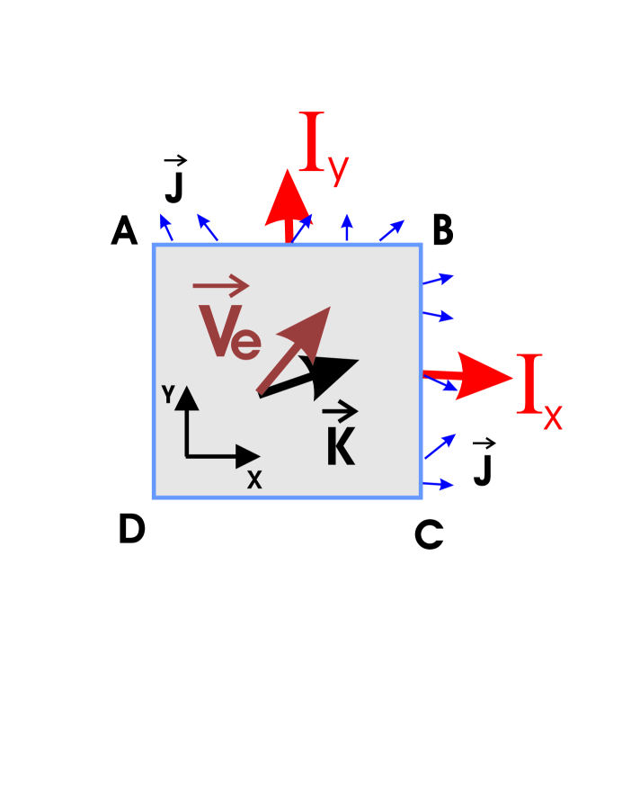
Figure 1: Conceptual layout of the EM energy flow in a unit cell.

This consideration is illustrated by Fig. 1. Here, the coordinates are shown in the figure.

According to the aforementioned equivalency theorem, the direction of the group velocity will be the direction of the spatially averaged EM energy current, i. e.

$$\langle\vec{J}\rangle=\frac{1}{S}\int_{S}d^{2}\vec{r}\vec{J}.$$ (20)

We note that the integration is performed over the whole area of the unit cell, which includes the areas occupied by the scatterers. In actual experiments, it is often difficult to probe the currents within the areas taken by the scatterers, therefore we may replace the whole integration by a partial integration

$$\langle\vec{J^{\prime}}\rangle=\frac{1}{S^{\prime}}\int_{S^{\prime}}d^{2}\vec{r}\vec{J}.$$ (21)

Here the integration is performed over the area $S^{\prime}$ which excludes the areas occupied by the scatterers.

In practice, the EM energy current through this unit cell can also be calculated from the flux across the two sides of the cell denoted by AB and BC, i. e.

$$I_{y}\sim\int_{AB}dx\vec{J}\cdot\hat{y},\ \mbox{and}\ I_{x}\sim\int_{BC}dy\vec{J}\cdot\hat{x}.$$ (22)

Here $\vec{J}$ is given by Eq. (8).

We will compare the results in Eqs (20), (21) and (22) with that obtained in Eq. (14) by the GVA:

$$I_{y}^{GVA}\sim(\nabla_{\vec{K}}\omega)\cdot\hat{y},\ \mbox{and}\ I_{x}^{GVA}\sim(\nabla_{\vec{K}}\omega)\cdot\hat{x}.$$ (23)

In the present paper, we label the averaged current in Eq. (22) as case 1, that in Eq. (20) as case 2, and that in Eq. (21) as case 3.

To simplify our discussion, we will compare the ratio between the averaged current in two directions.

• The GVA case. The angle of the group velocity is determined as

  $$\phi_{GVA}=\tan^{-1}\left(\frac{\nabla_{\vec{K}}\omega\cdot\hat{y}}{\nabla_{\vec{K}}\omega\cdot\hat{x}}\right).$$ (24)

• Case 1: $\frac{I_{y}}{I_{x}}$ from Eq. (22). we represent the ratio by the angle

  $$\phi_{1}=\tan^{-1}\left(\frac{I_{y}}{I_{x}}\right),$$ (25)

• Case 2: $\frac{\langle\vec{J}\rangle_{y}}{\langle\vec{J}\rangle_{x}}$ from Eq. (20). The corresponding angle is

  $$\phi_{2}=\tan^{-1}\left(\frac{\langle\vec{J}\rangle_{y}}{\langle\vec{J}\rangle_{x}}\right).$$ (26)

• Case 3: $\frac{\langle\vec{J}^{\prime}\rangle_{y}}{\langle\vec{J}^{\prime}\rangle_{x}}$ from Eq. (21). The corresponding angle is

  $$\phi_{3}=\tan^{-1}\left(\frac{\langle\vec{J}^{\prime}\rangle_{y}}{\langle\vec{J}^{\prime}\rangle_{x}}\right).$$ (27)

There are other options in obtain the averaged current. We refer to the setup shown in Fig. 1. If the detection is along line AB, the averaged current vector may be obtained as

$$\langle\vec{J}_{AB}\rangle=\frac{1}{L_{AB}}\int_{A}^{B}dx\vec{J}.$$ (28)

If the detection is on line BC, the averaged current vector will be

$$\langle\vec{J}_{CB}\rangle=\frac{1}{L_{CB}}\int_{C}^{B}dy\vec{J}.$$ (29)

Here $L_{AB}$ and $L_{CB}$ denote the lengths of the two sides of the unit cell. We may also consider the sum of these two averaged current if the detection is made on both AB and BC. Correspondingly, there are other three possibilities

• Case 4: $\frac{\langle\vec{J}_{CB}\rangle_{y}}{\langle\vec{J}_{CB}\rangle_{x}}$ from Eq. (29). The associated angle is

  $$\phi_{4}=\tan^{-1}\left(\frac{\langle\vec{J}_{CB}\rangle_{y}}{\langle\vec{J}_{CB}\rangle_{x}}\right).$$ (30)

• Case 5: $\frac{\langle\vec{J}_{AB}\rangle_{y}}{\langle\vec{J}_{AB}\rangle_{x}}$ from Eq. (28). The associated angle is

  $$\phi_{5}=\tan^{-1}\left(\frac{\langle\vec{J}_{AB}\rangle_{y}}{\langle\vec{J}_{AB}\rangle_{x}}\right).$$ (31)

• Case 6: $\frac{(\langle\vec{J}_{AB}\rangle+\langle\vec{J}_{CB}\rangle)_{y}}{(\langle\vec{J}_{AB}\rangle+\langle\vec{J}_{CB}\rangle)_{x}}$ from Eqs. (28) and (29). The associated angle is

  $$\phi_{6}=\tan^{-1}\left(\frac{(\langle\vec{J}_{AB}\rangle+\langle\vec{J}_{CB}\rangle)_{y}}{(\langle\vec{J}_{AB}\rangle+\langle\vec{J}_{CB}\rangle)_{x}}\right).$$ (32)

Since the energy or the current fields in the areas occupied by the scatterers, may not be easy to detect, thus there is another possibility in case 4, 5 and 6. That is, the contribution from these areas are excluded. Later we will compare the results obtained from various averageing schemes.

IV The results and discussion

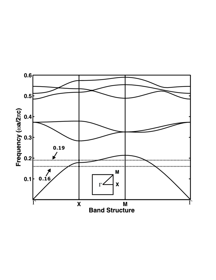
Figure 2: The band structure of a square lattice of dielectric cylinders. The lattice constant is $a$ and the radius of the cylinders is $0.3a$. $\Gamma M$ and $\Gamma X$ denote the [11] and [10] directions respectively.

The frequency band structure is plotted in Fig. 2. A complete band gap is shown between frequencies of 0.22 and 0.28. Just below the complete gap, there is a regime of partial band gap in which waves are not allowed to travel along the $\Gamma X$ or [10] direction. We will consider waves two frequencies: one is at 0.16 which is in the first passing band, and the other is at 0.19 which is within the partial bandgap.

IV.1 Two dimensional imaging of energy and energy current fields

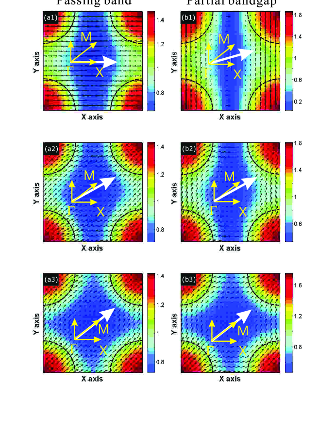
Figure 3: The imaging of the intensity fields $|\vec{E}|$ and the current of eigen-modes. Two frequencies are taken: 0.16 and 0.19 for the left and right panel respectively. (a1) $\vec{K}=(0.77\pi/a,0)$, i.e. the Bloch vector points to the angle of 0^o; (a2) $\vec{K}=(0.66\pi/a,0.38\pi/a)$, i.e. the Bloch vector points to the angle of 30^o; (a3) $\vec{K}=(0.54\pi/a,0.54\pi/a)$, i.e. the Bloch vector points to the angle of 45^o. (b1) $\vec{K}=(0.99\pi/a,0.42\pi/a)$, i.e. the Bloch vector points to the angle of 23^o; (b2) $\vec{K}=(0.87\pi/a,0.51\pi/a)$, i.e. the Bloch vector points to the angle of 30^o; (b3) $\vec{K}=(0.69\pi/a,0.69\pi/a)$, i.e. the Bloch vector points to the angle of 45^o.

First we study the spatial behavior of the energy density fields and the local flows of the eigen-modes which are characterized by the Bloch wave vectors. The current is computed by Eq. (8), while the density field is calculated by Eq. (9). The results are shown in Figure 3.

The left and right panel of Fig. 3 describes the result for frequency 0.16 and 0.19 respectively. The former lies within the first passing band, whereas 0.19 is within the first partial bandgap regime. Within this partial band, the waves are forbidden from propagation along the $\Gamma X$ direction, i.e. [10]. For each frequency, we have considered three eigen modes represented by three Bloch vectors which are given in the figure caption. The two principle directions of the unit cell, $\Gamma X$ and $\Gamma M$, are also shown in the figure.

Here we observe the following. First we discuss the case of the passing band in (a1), (a2) and (a3). Overall speaking, the flows of the energy indicated by the black arrows tend to flow along the direction indicated by the Bloch vectors. This feature is more obvious for the local current within the dielectric cylinders. For the frequency within the partial gap, however, we observe that most of the current flows may not be along the direction of the Bloch vector. Fig. 3(b1) shows that for small angles with reference to the [10] direction, all the local currents tends to flow along the direction which is close to the direction of [01]. That is, the energy flows are nearly vertical, but they cannot be exactly vertical, as the direction of [01] is a forbidden direction.

When the direction of the Bloch vector is tilted more and more away from the direction [10], an interesting feature prevails. That is, the currents eventually tends to flow into the direction of $\Gamma M$, i. e. the [11] direction. This feature is clearly demonstrated by the examples in Fig. 3(b2) and (b3) for which the Bloch vector points to the angles of 30^o and 45^o respectively.

Comparing the results for the passing band in the left panel and the results for the partial band gap in right panel of Fig. 3, we may conclude that the electromagnetic flows in periodic structures or photonic crystals will highly depend on the band structures. There are significant differences in the current behavior between the situation in which the frequency is located in a passing band and the case in which the frequency is within a partial band gap. The result shown by Fig. 3(b2) suggests that an effect of the partial band gap is to bend the current towards a direction which is to avoid the forbidden direction as much as possible; in the present case, it is the direction of $\Gamma M$ or [11]. Such feature may render possible new applications of partial band gaps in manipulating EM waves in opto-electronic devices. The results in Fig. 3 also shows that both the energy fields and the current fields are not uniform inside the unit cell. This feature indicates that the energy velocity is not also not uniform. The energy is more concentrated within the regimes occupied by the scatterers.

IV.2 Comparison of different methods obtaining the averaged currents

The results in Fig. 3 indicate that the local energy current is not uniform within a unit cell of a periodic structure. How to describe the overall energy flow in such a non-uniform situation of periodic structures thus poses an important issue.

As described in Section II.2, we mentioned that the common theoretical approach is based on the equivalence theorem between the group velocity and the averaged energy velocityYariv . The average is taken over the whole volume in three dimensions or the whole area in two dimensions, which include the volumes or the areas occupied by the scatterers. In actual experiments or observations, however, it may be difficult to probe the whole volume or the whole area to deduce the information of the averaged energy current. In particular, the currents or density within the volumes or the areas occupied by the scatterers are hard to detect. As matter of fact, there is no report on detecting the energy or energy current over the whole volume or the area to our best knowledge. The usual detection is made either at one particular spatial point or on a certain surface. In addition, it is often the intensity field that is measured.

In this section, we will compare the results obtained from the various averaging schemes outlined in Section III.2. The results will be compared with those obtained by the GVA. For brevity yet without losing generality, we consider the two frequencies from Fig. 3: 0.16 and 0.19; one is in the passing band and the other one is within the partial bandgap regime.

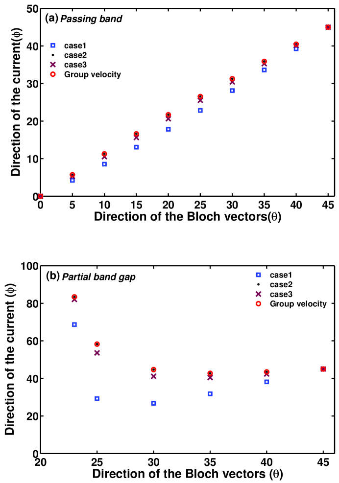
Figure 4: Comparison of four different ways obtaining the averaged EM current in a unit cell. The three cases are from Eqs. (25), (26) and (27) respectively. The results from the GVA are obtained from Eq. (24).

First, we compare the first three cases of averaging and the GVA. The three scenarios are given by Eqs. (25), (26), and (27) respectively. The results are shown in Fig. 4. Here the directions of various averaged currents and the group velocity are plotted against the direction of the Bloch wave vectors. The directions are represented by the angles of the corresponding vectors with reference to the $x$ axis.

For either the passing band or the partial bandgap cases, we see that the results from the averaging scheme 2, that is the average is taken over the whole area of the unit cell, fully agree with the results from the GVA. This verifies the equivalence theorem. It can be also seen that the results from the scheme 3 also agree reasonably well with the GVA. This implies that as long as the current inside a periodic medium can be measured, the group velocity can be well deduced by the averaging scheme, no matter whether the areas occupied by the scatterers are excluded or not. The situation is noticeably different for the averaging scheme 1, in which the information relies on the measurements along the two boundaries of the unit cell. This scheme can reproduce the results of the GVA considerably well for the passing band case in Fig. 4(a), but fails for most of the Bloch wave vectors in the partial bandgap case in Fig. 4(b). In the later case, the agreement recovers as the angle approaches 45 degree, i. e. as the direction of the Bloch vector approach that of $\Gamma M$.

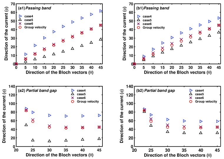
Figure 5: Comparison of the results from the averaging schemes in case 4, 5 and 6. The results in the left panel are obtained as the areas occupied by the cylinders are excluded in the average, whereas the results in the right panel are obtained when the areas are included. The three schemes are from Eqs. (31), (30) and (32) respectively. The results from the GVA are obtained from Eq. (24).

We have also compared the three other averaging schemes. The results are presented in Fig. 5. Here, we have considered both the situation in which the areas occupied by the scatterers (cylinders) are included and the case in which these areas are excluded. Here we observe the following. (1) For both the passing band and partial bandgap case, the average over any single side of the photonic crystal will either overestimate (case 4) or underestimate (case 5) the angle of the group velocity, no matter whether the areas of the cylinders are included or not. In other words, the group velocity will not represent the energy current averaged only along one observation line, as represented by the results in case 4 and 5. Relatively speaking, when the contributions from the areas of cylinders are included, the results move closer to that obtained from the GVA. (2) The results from scheme 6 are in excellent agreement with the results from the GVA, no matter whether the areas of the cylinders are included or not. This feature implies that this averaging scheme is a good candidate in inferring the group velocity of photonic crystals when the energy density and energy current inside the crystals cannot be readily probed.

Some common features can be discerned from Figs. 4 and 5. In the passing band case, the direction of the group velocity is close to that of the Bloch vector. The relation between the angles of the two is almost linear, referring to Fig. 4(a) and Fig. 5(a1) and (b1). For the first partial bandgap situation, the angle of the group velocity decreases as the angle of the Bloch vector $\vec{K}$ increases. Actually as long as the angle of the Bloch eave vector exceeds 25 degree, the angle of the group velocity saturates to the value of 45 degree. This indicates that partial gaps tend to bend currents into certain directions, allowing for possible novel applications of photonic crystals in the partial bandgap regimesChen . We have done further simulations, and found that these features are also true for other frequencies in the first passing band and first partial bandgap.

IV.3 A note on the energy density and energy flow in photonic crystals

From Fig. 3, we see that the spatial distribution of the energy density and the energy current is highly non-uniform in the unit cell. This will also indicate that the local energy velocity, defined as $\vec{v}_{e}\equiv\frac{\vec{J}_{\vec{K}}}{U_{\vec{K}}}$ with $\vec{J}_{\vec{K}}$ and $U_{\vec{K}}$ being given in Eqs. (8) and (9), is also be non-uniform. This will have some implications on the observation of the energy density and energy flows. Since the current $\vec{J}$ equals $U\vec{v}_{e}$, then with a given current magnitude, a larger local energy density (intensity) implies a smaller velocity. For instance, consider two current vectors, $\vec{J}_{1}$ and $\vec{J}_{2}$, with the same magnitude, but perpendicular to each other. Clearly, the summation of the two vectors, $\vec{J}_{T}=\vec{J}_{1}+\vec{J}_{2}$, will give a total vector which lies between the two vectors. If the magnitudes of the two corresponding current velocities are not equal, then the larger is the velocity magnitude, the smaller will be the energy density. As a result, the apparent energy density field will not be aligned along the direction of the total current $\vec{J}_{T}$. This implies that the current flow may not be readily obtainable by just measuring the energy intensity field. We may also look at this problem from another perspective. The current flow deduced from the group velocity approach, or the spatial averaged current method in case 2 and 3 say, may not be able to describe the apparent energy intensity field which is actually the quantity to be measured.

V Summary

We have considered the electromagnetic propagation in two-dimensional periodic arrays of dielectric cylinders embedded a uniform medium. The frequency band structure is computed using the standard plane-wave expansion method, and the corresponding eigne-modes are obtained subsequently. The spatially dependent optical flows of the eigen-modes are calculated by a direct computation approach. A few averaging schemes for the energy flows are discussed. The results are compared to those obtained by the common group velocity approach (GVA) which is based upon the group velocity calculation. We have considered both the case in which the frequency lies within passing band and the situation in which the frequency is in the range of a partial bandgap. It is shown that some average schemes may reproduce well the results of the GVA. With these schemes, the group velocity can be deduced in measurements. The research provides a useful information about how to obtain the group velocity and what information the traditional GVA can provide.

Appendix A Proof of $\vec{v}_{e}=\vec{v}_{g}$

For the convenience of the reader, we present a proof of $\vec{v}_{e}=\vec{v}_{g}$.

In photonic crystals, the waves assume the Bloch form,

$$\vec{E}(\vec{r})=\vec{E}_{\vec{K}}(\vec{r})e^{i\vec{K}\cdot\vec{r}},$$ (33)

and

$$\vec{H}(\vec{r})=\vec{H}_{\vec{K}}(\vec{r})e^{i\vec{K}\cdot\vec{r}},$$ (34)

where $E_{\vec{K}}$ and $\vec{H}_{\vec{K}}$ are periodic functions, and $\vec{K}$ is the Bloch wave vector.

By substituting Eqs. (33) and (34), we have

$$\vec{v}_{e}=\frac{2\mbox{Re}[\langle\vec{E}_{\vec{K}}\times\vec{H}^{\star}_{\vec{K}}\rangle]}{\langle\epsilon|\vec{E}_{\vec{K}}|^{2}+\mu|\vec{H}_{\vec{K}}|^{2}\rangle},$$ (35)

where $\langle\cdot\rangle$ denote the integration over the unit cell.

Taking eqs. (33) and (34) into the Maxwell equations (7), we have

$$\nabla\times\vec{H}_{\vec{K}}+i\vec{K}\times\vec{H}_{\vec{K}}=-i\omega\epsilon\vec{E}_{\vec{K}},$$ (36)

and

$$\nabla\times\vec{E}_{\vec{K}}+i\vec{K}\times\vec{E}_{\vec{K}}=i\omega\mu\vec{H}_{\vec{K}}.$$ (37)

Suppose now that $\vec{K}$ is changed by an infinitesimal amount, $\delta\vec{K}$. This will induce changes $\delta\omega$, $\delta\vec{E}_{\vec{K}}$, and $\delta\vec{H}_{\vec{K}}$, and they are related as

$$\nabla\times\delta\vec{H}_{\vec{K}}+i\delta\vec{K}\times\vec{H}_{\vec{K}}+i\vec{K}\times\delta\vec{H}_{\vec{K}}=-i\delta\omega\epsilon\vec{E}_{\vec{K}}-i\omega\epsilon\delta\vec{E}_{\vec{K}}$$ (38)

and

$$\nabla\times\delta\vec{E}_{\vec{K}}+i\delta\vec{K}\times\vec{E}_{\vec{K}}+i\vec{K}\times\delta\vec{E}_{\vec{K}}=i\delta\omega\mu\vec{H}_{\vec{K}}+i\omega\mu\delta\vec{H}_{\vec{K}}.$$ (39)

In the following, let us ignore the subscript $\vec{K}$.

Then we have

$$\nabla\times\vec{H}+i\vec{K}\times\vec{H}=-i\omega\epsilon\vec{E},$$ (40)

and

$$\nabla\times\vec{E}+i\vec{K}\times\vec{E}=i\omega\mu\vec{H},$$ (41)

and

$$\nabla\times\delta\vec{H}+i\delta\vec{K}\times\vec{H}+i\vec{K}\times\delta\vec{H}=-i\delta\omega\epsilon\vec{E}-i\omega\epsilon\delta\vec{E},$$ (42)

and

$$\nabla\times\delta\vec{E}+i\delta\vec{K}\times\vec{E}+i\vec{K}\times\delta\vec{E}=i\delta\omega\mu\vec{H}+i\omega\mu\delta\vec{H}.$$ (43)

Also we have

$$\nabla\times\vec{H}^{*}-i\vec{K}\times\vec{H}^{*}=i\omega\epsilon\vec{E}^{*},$$ (44)

and

$$\nabla\times\vec{E}^{*}-i\vec{K}\times\vec{E}^{*}=-i\omega\mu\vec{H}^{*}.$$ (45)

Multiplying Eq. (42) with $\vec{E}^{*}$, we get

$$\vec{E}^{*}\cdot(\nabla\times\delta\vec{H})+i\vec{E}^{*}\cdot(\delta\vec{K}\times\vec{H})+i\vec{E}^{*}\cdot(\vec{K}\times\delta\vec{H})=-i\delta\omega\epsilon|\vec{E}|^{2}-i\omega\epsilon\vec{E}^{*}\cdot\delta\vec{E},$$ (46)

and its complex conjugate is

$$\vec{E}\cdot(\nabla\times\delta\vec{H}^{*})+i\vec{E}\cdot(\delta\vec{K}\times\vec{H}^{*})+i\vec{E}\cdot(\vec{K}\times\delta\vec{H}^{*})=-i\delta\omega\epsilon|\vec{E}|^{2}-i\omega\epsilon\vec{E}\cdot\delta\vec{E}^{*},$$ (47)

Similarly, multiplying Eq. (43) with $\vec{H}^{*}$, we have

$$\vec{H}^{*}\cdot(\nabla\times\delta\vec{E})+i\vec{H}^{*}\cdot(\delta\vec{K}\times\vec{E})+i\vec{H}^{*}\cdot(\vec{K}\times\delta\vec{E})=i\delta\omega\mu|\vec{H}|^{2}+i\omega\mu\vec{H}^{*}\cdot\delta\vec{H},$$ (48)

and its complex conjugate

$$\vec{H}\cdot(\nabla\times\delta\vec{E}^{*})+i\vec{H}\cdot(\delta\vec{K}\times\vec{E}^{*})+i\vec{H}\cdot(\vec{K}\times\delta\vec{E}^{*})=i\delta\omega\mu|\vec{H}|^{2}+i\omega\mu\vec{H}\cdot\delta\vec{H}^{*},$$ (49)

Subtracting Eq. (46) from (48) and using

$$\vec{A}\cdot(\vec{B}\times\vec{C})=\vec{B}\cdot(\vec{C}\cdot\vec{A})=\vec{C}\cdot(\vec{A}\times\vec{B}),$$ (50)

we get

$$i\delta\omega(\epsilon|\vec{E}|^{2}+\mu|\vec{H}|^{2})+i\omega(\epsilon\vec{E}^{*}\cdot\delta\vec{E}+\mu\vec{H}^{*}\cdot\delta\vec{H}) = i\delta\vec{K}\cdot(\vec{E}\times\vec{H}^{*}+\vec{E}^{*}\times\vec{H})$$

$$+\vec{H}^{*}\cdot[i\vec{K}\times\delta\vec{E}+\nabla\times\delta\vec{E}]-\vec{E}^{*}\cdot[i\vec{K}\times\delta\vec{H}+\nabla\times\delta\vec{H}]$$ . (51)

The last a few terms on the RHS of Eq. (51) can be derived as

$$\vec{H}^{*}\cdot[\nabla\times\delta\vec{E}+i\vec{K}\times\delta\vec{E}]-\vec{E}^{*}\cdot[i\vec{K}\times\delta\vec{H}+\nabla\times\delta\vec{H}] = -\delta\vec{E}\cdot(i\vec{K}\times\vec{H}^{*})+\vec{H}^{*}\cdot(\nabla\times\delta\vec{E})$$

$$+\delta\vec{H}\cdot(i\vec{K}\times\vec{E}^{*})-\vec{E}^{*}\cdot(\nabla\times\delta\vec{H}).$$ (52)

Now we use

$$i\vec{K}\times\vec{H}^{*}=\nabla\times\vec{H}^{*}-i\omega\epsilon\vec{E}^{*},$$ (53)

and

$$i\vec{K}\times\vec{E}^{*}=\nabla\times\vec{E}^{*}+i\omega\mu\vec{H}^{*}.$$ (54)

Then

$$I = -\delta\vec{E}\cdot(i\vec{K}\times\vec{H}^{*})+\vec{H}^{*}\cdot(\nabla\times\delta\vec{E})+\delta\vec{H}\cdot(i\vec{K}\times\vec{E}^{*})-\vec{E}^{*}\cdot(\nabla\times\delta\vec{H})$$

$$= \ i\omega\epsilon\vec{E}^{*}\cdot\delta\vec{E}-\ \delta\vec{E}\cdot(\nabla\times\vec{H}^{*})+\vec{H}^{*}\cdot(\nabla\times\delta\vec{E})$$

$$+\ i\omega\mu\vec{H}\cdot\delta\vec{H}^{*}+\ \delta\vec{H}\cdot(\nabla\times\vec{E}^{*})-\vec{E}^{*}\cdot(\nabla\times\delta\vec{H})$$

or

$$I = i\omega\epsilon\vec{E}^{*}\cdot\delta\vec{E}+i\omega\mu\vec{H}\cdot\delta\vec{H}^{*}+\nabla\cdot(\vec{H}^{*}\times\delta\vec{E})+\nabla\cdot(\delta\vec{H}\times\vec{E}^{*}).$$ (55)

Therefore Eq. (51) becomes

$$i\delta\omega(\epsilon|\vec{E}|^{2}+\mu|\vec{H}|^{2})+i\omega(\epsilon\vec{E}^{*}\cdot\delta\vec{E}+\mu\vec{H}^{*}\cdot\delta\vec{H}) = i\delta\vec{K}\cdot(\vec{E}\times\vec{H}^{*}+\vec{E}^{*}\times\vec{H})+$$

$$i\omega\epsilon\vec{E}^{*}\cdot\delta\vec{E}+i\omega\mu\vec{H}\cdot\delta\vec{H}^{*}+$$

$$\nabla\cdot(\vec{H}^{*}\times\delta\vec{E})+\nabla\cdot(\delta\vec{H}\times\vec{E}^{*}).$$

Its complex conjugate is

$$-i\delta\omega(\epsilon|\vec{E}|^{2}+\mu|\vec{H}|^{2})-i\omega(\epsilon\vec{E}\cdot\delta\vec{E}^{*}+\mu\vec{H}\cdot\delta\vec{H}^{*}) = -i\delta\vec{K}\cdot(\vec{E}^{*}\times\vec{H}+\vec{E}\times\vec{H}^{*})+$$

$$-i\omega\epsilon\vec{E}\cdot\delta\vec{E}^{*}-i\omega\mu\vec{H}^{*}\cdot\delta\vec{H}+$$

$$\nabla\cdot(\vec{H}\times\delta\vec{E}^{*})+\nabla\cdot(\delta\vec{H}^{*}\times\vec{E}).$$

Due to the periodicity, for any periodic function $\vec{A}$ we have

$$\int dv\nabla\cdot\vec{A}=\int d\vec{S}\cdot\vec{A}=0.$$ (58)

Now we subtract Eq. (LABEL:eq:5c) from Eq. (LABEL:eq:5), then we perform the volume integration over a unit cell to get

$$2i\delta\omega\langle(\epsilon|\vec{E}|^{2}+\mu|\vec{H}|^{2})\rangle=4i\delta\vec{K}\cdot\mbox{Re}[\langle\vec{E}\times\vec{H}^{*}\rangle].$$ (59)

That is

$$\delta\omega=\vec{v}_{e}\cdot\delta\vec{K}.$$ (60)

Comparison between Eqs. (11) and (60) leads to

$$\vec{v}_{g}=\vec{v}_{e}.$$ (61)

From the above derivation, we understand the conditions for $\vec{v}_{g}=\vec{v}_{e}$ to be held are that (1) the variation $\delta\vec{K}$ can be arbitrary; (2) when the variation $\delta\vec{K}$ is small, the changes in $\omega$, $E_{K}$ and $H_{K}$ are also small.

References

- (1) E. Yablonovitch, J. Mod. Opt. 41, 173 (1994).
- (2) A. Yariv and P. Yeh, Optical waves in crystals, (John Wiley & Sons, Inc., New York, 1984).
- (3) J. Joannopoulos, R. Meade, and J. Winn, Photonic Crystals (Princeton University Press, Princeton, NJ, 1995).
- (4) F. Bloch, Z. Physik 52 (1928).
- (5) L. Brillouin, Wave Propagation in Periodic Structures: Electric Filters and Crystal Lattices, (McGraw Hill, New York, 1946; Dover Publications, New York, 1953).
- (6) L. Brillouin, Wave Propagation and Group Velocity, Leon Brillouin, (New York, Academic Press, 1960).
- (7) http://www.pbglink.com.
- (8) P. Yeh, J. Opt. Soc. Am. 69, 742 (1979).
- (9) L.-S. Chen, C.-H. Kuo, and Z. Ye, To be published in Phys. Rev. E.