Spin Relaxation in a Quantum Dot due to Nyquist Noise

Abstract

We calculate electron and nuclear spin relaxation rates in a quantum dot due to the combined action of Nyquist noise and electron-nuclei hyperfine or spin-orbit interactions. The relaxation rate is linear in the resistance of the gate circuit and, in the case of spin-orbit interaction, it depends essentially on the orientations of both the static magnetic field and the fluctuating electric field, as well as on the ratio between Rashba and Dresselhaus interaction constants. We provide numerical estimates of the relaxation rate for typical system parameters, compare our results with other, previously discussed mechanisms, and show that the Nyquist mechanism can have an appreciable effect for experimentally relevant systems.

I Introduction

The dynamics of electron and nuclear spins in quantum dots has become a focus of research recently, with part of the motivation stemming from the prospect of potential applications in the context of spintronics Wolf01 or quantum computation lossdavid ; Nielsen00 . Of particular importance are relaxation processes leading to decoherence, which have received much theoretical KhN01 ; Erlingsson02 ; Golovach03 ; AM ; Kane01 ; Wellard02 and experimental FujisawaPRB01 ; FujisawaNat02 ; HansonPRL03 ; Huettel03 ; KouwenhovenNature04 ; KrutvarNature attention within the last few years.

Relaxation between Zeeman-split spin levels involves energy dissipation, which, in quantum dots with their discrete orbital spectrum, requires coupling to external degrees of freedom (a bath). In most theoretical works, phonons have played the role of such a bath KhN01 ; Erlingsson02 ; Golovach03 . Here, we will consider the Nyquist fluctuations of electric fields produced by nearby gate electrodes as an alternative source of dissipation. Decoherence due to Nyquist noise has so far been considered extensively only for charge-based quantum computation proposals averin ; makhlin ; Dykman . The potential contribution to the spin relaxation rate of magnetic field fluctuations (due to Nyquist current noise) has been found to be very smallKhN01 . More recently, decoherence of phosphorous electron and nuclear spins in silicon due to Nyquist-noise induced fluctuations of the hyperfine constant has been analyzed in Refs. Kane01, ; Wellard02, .

In the present work, we will calculate the electron spin relaxation rate in a single lateral quantum dot (Fig. 1), due to Nyquist fluctuations of a gate voltage, combined either with electron-nuclei hyperfine interaction or spin-orbit interactions. In the case of hyperfine coupling, this also contributes to nuclear spin relaxation within the quantum dot. In the case of spin-orbit coupling, the spin relaxation rate displays a striking dependence on the directions of both the fluctuating electric field as well as the static magnetic field. The spin-orbit Nyquist mechanism considered in this work can become as efficient as coupling to piezoelectric phonons (the most important other mechanism) in realistic experimental setups. The rate grows linearly in resistance of the gate circuit.

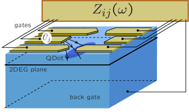
Figure 1: (Color online) Typical gated lateral quantum dot structure considered in the text, with gates connected to an electrical circuit of impedance matrix $Z$. The fluctuating electric field produced by one particular gate is shown schematically.

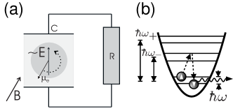
Figure 2: (a) Equivalent circuit scheme used in our model; (b) Energy diagram, showing the second-order relaxation process releasing the Zeeman energy $\hbar\omega$ into the electromagnetic environment.

In the following, we will first introduce our model Hamiltonian (Sec. II), then describe the general calculation of spin flip rates in second order Golden Rule (Sec. III), and apply this scheme to both the hyperfine (Sec. IV) and spin-orbit (Sec. V) interactions. We will comment on the relation to recent spin relaxation measurementsHuettel03 ; KouwenhovenNature04 . Finally, we will explain how the results may be applied to arbitrary gate geometries and impedances (Sec. VI) and comment on deviations due to other dot potentials or spatially inhomogeneous electric field fluctuations (Sec. VII).

II The model

We start by considering a single electron in a quantum dot formed in a 2DEG by a circularly symmetric parabolic lateral confining potential, subject to a homogeneous static magnetic field ${\mathbf{B}}$:

$$\hat{H}_{0}=\frac{\hat{\bm{\pi}}^{2}}{2m}+\frac{m\Omega_{0}^{2}}{2}{\bm{\rho}}^{2}+V(z)+\text{g}\mu_{B}{\hat{\mathbf{S}}}\cdot{\mathbf{B}},$$ (1)

where ${\hat{\bm{\pi}}}={\mathbf{\hat{p}}}-(q/c){\mathbf{A}}$ is the kinetic electron momentum, $q=-|e|$ the electron charge, ${\bm{\rho}}$ the in-plane position vector, $m$ and g the effective electron mass and g-factor respectively, $\mu_{B}>0$ the Bohr magneton, $V(z)$ the transverse confining potential, and $\Omega_{0}$ the lateral frequency.

The solutions of the in-plane orbital part are Fock-Darwin states $|n_{+}n_{-}\rangle$ with energies $n_{+}\hbar\omega_{+}+n_{-}\hbar\omega_{-}$, where $\omega_{\pm}=\sqrt{\Omega_{0}^{2}+(\omega_{c}/2)^{2}}\pm\omega_{c}/2\equiv\Omega\pm\omega_{c}/2$ and the cyclotron frequency is $\omega_{c}=|q|B_{z}/(mc)$. We will need the orbital ground state $\phi_{00}$ and the wave functions of the first excited doublet, $\phi_{00}=(\pi l)^{-1/2}\exp\left[-\rho^{2}/(2l^{2})\right]$ and $\phi_{10}=\phi_{01}^{*}=(\rho e^{i\varphi}/l)\phi_{00}$, with $x+iy=\rho e^{i\varphi}$ and $l=\sqrt{\hbar/(m\Omega)}$.

We now consider spin relaxation due to the Nyquist fluctuations of an electric field acting onto the electron, being produced by a nearby gate (see Figs. 1 and 2). We will at first assume the direction of the fluctuating field to be fixed (Fig. 2), and later describe how the analysis may be applied to arbitrary realistic gate geometries (Sec. VI). This interaction is described by

$$\hat{V}_{E}=q\hat{E}\rho_{E}=q\hat{E}(x\cos\zeta+y\sin\zeta),$$ (2)

where $\hat{E}$ is the electric field amplitude, and $\rho_{E}$ denotes the projection of the electron’s coordinate along the direction $\zeta$ of the in-plane field. We have used a dipole-approximation, assuming the electric field to be approximately constant across the dot. This purely orbital interaction can lead to spin decay only when combined with some spin-dependent part $\hat{V}_{\textrm{spin}}$ of the Hamiltonian (to be specified below). Thus, the total perturbation added to $\hat{H}_{0}$ reads:

$$\delta\hat{H}=\hat{V}_{\text{spin}}+\hat{V}_{E}.$$ (3)

Besides, the full Hamiltonian also contains a term describing the electromagnetic environment, which determines the dynamics of the electric field.

III Spin flip rate in second order Golden Rule

According to Fermi’s Golden Rule, the perturbation $\hat{V}_{E}$ produces transitions at the rate

$$\Gamma=(2\pi/\hbar^{2})\left|\langle f^{\prime}|\,\rho_{E}\,|i^{\prime}\rangle\right|^{2}e^{2}\langle\hat{E}\hat{E}\rangle_{\omega}.$$ (4)

Here $\hbar\omega=E_{i^{\prime}}-E_{f^{\prime}}$ is the energy absorbed by the environment, and $\langle\hat{E}\hat{E}\rangle_{\omega}=(2\pi)^{-1}\int dt\,e^{i\omega t}\langle\hat{E}(t)\hat{E}\rangle$ is the spectrum of the electric field. The spectrum may be related to the impedance of the gate circuit (Fig. 2) by using the Fluctuation-Dissipation Theorem (FDT) LL9 :

$$\langle\hat{E}\hat{E}\rangle_{\omega}=\pi^{-1}d^{-2}R(\omega)\hbar\omega\left(1-e^{-\hbar\omega/(k_{B}T)}\right)^{-1}.$$ (5)

Here $d$ is an effective distance determining the conversion between voltage drop and electric field (distance between capacitor plates in the simplest case; see Sec. VI for the general case). For the circuit of Fig. 2, the effective resistance responsible for the voltage fluctuations is given by $R(\omega)=R/(1+(RC\omega)^{2})$.

Spin-flip transitions are possible only because the matrix-element in Eq. (4) is to be evaluated in presence of the spin-dependent part $\hat{V}_{\textrm{spin}}$, leading to a finite admixture of different spin states. According to standard stationary perturbation theory (leading to second order Golden Rule), we have:

$$\langle f^{\prime}|\,\rho_{E}\,|i^{\prime}\rangle=\langle f\!\!\downarrow\!\!|\,\rho_{E}G(\mathcal{E}_{i\uparrow})\hat{V}_{\text{spin}}+\hat{V}_{\text{spin}}G(\mathcal{E}_{f\!\downarrow})\rho_{E}\,|i\!\!\uparrow\rangle.$$ (6)

Here, the resolvent for $\hat{H}_{0}$ is $G(\mathcal{E})=(\mathcal{E}-\hat{H}_{0})^{-1}$. For the transition between the Zeeman sublevels of the orbital ground state, we have $\mathcal{E}_{i\uparrow}=\varepsilon_{0}+\hbar\omega/2=\mathcal{E}_{f\!\downarrow}+\hbar\omega$, where $\hbar\omega=|\text{g}\mu_{B}B|$ is the Zeeman energy, and $\varepsilon_{0}$ is the energy of the orbital ground state. Eqs. (4) and (6) describe a second-order transition from $|i\!\!\uparrow\rangle$ to $|f\!\!\downarrow\rangle$. Note that $\rho_{E}$ connects the lateral orbital ground state $\phi_{00}$ to $\phi_{10}$ and $\phi_{01}$ only.

We will now consider two specific spin-flip perturbations $\hat{V}_{\textrm{spin}}$.

IV Hyperfine interaction

The hyperfine contact interaction of an electron spin $\hat{\mathbf{S}}$ with nuclear spins $\hat{\mathbf{I}}_{j}$ at positions ${\mathbf{R}}_{j}$ has the form [DPreview, ]

$$\hat{V}_{\text{HF}}={\sum}_{j}v_{0}A_{j}\,\hat{{\mathbf{S}}}\cdot\hat{{\mathbf{I}}}_{j}\;\delta({\mathbf{r}}-{\mathbf{R}}_{j}),$$ (7)

where the $A_{j}$ are the hyperfine coupling constants (depending on species), and $v_{0}$ is the volume of the unit cell. We will neglect the nuclear Zeeman splitting.

In the limit of small Zeeman splitting, $\omega\ll\Omega_{0}$, we obtain for the amplitude (6):

$$\langle f^{\prime}|\,\rho_{E}\,|i^{\prime}\rangle_{\text{HF}}=-2lv_{0}\frac{\left(1+\omega_{c}^{2}/(2\Omega_{0})^{2}\right)^{1/2}}{\hbar\Omega_{0}}{\sum}_{j}A_{j}$$

$$\times\langle\downarrow\!\!|\hat{S}^{\alpha}|\!\!\uparrow\rangle\,\langle f_{N}|\hat{I}_{j}^{\alpha}|i_{N}\rangle\Phi(z_{j},\rho_{j})\cos(\zeta-\varphi_{j}).$$ (8)

The initial and final states of the nuclear spin system are denoted $i_{N},\,f_{N}$. We have defined $\Phi(z_{j},\rho_{j})=\chi_{0}^{2}(z_{j})\phi_{00}(\rho_{j})|\phi_{10}(\rho_{j})|$, for the nuclei positions ($\rho_{j},\varphi_{j},z_{j}$), and $\chi_{0}(z)$ is the ground state of motion along the $z$-direction.

Inserting into Eq. (4) and averaging over an ensemble of unpolarized uncorrelated nuclear spins, we obtain the following expression for the electron spin relaxation rate due to Nyquist noise and hyperfine coupling:

$$\Gamma_{\text{HF}}\!=\!\frac{4\pi}{3}I(I+1)\frac{A^{2}}{(\hbar\Omega_{0})^{2}}\frac{v_{0}\eta}{z_{0}d^{2}}\frac{R(\omega)\omega}{R_{Q}}\frac{\left(1+\omega_{c}^{2}/(2\Omega_{0})^{2}\right)}{1-e^{-\hbar\omega/(k_{B}T)}},$$ (9)

where $A^{2}={\sum}_{j}A_{j}^{2}$ with summation over all nuclei in the unit cell, $R_{Q}=h/e^{2}$ is the quantum of resistance, $\eta=z_{0}l^{2}\!\int\!\Phi(z,\rho)^{2}dzd{\bm{\rho}}$ is a dimensionless form factor involving an average over nuclei positions $(z,\rho,\varphi)$, and $z_{0}$ is the 2DEG thickness.

In the following, we provide numerical estimates using typical parameters for GaAs QDs: hyperfine coupling constantMerkulov $A^{2}\simeq 1.2\times 10^{-3}$ meV², nuclear spin value $I=3/2$, unit cell volume $v_{0}=(5.65\;\text{\AA})^{3}$, effective electron mass $m=0.067m_{0}$, $|\text{g}\mu_{B}|=0.025$ meV T^-1, $\hbar\omega_{c}/B_{z}=1.76$ meV T^-1, $z_{0}=10$ nm, and a geometrical factor of $\eta=9/(16\cdot 4\pi)$ for the approximate solution of an inversion layer (triangular well) potential (see, e.g., Ref. Ando82, ).

Thus, the numerical value of the electron spin-flip rate is:

$$\Gamma_{\textrm{HF}} \approx 0.6\,\text{Hz}\times\frac{R(\omega)}{R_{Q}}\left(\frac{1\mu\text{m}}{d}\right)^{2}\left(\frac{1\text{meV}}{\hbar\Omega_{0}}\right)^{2}\frac{B}{1\text{T}}$$

$$\times\frac{1+0.8\times\left(\frac{1\,\textrm{meV}}{\hbar\Omega_{0}}\frac{B_{z}}{1\text{T}}\right)^{2}}{1-\exp\left[-0.3\times\frac{B}{1\text{T}}\frac{1\text{K}}{T}\right]}.$$ (10)

Concerning $R(\omega)=R/(1+(RC\omega)^{2})$, a lower bound for the cutoff frequency $1/(RC)$ is determined by the charging energy $E_{c}$ of the dot (involving the total capacitance $C_{\textrm{tot}}>C$), in the form $(E_{c}/\hbar)(R_{Q}/R)$. For current GaAs experiments, a typical value of $E_{c}=1$ meV yields $RC\omega\sim 10^{-1}(R/R_{Q})(B/1\text{T})$, such that $R(\omega)$ deviates from $R$ only at rather high magnetic fields, as long as $R<R_{Q}$. As a function of $R$, the maximum relaxation rate is reached at $R=1/(C\omega)$. In typical GaAs quantum dots this corresponds to $R_{\text{max}}=40R_{Q}(1\text{T}/B)$.

For a confinement frequency of $\hbar\Omega_{0}=1$ meV, the rate is equal to about $0.1\,\textrm{Hz}$ at $T=1$ K and $B=0.1$ T, with $R/R_{Q}=10^{-2}$, $d=0.5\,\mu\textrm{m}$. This is comparable to electron spin relaxation due to hyperfine interaction involving piezoelectric phonons Erlingsson02 at the same values of $\Omega_{0}$, $T$ and $B$. Since the Nyquist mechanism considered here yields a zero-temperature rate linear in transition frequency (instead of cubic as in Ref. Erlingsson02, ), it dominates at smaller magnetic fields $B<0.1\,\textrm{T}$. The relaxation rate can reach large values if the resistance approaches $R_{\text{max}}$; e.g. at $T=1$ K and $B=1$ T (with $R_{\text{max}}=40R_{Q}$), we would have $\Gamma_{\text{HF}}\simeq 0.3$ kHz, much larger than the rate due to electron-phonon coupling Erlingsson02 .

If new electrons are supplied to the dot in a transport situation or an additional electron spin relaxation mechanism is effective, then the present mechanism may also result in nuclear spin relaxation, with a rate equal to $\Gamma_{\textrm{HF}}/N$, with $N$ the number of nuclei. For the parameters used here (with $N\simeq 5\times 10^{5}$), and at $T=1$ K, $R=10^{-2}R_{Q}$, the nuclear relaxation rate turns out to be negligibly small ($10^{-7}$ Hz). In comparison, a recent transport experiment in GaAs quantum dots Huettel03 found nuclear spin relaxation times of the order of 10 minutes at $T=100$ mK and $B=40$ mT (cf. Ref. geller, for relevant theory). In order for the present Nyquist mechanism to yield a comparable rate, a resistance $R\sim R_{\textrm{max}}\sim 10^{3}R_{Q}$ would be required.

V Spin-orbit interaction

The other, numerically much more important spin-relaxation mechanism we will consider is due to the combination of Nyquist noise and spin-orbit coupling:

$$\hat{V}_{\text{SO}}=\alpha(\hat{\pi}_{x}\hat{\sigma}_{y}-\hat{\pi}_{y}\hat{\sigma}_{x})+\beta(\hat{\pi}_{y}\hat{\sigma}_{y}-\hat{\pi}_{x}\hat{\sigma}_{x}).$$ (11)

The first term in (11) is the Rashba term arising from any structural inversion asymmetry of the heterostructure, the second is the (linear) Dresselhaus term, a consequence of the bulk inversion asymmetry of the semiconductor material. The main crystallographic axes are assumed to be aligned with $x,y,z$.

By means of the commutation relations $(i\hbar/m)\hat{{\bm{\pi}}}=[{\bm{\rho}},\hat{H}_{0}]$ and $[\hat{H}_{0},\hat{{\bm{\sigma}}}]=i\text{g}\mu_{B}\hat{{\bm{\sigma}}}\times{\mathbf{B}}$, we get:

$$\hat{V}_{\textrm{SO}}=-i[{\bm{\xi}}\hat{{\bm{\sigma}}},H_{0}]+\text{g}\mu_{B}\hat{{\bm{\sigma}}}[{\mathbf{B}}\times{\bm{\xi}}],$$ (12)

where we have introduced the vector ${\bm{\xi}}=(m/\hbar)(-\beta x-\alpha y,\alpha x+\beta y,0)$.

The contribution of the first term in Eq. (12) to the amplitude, Eq. (6), yields $[\rho_{E},{\bm{\xi}}\hat{{\bm{\sigma}}}]=0$. Thus, we obtain, in the limit $\omega\ll\Omega_{0}$:

$$\langle f^{\prime}|\,\hat{\rho}_{E}\,|i^{\prime}\rangle_{\text{SO}}=\frac{\sqrt{\alpha^{2}+\beta^{2}}}{\hbar\Omega_{0}^{2}}\,\text{g}\mu_{B}\langle f\!\!\downarrow\!\!|\hat{{\bm{\sigma}}}[{\mathbf{B}}\times{\mathbf{\Omega}}]|i\!\!\uparrow\!\rangle,$$ (13)

Here, we have defined the vector ${\mathbf{\Omega}}=(\cos(\zeta-\gamma),-\sin(\zeta+\gamma),0)$, where $\gamma$ depends on the ratio of spin-orbit coupling parameters: $\tan\gamma\equiv\alpha/\beta$.

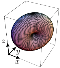
Figure 3: (Color online) Angular dependence of the spin relaxation rate $\Gamma_{\textrm{SO}}$ on magnetic field direction $(\theta,\varphi)$, according to Eq. (15), for $\varphi^{*}=-\pi/4$. The shape will be rotated around the z-axis for different values of $\varphi^{*}$, which is determined by the electric field direction $\zeta$ and the spin-orbit coupling constant ratio expressed via $\gamma$.

We parameterize the direction of the magnetic field as ${\mathbf{B}}=B(\sin\theta\cos\varphi,\sin\theta\sin\varphi,\cos\theta)$. Then the electron spin relaxation rate due to spin-orbit coupling combined with Nyquist noise is given by:

$$\Gamma_{\textrm{SO}}=4\pi\frac{\alpha^{2}+\beta^{2}}{d^{2}}\frac{R(\omega)}{R_{Q}}\,\frac{\omega^{3}}{\Omega_{0}^{4}}\,\frac{I(\zeta,\gamma\,;\theta,\varphi)}{1-e^{-\hbar\omega/(k_{B}T)}},$$ (14)

where

$$I(\zeta,\gamma;\theta,\varphi) = (\sin^{2}(\zeta+\gamma)+\cos^{2}(\zeta-\gamma))$$ (15)

$$\times\left(\cos^{2}\theta\,+\sin^{2}\theta\,\sin^{2}(\varphi-\varphi^{*})\right)$$

yields the angular dependence of the relaxation rate (see Fig. 3), with the angle $\varphi^{*}$ defined by the condition $\tan\varphi^{*}=-\sin(\zeta+\gamma)/\cos(\zeta-\gamma)$.

We note that, for fixed direction of the fluctuating electric field, $I$ vanishes for in-plane magnetic fields pointing into the direction $\varphi^{*}$, i.e. $I(\zeta,\gamma\,;\pi/2,\varphi^{*})=0,\;{\bm{\forall}}\,\zeta,\gamma$ (when ${\bm{\Omega}}\parallel\bm{B}$). In the particular case of equal spin-orbit coupling constants, $\alpha=\pm\beta$ and thus $\gamma=\pm\pi/4$, the first factor in $I$ reduces to $2\sin^{2}(\zeta\pm\pi/4)$. This means the relaxation rate may even vanish regardless of magnetic field direction, provided the electric field across the dot points along $\zeta=\mp\pi/4$, thus $I(\mp\pi/4,\pm\pi/4\,;\theta,\varphi)=0,\;{\bm{\forall}}\,\theta,\varphi$ (since ${\bm{\Omega}}=0$ in Eq. (13)). In the case of an arbitrary gate geometry (treated in Sec. VI), the rate usually does not vanish any more but can still have some pronounced directional dependence.

Conversely, for $\alpha=\pm\beta$ the rate may also vanish for arbitrary orientation $\zeta$ of the electric field, if the magnetic field lies in the plane and $\varphi=\mp\pi/4$ , i.e. $I(\zeta,\pm\pi/4\,;\pi/2,\mp\pi/4)=0,\;{\bm{\forall}}\,\zeta$. As pointed out in Ref. SchliemannPRL03, , for $\alpha=\pm\beta$ the electron spin component $\hat{\sigma}_{x}\mp\hat{\sigma}_{y}$ commutes with the spin-orbit interaction $\hat{V}_{\text{SO}}$, and for $\bm{B}\parallel(1,\mp 1,0)$ it commutes with $\hat{H}_{0}$ as well. Thus, the suppression of spin relaxation in this case is exact (see also Ref. Golovach03, ).

The numerical value for the relaxation rate is:

$$\Gamma_{\textrm{SO}}\approx 0.4\,\text{kHz}\times\frac{R(\omega)}{R_{Q}}\left(\frac{1\mu\text{m}}{d}\right)^{2}\left(\frac{1\text{meV}}{\hbar\Omega_{0}}\right)^{4}\left(\frac{B}{1\text{T}}\right)^{3}$$

$$\times\left(\frac{1\mu\textrm{m}}{\lambda_{\textrm{SO}}}\right)^{2}\,I(\zeta,\gamma\,;\theta,\varphi)\left[1-\exp\left[-0.3\times\frac{B}{1\text{T}}\frac{1\text{K}}{T}\right]\right]^{-1},$$ (16)

with $1/\lambda_{SO}^{2}\equiv(m/\hbar)^{2}(\alpha^{2}+\beta^{2})$.

The rate $\Gamma_{\textrm{SO}}$ is about $1$ Hz at $T=1$ K, for $B=0.1$ T, using the same parameters as for hyperfine interaction (and $\lambda_{\textrm{SO}}=1\mu\textrm{m}$, $I(\zeta,\gamma\,;\theta,\varphi)=1$). At these parameters, this is comparable with the relaxation rate due to the combined action of spin-orbit and piezoelectric electron-phonon interactions KhN01 ; Golovach03 , which, however, vanishes like $B^{5}$, instead of the $B^{3}$ dependence we have found here, such that the Nyquist mechanism dominates for lower fields. While a $B^{3}$-dependence was also found in Ref. KhN01, for a two-phonon relaxation process, the efficiency of that process decreases drastically when the temperature becomes lower than about $1$ K.

Very recently, the spin relaxation time in a one-electron quantum dot has been measured directly, using a time-resolved single-spin detection setupKouwenhovenNature04 . Previously, it had been possible only to obtain lower bounds on this time (see Ref. HansonPRL03, for an example). At an external magnetic field of $8{\rm T}$, the relaxation time was found to be on the order of $1{\rm msec}$. Using parameters $\hbar\Omega_{0}=1$ meV, $d=0.5\,\mu\textrm{m}$, and $\lambda_{\textrm{SO}}=1\,\mu\textrm{m}$, we indeed can obtain a rate of about $10^{4}$ Hz by assuming a reasonable value of $R/R_{Q}=10^{-2}$ (lower values of $R$ are needed if the effective $d$ is smaller). The observed magnetic field dependence is not inconsistent with a $B^{3}$ contribution, although more data are needed in this regard. Thus, the present Nyquist mechanism may be about as efficient as the piezoelectric mechanism of Ref. Golovach03, , for experimentally relevant situations, and it would be interesting to see whether the two effects can be distinguished in further measurements on similar setups (see below).

In contrast, we do not expect Nyquist noise to contribute to spin relaxation rates in self-assembled quantum dotsKrutvarNature , which are apparently well explained by piezo-electric electron-phonon couplingKhN01 alone.

As the rates $\Gamma_{\textrm{HF}}$ and $\Gamma_{\textrm{SO}}$ depend on the relevant circuit resistance $R$, it might be interesting to have a device where $R$ can be controlled (e.g. in a superconducting gate circuit, with a strong decrease in $R(\omega)$ for $T<T_{c}$ and tunability by a magnetic flux; or using varactor diodes as tunable capacitors in an $LC$-circuit). Inserting controlled dephasing by a large $R$ could be a way to cross-check measurements of spin relaxation rates (e.g. $R=4R_{Q}$ would yield an easily measurable rate $\Gamma_{SO}$ on the order of $10^{7}$Hz, for the previous parameters).

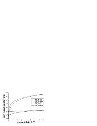
Figure 4: Electron spin relaxation rate due to Nyquist noise, Eqs. (IV) and (V), at $\hbar\Omega_{0}=1$ meV, $R/R_{Q}=10^{-2}$, $d=0.5\,\mu\textrm{m}$, $\lambda_{\textrm{SO}}=1\,\mu\textrm{m}$, $\varphi=0$, $\theta=\pi/2$, $\zeta=0$, $\gamma=-\pi/4$. At low fields, the hyperfine rate (HF) dominates over the spin orbit rate (SO).

VI Arbitrary gate geometries

We now explain how our results may be extended to arbitrary experimental configurations for gated lateral dot structures (see Fig. 1).

In general, the dot experiences a fluctuating electric field which is due to the fluctuating voltages $\hat{U}_{j}$ on the gates $j=1\ldots N_{G}$. (We assume these voltages to be measured relative to ground) The relation between the in-plane electric field components ($l=1,2$) at the center of the dot and the voltages is linear,

$$\hat{E}_{l}=\sum_{j=1}^{N_{G}}M_{lj}\hat{U}_{j}\,.$$ (17)

The real-valued matrix $M$ depends on the geometry of the gates and the dielectric substrate (it has to be obtained from an electrostatic simulation for specific geometries). This matrix has the dimension of an inverse length, and roughly corresponds to the factor $d^{-1}$ we introduced in Eq. (5) for our simple model system (which can be described by $N_{G}=2$ and $M_{l2}=-M_{l1}$ in this scheme).

The gates are nodes in an electronic circuit that is described by an impedance matrix $Z_{ij}$. Thus, according to the FDT, we have:

$$\left\langle\hat{U}_{j^{\prime}}\hat{U}_{j}\right\rangle_{\omega}=\frac{1}{2\pi}\left[Z_{j^{\prime}j}(\omega)+Z_{jj^{\prime}}^{*}(\omega)\right]\frac{\hbar\omega}{1-e^{-\hbar\omega/T}}\,.$$ (18)

We now make the reasonable assumption that the magnetic field is not strong enough to appreciably influence the impedance matrix of the circuit. Then the Onsager-Casimir relation $Z_{j^{\prime}j}(B,\omega)=Z_{jj^{\prime}}(-B,\omega)$, evaluated at $B=0$, implies reciprocity $Z_{j^{\prime}j}=Z_{jj^{\prime}}$ and thus $(Z_{j^{\prime}j}(\omega)+Z_{jj^{\prime}}^{*}(\omega))/2={\rm Re}Z_{j^{\prime}j}(\omega)$. Inserting Eq. (18) into Eq. (17), we have

$$\left\langle\hat{E}_{l^{\prime}}\hat{E}_{l}\right\rangle_{\omega}=\frac{\hbar\omega/\pi}{1-e^{-\hbar\omega/T}}\sum_{j^{\prime}j}M_{l^{\prime}j^{\prime}}M_{lj}{\rm Re}Z_{j^{\prime}j}(\omega)\,.$$ (19)

Reciprocity makes the matrix $\left\langle\hat{E}_{l^{\prime}}\hat{E}_{l}\right\rangle_{\omega}$ real-valued and symmetric. Physically, this means there is no circular component to the thermal electric field fluctuations. Thus, at given $\omega$, we can diagonalize this matrix by choosing two orthogonal directions in the 2DEG plane. The total spin relaxation rate becomes equal to the sum of the rates for these two directions, obtained according to our previous description. The angle $\zeta$ in our notation denotes the direction of the given principal axis, and $\left\langle\hat{E}\hat{E}\right\rangle_{\omega}$ is equal to the corresponding eigenvalue. As a consequence, the total spin-orbit rate $\Gamma_{SO}$ will not vanish completely for any magnetic field direction, but an anisotropy will generally remain due to the anisotropy of the gate geometry (or the impedance matrix).

However, even if the geometry were perfectly known, and the matrix $M$ were calculated using a numerical solver of the Poisson equation, it is currently difficult to go beyond estimates for realistic setups (like, e. g., those used in the experiments by the MunichHuettel03 or Delft HansonPRL03 ; KouwenhovenNature04 groups). This is because the impedance matrix of the gate circuit (and thus the noise properties) have never been studied in detail at the high frequencies under consideration, and the nominal circuit diagrams are probably valid only at low frequencies. Nevertheless, our estimate for the effective resistance entering the Nyquist noise, $R/R_{Q}\sim 10^{-2}$, seems to be roughly comparable to the actual numbers (Munich grouphuettelprivat ) or at least cannot be ruled out at present (Delft grouphansonprivat ). In this context it should also be notedhuettelprivat that part of the circuit is at higher temperatures, possibly contributing more noise than estimated using the base temperature of the setup.

VII Other dot shapes and beyond dipole approximation

If we consider an anisotropic or, in general, nonparabolic lateral confinement potential, the orbital single-particle wave functions and energies will change. Most importantly, this results in nonvanishing transition matrix elements between the ground state and more than just two excited orbital states. The same is true if we go beyond the dipole approximation, i.e. we no longer assume the fluctuating electric field to be constant across the dot.

Thus, the sum over intermediate states implicit in Eq. (6) extends over more states. However, generally speaking the qualitative picture of our previous analysis does not change, and neither do the quantiative estimates, provided the deviations from the parabolic shape are not too large. This is because transitions via higher intermediate states are suppressed anyway by larger energy denominators, and, in particular, no extra channel via low-lying energies opens up.

VIII Conclusions

In summary, we analyzed electron spin relaxation due to the combination of Nyquist noise with both hyperfine and spin-orbit interaction. For the case of spin-orbit coupling, a remarkable dependence on the directions of magnetic and electric fields is observed. For equal spin-orbit coupling constants (realizable by tuning the Rashba termSchliemannPRL03 ), the rate may vanish exactly for a particular in-plane magnetic field direction (independent of gate geometry) or, for arbitrary angles of the magnetic field, become very small provided the fluctuating electric field points predominantly into a certain fixed direction. The contribution to the spin relaxation rate may be as large as that of the most important other mechanism (piezoelectric electron-phonon coupling), for relevant experimental parameters. Furthermore, if a larger (preferably tunable) gate resistance is relevant for a given experimental setup, or microwave noise is deliberately applied to the gate, the mechanism analyzed here may dominate over an extended range of magnetic field values and might be more easily distinguished from other mechanisms.

- (1) S. A. Wolf, D. D. Awschalom, R. A. Buhrman, J. M. Daughton, S. von Molnár, M. L. Roukes, A. Y. Chtchelkanova, and D. M. Treger, Science 294, 1488 (2001).
- (2) D. Loss and D. P. DiVincenzo, Phys. Rev. A 57, 120 (1997).
- (3) M. A. Nielsen and I. L. Chuang, Quantum Computation and Quantum Information (Cambridge University Press, Cambridge, New York, 2000).
- (4) A.V. Khaetskii and Y.V. Nazarov, Phys. Rev. B 64, 125316 (2001).
- (5) S. I. Erlingsson and Y. V. Nazarov, Phys. Rev. B 66, 155327 (2002).
- (6) V. N. Golovach, A. Khaetskii, and D. Loss, Phys. Rev. Lett. 93, 016601 (2004).
- (7) V. A. Abalmassov and F. Marquardt, Phys. Rev. B 70, 075313 (2004).
- (8) B. E. Kane, Fortschritte der Physik 48, 1023 (2001).
- (9) C. J. Wellard and L. C. L. Hollenberg, J. Phys. D: Appl. Phys. 35, 2499 (2002).
- (10) T. Fujisawa, Y. Tokura, and Y. Hirayama, Phys. Rev. B 63, 081304(R) (2001).
- (11) T. Fujisawa, D. G. Austing, Y. Tokura, Y. Hirayama, and S. Tarucha, Nature (London) 419, 278 (2002).
- (12) R. Hanson, B. Witkamp, L. M. K. Vandersypen, L. H. Willems van Beveren, J. M. Elzerman, and L. P. Kouwenhoven, Phys. Rev. Lett. 91, 196802 (2003).
- (13) A. K. Hüttel, J. Weber, A. W. Holleitner, D. Weinmann, K. Eberl, and R. H. Blick, Phys. Rev. B 69, 073302 (2004).
- (14) J. M. Elzerman, R. Hanson, L. H. W. van Beveren, B. Witkamp, L. M. K. Vandersypen, and L. P. Kouwenhoven, Nature 430, 431 (2004).
- (15) M. Kroutvar et al., Nature 432, 81 (2004).
- (16) D. V. Averin, Solid State Communications 105, 659 (1998).
- (17) Yu. Makhlin, G. Schön, and A. Shnirman, Rev. Mod. Phys. 73, 357-400 (2001).
- (18) M. I. Dykman, P. M. Platzman, and P. Seddighrad, Phys. Rev. B 67, 155402 (2003).
- (19) L. D. Landau and E. M. Lifshitz, Statistical Physics, Part 2 (Pergamon Press Ltd 1980).
- (20) M.I. Dyakonov and V.I. Perel, in Optical Orientation, edited by F. Meier and B.P. Zakharchenya (Elsevier, Amsterdam, 1984).
- (21) I. A. Merkulov, Al. L. Efros, and M. Rosen, Phys. Rev. B 65, 205309 (2002).
- (22) T. Ando, A. B. Fowler, and F. Stern, Rev. Mod. Phys. 54, 437 (1982).
- (23) Y. B. Lyanda-Geller, I. L. Aleiner, and B. L. Altshuler, Phys. Rev. Lett. 89, 107602 (2002).
- (24) J. Schliemann, J. C. Egues, and D. Loss, Phys. Rev. Lett. 90, 146801 (2003).
- (25) A. K. Hüttel, priv. commun.
- (26) R. Hanson, priv. commun.