Interference effect in the Landau-Zener tunneling of the antiferromagnetically coupled dimer of single-molecule magnets

Abstract

Two antiferromagnetically coupled tunneling systems is a minimal model exhibiting the effect of quantum-mechanical phase in the Landau-Zener effect. It is shown that the averaged staying probability oscillates vs resonance shift between the two particles, as well as vs sweeping rate. Such a resonance shift can be produced in Mn₄ dimers by the gradient of the magnetic field.

Tunneling at an avoided level crossing, or the Landau-Zener (LZ) effect lan32 ; zen32 is a quantum phenomenon that was much studied in physics of atomic and molecular collisions. Recently an experimental technique using the LZ effect was applied to single-molecule magnets to extract their tunneling level splitting $\Delta$.werses99 ; weretal00epl

In spite of the quantum nature of the LZ effect, its basic form can be described classically by a Landau-Lifshitz equation for a magnetic moment in a time-dependent field.chugar02 ; gar03prb ; garsch04prb However different kinds of interactions between tunneling magnetic molecules in a crystal make the LZ effect much more complicated. If the interactions are treated within the mean-field approximation (MFA), then the LZ tunneling can still be described by a nonlinear Schrödinger equation or, equivalently, by a classical nonlinear Landau-Lifshitz equation. In general, one is left with a tremendous problem of solving a full Schrödinger equation for an $N$-particle system.

The question of how good is the MFA for the LZ effect with interaction was studied in detail for the idealized “spin bag” model of $N$ tunneling particles interacting each with each with the same coupling strength $J$. gar03prb ; garsch04prb This model can be mapped onto the problem of the giant spin $S=N/2,$ so that the MFA limit $N\rightarrow\infty$ corresponds to the classical limit $S\rightarrow\infty.$ In Ref. garsch04prb, it was shown that if the classical trajectory is smooth, the MFA yields qualitatively correct results, and quantum corrections can be calculated with the help of the cumulant expansion. In the case of complicated classical motion the MFA becomes unreliable.

For the spin-bag model, both the MFA and the full quantum-mechanical solutions show that the ferromagnetic coupling suppresses LZ transitions (i.e., increases the LZ staying probability $P$), whereas the antiferromagnetic (AF) coupling increases transitions. This is in accord with physical expectations based on the time dependence of the total field on a magnetic molecule, the sum of the external sweep field and the molecular field from the neighboring molecules. If one of the molecules tunnels, then for the ferromagnetic coupling the jump of the total field is positive, so that the neigboring molecules are being brought past the resonance and lose their chance to tunnel. For the AF-coupling, the jump of the total field is negative, so that the neigboring molecules recieve an additional chance to tunnel and thus $P$ decreases.

A more realistic model for the LZ effect with interaction should incorporate both distance-dependent couplings and individual resonance fields for magnetic molecules. Recently obtained solution for this model in the fast-sweep limit garsch03prl showed an oscillating dependence of the averaged one-particle staying probability $P_{\mathrm{avr}}$ of the system on the resonance shifts between the molecules on the $i$th and $j$th lattice sites. This is an essentially quantum-mechanical effect arising due to the possibility to reach the same final state by different sequences of individual tunneling events. The different quantum-mechanical phases accumulated on different ways lead to the interference in the final state. This poses a major challenge in the theoretical description of macroscopic systems since the phase factors are very sensitive to the microscopic details and dephasing processes should play a big role. Certainly the effect of interfering tunneling paths cannot be described by the MFA.

\begin{picture}(11.0,6.5)\centerline{\hbox{\psfig{angle=-90,width=284.52756pt}}} \end{picture}

Figure 1: Bare energy levels for two antiferromagnetically coupled tunneling systems for $V<4J$.

The minimal model that exhibits the phase effect in the LZ tunneling is the model of two antiferromagnetically coupled tunneling systems (see Fig. 1) that describes a particular transition in the recently discovered Mn-4 dimer. weralihenchr02nature ; hiledwalichr03science We will use the Hamiltonian

$$\widehat{H}=-\frac{1}{2}\sum_{i=1}^{2}\left\{\left[W(t)-V_{i}\right]\sigma_{iz}+\Delta\sigma_{ix}\right\}+J\sigma_{1z}\sigma_{2z},$$ (1)

where $\mathbf{\sigma}_{i}$ are Pauli matrices, $W(t)=vt\$is the global time-linear energy sweep, $\Delta$ is the level splitting, $J$ is the coupling, and we set

$$V_{1}=-V/2,\qquad V_{2}=V/2,$$

so that $V=V_{2}-V_{1}$ is the resonance shift. For $V>0$ particle 1 crosses the resonance first. The bare energy eigenvalues for this Hamiltonian are

$$E_{-,-} = W(t)+J,\qquad E_{+,+}=-W(t)+J$$

$$E_{+,-} = -V/2-J,\qquad E_{-,+}=V/2-J,$$ (2)

where $+,-$ means spin 1 up and spin 2 down. There are four first-order level crossings:

$$E_{-,-} = E_{+,-}\quad\Rightarrow\quad W(t)=-V/2-2J=W_{1}$$

$$E_{-,-} = E_{-,+}\quad\Rightarrow\quad W(t)=V/2-2J=W_{2}$$

$$E_{-,+} = E_{+,+}\quad\Rightarrow\quad W(t)=-V/2+2J=W_{3}$$

$$E_{+,-} = E_{+,+}\quad\Rightarrow\quad W(t)=V/2+2J=W_{4}.$$ (3)

The central crossing, $E_{-,-}=E_{+,+}\quad\Rightarrow\quad W=0$ is the second-order crossing with the splitting $\sim\Delta^{2}/J$ that can be neglected in the case of well-separated resonances.gar03prb In this case one has four independent LZ transitions, each described by a scattering matrix (see, e.g., Ref. kay93, )

$$M=\left(\begin{array}[]{cc}\sqrt{P}&\sqrt{1-P}e^{-i\phi}\\ -\sqrt{1-P}e^{i\phi}&\sqrt{P}\end{array}\right),$$ (4)

where

$$P=e^{-\varepsilon},\qquad\varepsilon=\frac{\pi\Delta^{2}}{2\hbar v}$$ (5)

is the Landau-Zener staying probability and

$$\phi=\pi/4+\mathrm{Arg}\Gamma\left(1-i\delta\right)+\delta\left(\ln\delta-1\right)$$ (6)

with $\delta\equiv\varepsilon/(2\pi).$ Evolution of the wave function between level crossings reduces to the accumulation of the phase factors $\exp\left[i\Phi_{\alpha\beta}(t)\right],$ where the phases

$$\Phi_{\alpha\beta}(t)=-\frac{1}{\hbar}\int^{t}dt^{\prime}E_{\alpha\beta}(t^{\prime}),\qquad\alpha,\beta=\pm$$ (7)

can be easily calculated for the linear sweep from Eq. (2) and are quadratic in $W.$ The wave function of the system can be written as $\Psi(t)=\sum_{\alpha\beta}C_{\alpha\beta}(t)\left|\alpha\beta\right\rangle.$ Before the first crossing one has both spins down, $C_{-,-}=1$ (dropping an irrelevant phase factor) and $C_{\alpha\beta}=0$ otherwise. We use thus defined wave function $C_{\alpha\beta}^{\mathrm{in}}$ as the initial condition and we introduce

$$\Delta\Phi_{\alpha\beta}\left(W_{2},W_{1}\right)\equiv\Phi_{\alpha\beta}\left(W_{2}\right)-\Phi_{\alpha\beta}\left(W_{1}\right).$$ (8)

Then after the fourth crossing one has

$$C_{\alpha^{\prime\prime}\beta^{\prime\prime}}^{\mathrm{out}} = \left(\delta_{\alpha^{\prime\prime},+}M_{\beta^{\prime\prime}\beta^{\prime}}+\delta_{\alpha^{\prime\prime},-}\delta_{\beta^{\prime\prime}\beta^{\prime}}\right)$$ (9)

$$\times e^{i\Delta\Phi_{\alpha^{\prime\prime}\beta^{\prime}}\left(W_{4},W_{3}\right)}\left(\delta_{\beta^{\prime},+}M_{\alpha^{\prime\prime}\alpha^{\prime}}+\delta_{\beta^{\prime},-}\delta_{\alpha^{\prime\prime}\alpha^{\prime}}\right)$$

$$\times e^{i\Delta\Phi_{\alpha^{\prime}\beta^{\prime}}\left(W_{3},W_{2}\right)}\left(\delta_{\alpha^{\prime},-}M_{\beta^{\prime}\beta}+\delta_{\alpha^{\prime},+}\delta_{\beta^{\prime}\beta}\right)$$

$$\times e^{i\Delta\Phi_{\alpha^{\prime}\beta}\left(W_{2},W_{1}\right)}M_{\alpha^{\prime}\alpha}C_{\alpha\beta}^{\mathrm{in}},$$

that is the final state. In this formula summation over repeated indices is implied. The staying probability for the first and second particles are given by

$$P_{1} = 1-\left|c_{+,-}\right|^{2}-\left|c_{+,+}\right|^{2}$$

$$P_{2} = 1-\left|c_{-,+}\right|^{2}-\left|c_{+,+}\right|^{2}.$$ (10)

The average one-particle staying probability and the reduced magnetization read

$$P_{\mathrm{avr}} = \frac{1}{2}\left(P_{1}+P_{2}\right)=1-\frac{1}{2}\left|c_{+,-}\right|^{2}-\frac{1}{2}\left|c_{-,+}\right|^{2}-\left|c_{+,+}\right|^{2}$$

$$M = 1-2P_{\mathrm{avr}}.$$ (11)

After some algebra one obtains from Eq. (9) the results

$$P_{1}=P^{2}(2-P)$$ (12)

$$P_{2}=P(2-P)(1-P+P^{2})-2P(1-P)^{2}\cos\left[\frac{4JV}{\hbar v}\right]$$

and

$$P_{\mathrm{avr}}=P\left(1-\frac{P}{2}\right)(1+P^{2})-P(1-P)^{2}\cos\left[\frac{4JV}{\hbar v}\right],$$ (13)

where the argument of the cos can be rewritten as

$$\frac{4JV}{\hbar v}=\frac{8JV}{\pi\Delta^{2}}\varepsilon.$$ (14)

This is exactly the phase argument in Eq. (8) of Ref. garsch03prl, . The oscillating quantum-phase term in our solution arises because the state $\left|\downarrow\downarrow\right\rangle$ can be reached in two different ways: (i) Spin 1 flips first and spin 2 flips second (crossings at $W=W_{1}$ and $W_{4});$ (ii) Spin 2 flips first and spin 1 flips second (crossings at $W=W_{2}$  and $W_{3}).$ The amplitudes of these two processes add up, and the accumulated phase difference leads to oscillations.

The interference effect in a system of two tunneling particles takes place for the AF coupling only. For the ferromagnetic coupling, the two horizontal lines corresponding to $\left|\uparrow\downarrow\right\rangle$ and $\left|\downarrow\uparrow\right\rangle$ go above the (inactive) cental crossing, cf. Fig. 1. As a result, there are only transitions at crossings at $W_{1}$ and $W_{2}$ [see Eqs. (3)] but no transitions at $W_{3}$ and $W_{4}.$ Instead of Eq. (9) one has

$$c_{\alpha^{\prime}\beta^{\prime}}^{\mathrm{out}}=\left(\delta_{\alpha^{\prime},-}M_{\beta^{\prime}\beta}+\delta_{\alpha^{\prime},+}\delta_{\beta^{\prime}\beta}\right)e^{i\Delta\Phi_{\alpha^{\prime}\beta}\left(W_{2},W_{1}\right)}M_{\alpha^{\prime}\alpha}c_{\alpha\beta}^{\mathrm{in}},$$ (15)

and the results for the probabilities are

$$P_{1} = P,\qquad P_{2}=1-P+P^{2}$$

$$P_{\mathrm{avr}} = (1+P^{2})/2.$$ (16)

Note that $P_{\mathrm{avr}}$ coincides with Eq. (20) of Ref. gar03prb, for $N=2$ and is independent on the resonance shift. In this model $P_{\mathrm{avr}}\geq 1/2$ because tunneling of both particles is impossible, $C_{+,+}=0.$ The case of a strong resonance shift corresponds to $V>4|J|.$ In this case the coupling plays no role, and one obtains $P_{1}=P_{2}=P.$

Let us now consider the fast-sweep limit, $\varepsilon\ll 1.$ In this case one can write the expansion of the averaged staying probability in the form

$$P_{\mathrm{avr}}\cong 1-\varepsilon+\varepsilon^{2}/2+\varepsilon^{2}I_{0},$$ (17)

where $I_{0}$ describes the deviation from the standard LZ effect, Eq. (5), due to the interaction. garsch03prl For not too large resonance shifts, $V<4|J|,$ one obtains from Eqs. (13) and (16)

$$I_{0}=\left\{\begin{array}[]{ll}-1/2-\cos\left(\frac{8JV}{\pi\Delta^{2}}\varepsilon\right),&J>0\\ 1/2,&J<0\end{array}\right.$$ (18)

that is equivalent to Eq. (18) of Ref. garsch03prl, . For large couplings and resonance shifts, the cos-term in Eq. (18) oscillates fast and averages out. In this case one can conclude that the effects of antiferro- and ferromagnetic couplings are just the opposite: The former enhances transitions while the latter suppresses transitions by the same amount.

Our present model allows, however, to analyze the influence of interactions in the whole range of sweep rates, and it shows that the effect of the AF coupling is smaller than that of the ferromagnetic coupling. Dropping the cos-term in Eq. (13), one obtains

$$\overline{P}_{\mathrm{avr}}-P=\left\{\begin{array}[]{ll}-P^{2}\left(1-P\right)^{2}/2,&J>0\\ \left(1-P\right)^{2}/2,&J<0.\end{array}\right.$$ (19)

For $J>0$ this difference is small everywhere, and its absolute value attains a maximum at $P=1/2,$ where $\overline{P}_{\mathrm{avr}}-P=-1/32.$ On the other hand, for the ferromagnetic coupling $\overline{P}_{\mathrm{avr}}-P$  tends to 1/2 in the slow-sweep limit, $\varepsilon\gg 1.$

\begin{picture}(11.0,6.5)\centerline{\hbox{\psfig{angle=-90,width=256.0748pt}}} \end{picture}

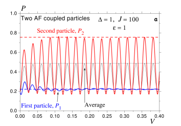
\begin{picture}(11.0,6.0)\centerline{\hbox{\psfig{angle=-90,width=256.0748pt}}} \end{picture}

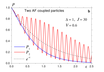
Figure 2: Staying probabilities for a system of two antiferromagnetically coupled particles $a$ – vs. resonanse shift $V$. Asymptotic values are shown by horizontal dased lines. $b$ – vs sweep parameter $\varepsilon$.

Numerical solution of the LZ problem for two AF-coupled tunneling systems is shown in Fig. 2. One can see from Fig. 2$a$ that for $J\gg\Delta$ the staying probabilities $P_{2}$ and $P_{\mathrm{avr}}$ begin to oscillate starting from the values of the resonance shift $V$ that satisfy $V\ll\Delta.$ The numerical data for $P_{\mathrm{avr}}$  is well described by Eq. (13) starting from $V\approx 0.1.$ On the other hand, for $P_{1}$ and $P_{2}$ the condition of well-separated resonances is more restrictive and it requires somewhat greater values of $V$ to validate Eqs. (12). Fig. 2$b$ shows oscillations of $P_{2}$ as a function of the sweep parameter $\varepsilon,$ as well as a faster decay of $P_{1}$ in comparison to the standard LZ effect.

Let us now discuss the application of the present results to Mn₄ dimers. The coupling between the two Mn₄ monomers with $S=9/2$ was shown to have the form of the isotropic exchange, tirwerfogalichr03prl $\widehat{H}_{\mathrm{ex}}=J_{\mathrm{ex}}\mathbf{S}_{1}\cdot\mathbf{S}_{2}$ with $J_{\mathrm{ex}}\simeq 0.1$ K for the mostly studied compound.weralihenchr02nature ; hiledwalichr03science Density-functional theory calculationsparketal03prb yield somewhat larger values of $J_{\mathrm{ex}}.$ The uniaxial anisotropy $D\simeq 0.75$ K creates a barrier for spin tunneling. The level splitting between the ground states $\left|\pm 9/2\right\rangle$ in the Mn₄ monomer is $\Delta\simeq$ 2$\times 10^{-7}$ K (Ref. werbhaboschrhen03prbrc, ) and it should be of the same order of magnitude in the Mn₄ dimer. The ground-state tunneling in a Mn₄ dimer can be described by a pseudospin Hamiltonian of Eq. (1) with $J=S^{2}J_{\mathrm{ex}}\simeq 2$ K. The period of oscillations on the resonance shift $V$ follows from Eqs. (13) and (14) and is given by $V_{\mathrm{Period}}=\left(\pi^{2}/4\right)\Delta^{2}/(J\varepsilon).$ For $\varepsilon=1$ one obtains $V_{\mathrm{Period}}\simeq 5\times 10^{-14}$ K that corresponds to the difference of longitudinal magnetic fields $\Delta H\simeq 10^{-14}$ T between the two monomers. With the distance between the monomers $l\simeq 10$ Å, this amounts to the very small field gradient, $dH/dx\simeq 10^{-3}$ Gauss/cm! This means that small inhomogeneities of the magnetic field, due to, e.g., dipole-dipole interaction, should average out the quantum oscillations in the LZ effect. For possible applications in quantum computing, it is desirable to have a larger tunnel splitting $\Delta,$ to achieve a faster performance rate and reduce the influence of decoherence. This can be achieved by applying a transverse magnetic field. In this case the period of the quantum oscillations considered here will be much larger, and their observation will require much robuster field gradients that will exceed uncontrolled inhomogeneities of the magnetic field.

The author thanks R. Schilling for many stimulating discussions.

References

- (1) L. D. Landau, Phys. Z. Sowjetunion 2, 46 (1932).
- (2) C. Zener, Proc. R. Soc. London A 137, 696 (1932).
- (3) W. Wernsdorfer and R. Sessoli, Science 284, 133 (1999).
- (4) W. Wernsdorfer, R. Sessoli, A. Caneshi, D. Gatteschi, and A. Cornia, Europhys. Lett. 50, 552 (2000).
- (5) E. M. Chudnovsky and D. A. Garanin, Phys. Rev. Lett. 89, 157201 (2002).
- (6) D. A. Garanin, Phys. Rev. B 68, 014414 (2003).
- (7) D. A. Garanin and R. Schilling, Phys. Rev. B 69, 104412 (2004).
- (8) D. A. Garanin and R. Schilling, (cond-mat/0312030).
- (9) W. Wernsdorfer, N. Aliaga-Alcalde, D. N. Hendrickson, and G. Christou, Nature 416, 406 (2002).
- (10) S. Hill, R. S. Edwards, N. Aliaga-Alcalde, and G. Christou, Science 302, 1015 (2003).
- (11) Y. Kayanuma, Phys. Rev. B 47, 9940 (1993).
- (12) R. Tiron, W. Wernsdorfer, D. Foguet-Albiol, N. Aliaga-Alcalde, and G. Christou, Phys. Rev. Lett. 91, 227203 (2003).
- (13) Kyungwha Park, M. R. Pederson, S. L. Richardson, N. Aliaga-Alcalde, and G. Christou, Phys. Rev. B 68, 020405 (2003).
- (14) W. Wernsdorfer, S. Bhaduri, C. Boskovic, G. Christou, and D. N. Hendrickson, Phys. Rev. B 68, 140407 (2003).