Orbital and spin interplay in spin-gap formation in pyroxene $A$TiSi₂O₆ ($A$=Na, Li)

Abstract

Interplay between orbital and spin degrees of freedom is theoretically studied for the phase transition to the spin-singlet state with lattice dimerization in pyroxene titanium oxides $A$TiSi₂O₆ ($A$=Na, Li). For the quasi one-dimensional spin-$1/2$ systems, we derive an effective spin-orbital-lattice coupled model in the strong correlation limit with explicitly taking account of the $t_{2g}$ orbital degeneracy, and investigate the model by numerical simulation as well as the mean-field analysis. We find a nontrivial feedback effect between orbital and spin degrees of freedom; as temperature decreases, development of antiferromagnetic spin correlations changes the sign of orbital correlations from antiferro to ferro type, and finally the ferro-type orbital correlations induce the dimerization and the spin-singlet formation. As a result of this interplay, the system undergoes a finite-temperature transition to the spin-dimer and orbital-ferro ordered phase concomitant with the Jahn-Teller lattice distortion. The numerical results for the magnetic susceptibility show a deviation from the Curie-Weiss behavior, and well reproduce the experimental data. The results reveal that the Jahn-Teller energy scale is considerably small and the orbital and spin exchange interactions play a decisive role in the pyroxene titanium oxides.

I Introduction

Orbital degree of freedom has attracted much attention since it plays key roles in electronic properties of transition metal compounds.Tokura2000 ; Imada1998 The orbital degree of freedom couples with the Jahn-Teller (JT) lattice distortion, and in many compounds, the energy scale of the JT stabilization energy is larger than that of the spin and orbital exchange interactions.Kugel1982 A typical example is the mother compound of colossal magnetoresistive (CMR) manganites, LaMnO₃: The JT energy scale is $\sim 0.1$-$1$eV and the spin exchange energy scale is $\sim 10$meV. Consequently, the orbital-lattice transition occurs at a much higher temperature ($\sim 800$K) than the antiferromagnetic (AF) transition temperature ($\sim 140$K).Wollan1955 In these systems, the orbital-lattice physics is dominant, and the orbital and lattice orderings modify effective spin exchange interactions to lead a magnetic ordering in a secondary effect. Moreover, the JT distortion suppresses fluctuation effects in orbital and spin degrees of freedom. Hence, a large JT coupling masks bare interplay between spin and orbital in many real materials.

Quantum and thermal fluctuations in the competition between the spin and orbital exchange interactions may yield novel phenomena, and therefore, it is highly desired to explore systems in which the genuine spin-orbital interplay appears explicitly. One of promising candidates is the $t_{2g}$ electron system such as titanium and vanadium oxides. In the $t_{2g}$ systems, the JT coupling becomes smaller than in the $e_{g}$ systems such as CMR manganites because spatial shapes of $t_{2g}$ orbitals avoid directions of surrounding ligands in the octahedral positions. For instance, in vanadium perovskite oxides $A$VO₃ ($A$=La, Ce), the orbital-lattice transition temperature becomes even lower than the AF one,Miyasaka2003 and novel interplay between spin and orbital is proposed theoretically.Motome2003 ; Khaliullin2001

Figure 1: (a) Lattice structure of pyroxene oxides $A$TiSi₂O₆ ($A$=Na, Li). Chains of TiO₆ octahedra are separated by SiO₄ tetrahedra. (b) Skew edge-sharing chain structure of TiO₆ octahedra. Balls in the center of each octahedron denote Ti cations, and oxygen ions are on the corners of the octahedra. The octahedra share their edges in the $xy$ and $yz$ planes alternatively. White objects with four lobes denote $d_{xy}$ and $d_{yz}$ orbitals of $t_{2g}$ electrons, and $t^{11}$ ($t^{22}$) is the $\sigma$-bond transfer integrals between $d_{xy}$ ($d_{yz}$) orbitals. See the text for details.

Pyroxene titanium oxides $A$TiSi₂O₆ ($A$=Na, Li) are typical examples of the $t_{2g}$ electron systems where such interplay between spin and orbital is expected.Isobe2002 The lattice structure of these compounds consists of characteristic one-dimensional (1D) chains of skew edge-sharing TiO₆ octahedra as shown in Fig. 1 (a). The TiO₆ chains are bridged and well separated by SiO₄ tetrahedra, and therefore, interchain couplings are considered to be much weaker than intrachain interactions. In each TiO₆ chain, as shown in Fig. 1 (b), the edges of octahedra in the $xy$ and $yz$ planes are alternatively shared between neighboring octahedra, which leads to the zig-zag structure. Each magnetic Ti³⁺ cation has one $d$ electron in these insulating materials. Hence, we may consider that a quasi 1D spin-$1/2$ system is realized.

Pyroxene titanium oxides show a peculiar phase transition. The magnetic susceptibility shows a sharp drop at $T_{\rm c}=210$K and $230$K in NaTiSi₂O₆ and LiTiSi₂O₆, respectively, which indicates the transition to a spin-singlet state with a finite spin gap.Isobe2002 Below $T_{\rm c}$, a dimerization of Ti-Ti distances along the chain was observed by the X-ray scattering.Ninomiya2003 These remind us of a spin-Peierls transition.Boucher1996 However, above $T_{\rm c}$, the magnetic susceptibility shows an unusual temperature dependence which clearly deviates from that of other spin-Peierls compounds. In spin-Peierls systems, the dimerization is caused by the magnetoelastic coupling, and therefore, the transition occurs when short-range spin correlations develop enough to drive the lattice dimerization. This development of spin correlations is manifested in a broad peak of the magnetic susceptibility above $T_{\rm c}$, and the peak temperature gives a rough estimate of the spin exchange energy scale. Contrary to this conventional behavior, the magnetic susceptibility of the pyroxene compounds at high temperatures increases as temperature decreases, and suddenly drops at $T_{\rm c}$ without a clear formation of the broad peak.Isobe2002 This suggests a breakdown of the simple spin-Peierls picture in these pyroxene compounds.

For the peculiar transition to the spin-singlet state, an importance of the $t_{2g}$ orbital degree of freedom has been pointed out. Isobe2002 Theoretically, a scenario of the orbital-driven spin-singlet formation has been explored in spin-orbital coupled models for $t_{2g}$ electron systems. Katoh1999 It was proposed that the orbital ordering may modify effective spin exchange interactions and induce the spin-singlet formation. However, models were considered only for systems with corner-sharing octahedra, and hence, it is unclear that the argument is applicable to the present pyroxene systems with the edge-sharing octahedra. A similar scenario has been proposed for the present systems,Konstantinovic2004 however, the analysis was heuristic and not sufficient to conclude the mechanism of the finite-temperature transition. In order to clarify the nature of the transition and the low-temperature phase, we need more elaborate analysis. In particular, it is indispensable to investigate thermodynamic properties on the basis of a microscopic model.

In the present study, we will theoretically explore the mechanism of the unusual phase transition in the pyroxene titanium oxides $A$TiSi₂O₆ explicitly taking account of the $t_{2g}$ orbital degree of freedom. We derive an effective spin-orbital-lattice coupled model in the strong correlation limit, and investigate thermodynamics as well as the ground-state properties of the model applying the numerical quantum transfer matrix method and mean-field-type arguments. As a result, we find that interesting interplay between orbital and spin degrees of freedom occurs in the system, and the interplay gives a comprehensive understanding of the peculiar properties of the pyroxene compounds: Although both orbital and spin correlations are antiferro type and compete with each other at high temperatures, development of AF spin correlations with decreasing temperature yields a sign change of orbital correlations from antiferro to ferro type. After the sign change, the ferro-type orbital correlations grow with the antiferro-type spin correlations, and finally, induce the spin-singlet formation with a dimerization. Furthermore, the nontrivial temperature dependence of orbital correlations modifies an effective magnetic coupling, and results in a non Curie-Weiss behavior of the magnetic susceptibility. We show that our model with realistic parameters reproduces the peculiar temperature dependence of the magnetic susceptibility in experiment.

The organization of this paper is as follows. In the following section II, applying the strong-coupling approach, we derive an effective spin-orbital-lattice coupled model for the $t_{2g}$ pyroxene compounds $A$TiSi₂O₆. In Sec. III, we discuss properties of the system in the ground state and in the high-temperature limit using mean-field type arguments. In Sec. IV, we study thermodynamic properties of the effective model by numerical simulations. We describe the method in Sec. IV.1. Section IV.2 shows the numerical results including quantitative comparisons with the experimental data. Finally, Section V is devoted to summary and concluding remarks.

II Model Hamiltonian

In this section, we derive an effective spin-orbital-lattice coupled model for the pyroxene oxides $A$TiSi₂O₆, whose Hamiltonian reads

$$\mathcal{H}=\mathcal{H}_{\rm so}+\mathcal{H}_{\rm JT}+\mathcal{H}_{\perp}.$$ (1)

The first term describes the intersite exchange interactions in spin and orbital degrees of freedom, and the second term includes the Jahn-Teller type orbital-lattice coupling. These two are defined within each 1D chain. The third term describes the interchain coupling.

The spin-orbital exchange Hamiltonian $\mathcal{H}_{\rm so}$ is derived from a $t_{2g}$ multiorbital Hubbard model by using the perturbation in the strong correlation limit. Kugel1982 ; Kugel1975 The skew structure shown in Fig. 1 (b) distorts TiO₆ octahedra in the form that four Ti-O bonds in which the oxygen ions are shared with neighboring TiO₆ octahedra are longer than the rest two Ti-O bonds in each octahedron.Ninomiya2003 The distortion leads to the splitting of threefold $t_{2g}$ levels into a low-lying doublet with $d_{xy}$ and $d_{yz}$ orbitals and a single $d_{zx}$ level when we take the coordinates as shown in Fig. 1 (b). The splitting is estimated as $\sim 300$meV in a pyroxene vanadium oxide which has a similar lattice structure. Millet1999 Because of this level splitting, it is reasonable to start from the 1D Hubbard model with twofold degeneracy of $d_{xy}$ and $d_{yz}$ orbitals with tracing out the higher $d_{zx}$ level. The Hamiltonian is given in the form

$$\mathcal{H}_{\rm Hub} = \sum_{i,j}\sum_{\alpha,\beta}\sum_{\tau}(t_{ij}^{\alpha\beta}c_{i\alpha\tau}^{\dagger}c_{j\beta\tau}+{\rm H.c.})$$

$$+ \frac{1}{2}\sum_{i}\sum_{\alpha\beta,\alpha^{\prime}\beta^{\prime}}\sum_{\tau\tau^{\prime}}U_{\alpha\beta,\alpha^{\prime}\beta^{\prime}}c_{i\alpha\tau}^{\dagger}c_{i\beta\tau^{\prime}}^{\dagger}c_{i\beta^{\prime}\tau^{\prime}}c_{i\alpha^{\prime}\tau},$$

where $i,j$ are site indices within the 1D chain, $\tau,\tau^{\prime}$ are spin indices, and $\alpha,\beta=1$ ($d_{xy}$) and $2$ ($d_{yz}$) are orbital indices. The first term describes the electron hopping, and the second term denotes the onsite Coulomb interactions where we use the standard parametrizations,

$$U_{\alpha\beta,\alpha^{\prime}\beta^{\prime}} = U^{\prime}\delta_{\alpha\alpha^{\prime}}\delta_{\beta\beta^{\prime}}+J_{\rm H}(\delta_{\alpha\beta^{\prime}}\delta_{\beta\alpha^{\prime}}+\delta_{\alpha\beta}\delta_{\alpha^{\prime}\beta^{\prime}}),$$ (3)

$$U = U_{11,11}=U_{22,22}=U^{\prime}+2J_{\rm H}.$$ (4)

Here, we neglect the relativistic spin-orbit coupling.

The perturbation calculation is performed in the strong correlation limit $t_{ij}^{\alpha\beta}\ll U,U^{\prime},J_{\rm H}$ by taking an atomic eigenstate with one electron at each site. In the edge-sharing configuration as shown in Fig. 1 (b), the most relevant contribution in the transfer integrals $t_{ij}^{\alpha\beta}$ is the overlap between the nearest-neighbor (NN) pairs with the same orbitals lying in the same plane, which is called the $\sigma$ bond. The $\sigma$-bond transfer integrals are $t_{i,i+1}^{11}$ for NN pairs in the $xy$ plane and $t_{i,i+1}^{22}$ for those in the $yz$ plane as shown in Fig. 1 (b). These two types of the transfer integrals take the same value, and we denote them by $t_{\sigma}$ in the following. Other transfer integrals are much smaller than $t_{\sigma}$; in particular, $t_{i,i+1}^{12}=t_{i,i+1}^{21}=0$ between NN sites from the symmetry. In the present study, we take account of the $\sigma$-bond contributions only, and neglect other transfer integrals.effectofJT The approximation is known to give reasonable results for spinel oxides which also have edge-sharing network of octahedra. Tsunetsugu2003

The second order perturbation in $t_{\sigma}$ gives the effective spin-orbital Hamiltonian in the form

$$\mathcal{H}_{\rm so} = -J\sum_{i}\ (h_{i,i+1}^{\rm oAF}+h_{i,i+1}^{\rm oF}),$$ (5)

$$h_{i,i+1}^{\rm oAF} = (A+B\mbox{\boldmath$S$}_{i}\cdot\mbox{\boldmath$S$}_{i+1})\left(\frac{1}{2}-2T_{i}T_{i+1}\right),$$ (6)

$$h_{i,i+1}^{\rm oF} = C\left(\frac{1}{4}-\mbox{\boldmath$S$}_{i}\cdot\mbox{\boldmath$S$}_{i+1}\right)\left(\frac{1}{2}\pm T_{i}\right)\left(\frac{1}{2}\pm T_{i+1}\right),$$

where $\mbox{\boldmath$S$}_{i}$ is the $S=1/2$ spin operator at site $i$ and $T_{i}$ is the Ising isospin which describes the orbital state at site $i$ as $T_{i}=+1/2(-1/2)$ when the $d_{xy}$ ($d_{yz}$) orbital is occupied. Note that the $\sigma$-bond transfer integral $t_{\sigma}$, which is orbital diagonal and does not mix different orbitals, leads to the Ising nature of the orbital isospin interaction. The signs in Eq. (LABEL:eq:h^oF_in_T) take $+$ ($-$) for the bonds within the $xy$ ($yz$) plane. The coupling constants in Eqs. (5)-(LABEL:eq:h^oF_in_T) are given by parameters in Eq. (LABEL:eq:H_multiorbital) as

$$J = \frac{(t_{\sigma})^{2}}{U},$$ (8)

$$A = \frac{3}{4(1-3\eta)}+\frac{1}{4(1-\eta)},$$ (9)

$$B = \frac{1}{1-3\eta}-\frac{1}{1-\eta},$$ (10)

$$C = \frac{4}{3}\left(\frac{1}{1+\eta}+\frac{2}{1-\eta}\right),$$ (11)

$$\eta = \frac{J_{\rm H}}{U},$$ (12)

where we use Eq. (4). The realistic value of $\eta$ will be estimated as $\eta\sim 0.1$ later. Therefore, we consider that $A$, $B$, and $C$ are all positive in the following.

We note that a part of the spin-orbital interactions, i.e., $h_{i,i+1}^{\rm oF}$ in Eq. (LABEL:eq:h^oF_in_T) takes a similar form to the model proposed in Ref. Konstantinovic2004, . Our model derived from the multiorbital Hubbard model contains both ferro and antiferro types of orbital interactions as well as the nontrivial contributions which are missed in the previous model in Ref. Konstantinovic2004, . We will show that these factors play important roles in the thermodynamics. We also note that a spin-orbital model similar to Eq. (5) was studied in Ref. Katoh1999, . The model was derived for the corner-sharing configuration of the octahedra, while our model is for the edge-sharing configuration.

The orbital-lattice coupling term $\mathcal{H}_{\rm JT}$ in Eq. (1) is given in the form

$$\mathcal{H}_{\rm JT}=\gamma\sum_{i}Q_{i}T_{i}+\frac{1}{2}\sum_{i}Q_{i}^{2}.$$ (13)

The first term describes the JT coupling where $\gamma$ is the electron-lattice coupling constant and $Q_{i}$ is the amplitude of the JT distortion which couples to the remaining two-fold degeneracy of the $d_{xy}$ and $d_{yz}$ orbitals. The second term denotes the elastic energy of the JT distortion. For simplicity, we neglect the kinetic energy of phonons and regard $Q_{i}$ as a classical variable. Here, we note that besides the onsite term there may be intersite interactions of JT distortions such as $\sum_{ij}Q_{i}Q_{j}$. However, in the self-consistent scheme described in Sec. IV.1, which we will employ in the present numerical study, the intersite interactions do not affect the results except for a shift of the critical temperature. Such effect can be renormalized into the $\gamma$ term in Eq. (13), and therefore, we do not explicitly include the intersite term in the present Hamiltonian.

In addition to the above two terms $\mathcal{H}_{\rm so}$ and $\mathcal{H}_{\rm JT}$, we also consider the interchain coupling term $\mathcal{H}_{\perp}$ in Eq. (1). We may consider two contributions to $\mathcal{H}_{\perp}$. One is the spin-orbital exchange interaction arising from the interchain transfer integrals of electrons, and the other is the interchain interaction of JT distortions. The former is expected to be negligibly small due to a rapid decay and a large spatial anisotropy of the $t_{2g}$ wave functions. We therefore ignore it and take account of the latter JT contribution only. The explicit form of the JT coupling depends on the details of the lattice structure among 1D chains, and may be very complicated. In the present study, we assume the following simple form

$$\mathcal{H}_{\perp}=\lambda\sum_{\langle i,j\rangle}Q_{i}Q_{j},$$ (14)

where the summation is taken over the NN sites in four neighboring chains. Since the TiO₆ chains are well separated by SiO₄ tetrahedra in the pyroxene compounds, the coupling constant $\lambda$ is expected to be small. In the following numerical calculations, we will treat the interchain JT coupling in a mean-field approximation, which is well justified for weakly-coupled 1D systems. Imry1975

Finally, we discuss the realistic values of the parameters. The $\sigma$-bond transfer integral is estimated as $t_{\sigma}\sim-0.3$eV for pyroxene vanadium oxides. Millet1999 Typical estimates for Coulomb interaction parameters are $U\sim 5-6$eV and $J_{\rm H}\sim 0.6-0.7$eV. Mizokawa1996 Hence, $\eta$ in Eq. (12) is a small parameter of the order of 0.1. From the estimates of $t_{\sigma}$ and $U$, the exchange energy scale $J$ in Eq. (8) is estimated as $J\sim 200$K. As for the JT couplings $\gamma$ and $\lambda$, since there is no experimental estimates to our knowledge, we treat them as parameters which are determined by the comparison between the numerical results and the experimental data in Sec. IV.2.2.

III mean-field analysis

Before going into the numerical study of the thermodynamics of the model (1), we apply mean-field arguments to capture the behavior in the ground state and in the high-temperature phase. For simplicity, we consider only the spin-orbital part $\mathcal{H}_{\rm so}$ in this section.

III.1 Ground state

In the ground state, we here consider four different types of ordered states as shown in Fig. 2 schematically; (a) the spin-ferro and orbital-ferro (sF-oF), (b) the spin-ferro and orbital-antiferro (sF-oAF), (c) the spin-antiferro and orbital-ferro, and (d) the spin-antiferro and orbital-antiferro (sAF-oAF) states. For simplicity, we consider the fully polarized states for the spin-ferro, the orbital-ferro, and the orbital-antiferro orderings, where quantum fluctuations do not play a crucial role. (Note that the orbital isospin is the Ising spin in the present model.) The important point is that as easily shown by Eqs. (6) and (LABEL:eq:h^oF_in_T), the orbital-ferro ordering, i.e., $\langle T_{i}T_{i+1}\rangle=1/4$ and $\langle T_{i}\rangle=1/2$ (or $-1/2$) for all $i$, disconnects every other bonds. Hence, when the spin coupling is antiferromagnetic, the orbital-ferro ordering leads to the spin-singlet formation, i.e., $\langle\mbox{\boldmath$S$}_{i}\cdot\mbox{\boldmath$S$}_{i+1}\rangle=-3/4$ for remaining isolated NN pairs. Therefore, the ordered state (c) is denoted as the spin-dimer and orbital-ferro (sD-oF) state. We note that a similar mechanism of the singlet formation driven by orbital ordering has been proposed for a related model.Katoh1999

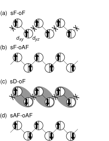
Figure 2: Spin and orbital ordering patterns in (a) the spin-ferro and orbital-ferro (sF-oF), (b) the spin-ferro and orbital-antiferro (sF-oAF), (c) the spin-dimer and orbital-ferro (sD-oF), and (d) the spin-antiferro and orbital-antiferro (sAF-oAF) states. Circles denote the lattice sites, and two separated spaces inside them denote two different orbital states $d_{xy}$ and $d_{yz}$ as indicated in (a). Arrows denote spins, and gray ovals in (c) represent the spin-singlet pairs. Crosses in (a) and (c) denote the disconnected bonds by the ferro-type orbital ordering. See the text for details.

The ground-state energy for each ordered state is calculated by replacing the spin and orbital-isospin operators in Eq. (5) by the following expectation values;

$$\langle\mbox{\boldmath$S$}_{i}\cdot\mbox{\boldmath$S$}_{i+1}\rangle=\frac{1}{4} \mbox{for sF pairs},$$ (15)

$$\langle\mbox{\boldmath$S$}_{i}\cdot\mbox{\boldmath$S$}_{i+1}\rangle=-\frac{3}{4} \mbox{for sD pairs},$$ (16)

$$\langle\mbox{\boldmath$S$}_{i}\cdot\mbox{\boldmath$S$}_{i+1}\rangle=-s \mbox{for sAF pairs},$$ (17)

where $s$ is a positive parameter less than $3/4$ (we do not need the precise value of $s$), and

$$\langle T_{i}T_{i+1}\rangle=\frac{1}{4},\ \langle T_{i}\rangle=\pm\frac{1}{2} \mbox{for oF pairs},$$ (18)

$$\langle T_{i}T_{i+1}\rangle=-\frac{1}{4},\ \langle T_{i}\rangle=\pm\frac{(-1)^{i}}{2} \mbox{for oAF pairs},$$ (19)

respectively. The obtained ground-state energies per site for the states (a)-(d) are

$$E_{\rm sF-oF}=0,$$ (20)

$$E_{\rm sF-oAF}=-J\left(A+\frac{B}{4}\right),$$ (21)

$$E_{\rm sD-oF}=-J\frac{C}{2},$$ (22)

$$E_{\rm sAF-oAF}=-J(A-sB),$$ (23)

respectively.

We compare Eqs. (20)-(23) by using Eqs. (8)-(11) and obtain

$$(E_{\rm sF-oAF}\ \mbox{or}\ E_{\rm sD-oF})<E_{\rm sAF-oAF}<E_{\rm sF-oF}.$$ (24)

Hence, the ground state is either (b) sF-oAF or (c) sD-oF state. From the equation of $E_{\rm sF-oAF}=E_{\rm sD-oF}$, we obtain the critical value of $\eta$ for the transition between the two phases as

$$\eta_{\rm c}=\frac{1}{3}(\sqrt{73}-8)\simeq 0.18.$$ (25)

Namely, we have the ground-state phase transition between the sD-oF and sF-oAF phases by changing $\eta$; the sD-oF (sF-oAF) phase is stable for $\eta<\eta_{\rm c}$ ($\eta>\eta_{\rm c}$). Hence, for a realistic value of $\eta\sim 0.1$, the ground state is predicted to be the sD-oF phase within the mean-field argument. This will be confirmed by the numerical calculations in Sec. IV. We will also show that the sF-oAF state is realized for $\eta>\eta_{\rm c}$ in Appendix B.

The $\eta$-controlled phase transition is understood by the competition between the spin superexchange interaction and the Hund’s-rule coupling. The former comes from the perturbation process within the same orbitals and favors the spin-singlet state. Anderson1959 The latter enhances the energy gain from the perturbation process between different orbitals and stabilizes the sF-oAF state. It is known that the sF-oAF state is favored by a finite Hund’s-rule coupling ($\eta>0$) in multiorbital systems with transfer integrals $t^{11}=t^{22}\neq 0$ between all the NN sites. Roth1966 ; Inagaki1973 In the present systems, the specific form of the transfer integrals due to the zig-zag lattice structure gives a chance to stabilize the sD-oF state in the small $\eta$ regime.

III.2 High-temperature para phase

At high temperatures, both spin and orbital are disordered. We here examine spin and orbital correlations in the para phase by a mean-field type argument.

First, to focus on the spin degree of freedom, we replace the orbital isospin operators in the effective model (5) with their mean values, i.e., $T_{i}\to\langle T_{i}\rangle=0$ and $T_{i}T_{i+1}\to\langle T_{i}T_{i+1}\rangle$. The resultant effective spin Hamiltonian reads

$$\mathcal{H}_{\rm s}^{\rm MF}=\sum_{i}\left(J_{i,i+1}^{\rm s}\mbox{\boldmath$S$}_{i}\cdot\mbox{\boldmath$S$}_{i+1}-K_{i,i+1}^{\rm s}\right),$$ (26)

where

$$J_{i,i+1}^{\rm s} = J\left[\frac{1}{4}(C-2B)+(C+2B)\langle T_{i}T_{i+1}\rangle\right],$$ (27)

$$K_{i,i+1}^{\rm s} = \frac{J}{4}\left[\frac{1}{4}(C+8A)+(C-8A)\langle T_{i}T_{i+1}\rangle\right].$$ (28)

In the high-temperature limit, $\langle T_{i}T_{i+1}\rangle$ becomes zero and the effective spin exchange constant becomes

$$J_{i,i+1}^{\rm s}(T\to\infty)=\frac{J}{4}(C-2B),$$ (29)

which is positive for $\eta\sim 0.1$ and independent of $i$. Hence, we end up with a 1D AF spin Heisenberg model.

On the other hand, we can also consider a reduced Hamiltonian for the orbital degree of freedom by replacing the spin operators in the model (5) with their mean values. The result is

$$\mathcal{H}_{\rm o}^{\rm MF}=\sum_{i}\left[J_{i,i+1}^{\rm o}T_{i}T_{i+1}-L_{i,i+1}^{\rm o}(T_{i}+T_{i+1})-K_{i,i+1}^{\rm o}\right],$$ (30)

where

$$J_{i,i+1}^{\rm o} = J\left[\left(2A-\frac{C}{4}\right)+(C+2B)\langle\mbox{\boldmath$S$}_{i}\cdot\mbox{\boldmath$S$}_{i+1}\rangle\right],$$

(31)

$$L_{i,i+1}^{\rm o} = (-1)^{i}J\frac{C}{2}\left(\frac{1}{4}-\langle\mbox{\boldmath$S$}_{i}\cdot\mbox{\boldmath$S$}_{i+1}\rangle\right),$$ (32)

$$K_{i,i+1}^{\rm o} = \frac{J}{4}\left[\left(2A+\frac{C}{4}\right)-(C-2B)\langle\mbox{\boldmath$S$}_{i}\cdot\mbox{\boldmath$S$}_{i+1}\rangle\right].$$

In the high-temperature limit, $\langle\mbox{\boldmath$S$}_{i}\cdot\mbox{\boldmath$S$}_{i+1}\rangle=0$ and the effective isospin coupling constant becomes

$$J_{i,i+1}^{\rm o}(T\to\infty)=J\left(2A-\frac{C}{4}\right).$$ (34)

This coupling constant is also positive for $\eta\sim 0.1$, and therefore, we obtain a 1D antiferro-type Ising isospin model. [Note that the second term in Eq. (30) cancels out when $\langle\mbox{\boldmath$S$}_{i}\cdot\mbox{\boldmath$S$}_{i+1}\rangle=0$.]

The above arguments indicate that both spin and orbital correlations are antiferro type in the high-temperature limit in our effective model (1). On the contrary, as discussed in Sec. III.1, the ground state is either the sF-oAF or sD-oF state. This suggests that either spin or orbital correlation has to change from antiferro to ferro type as decreasing temperature. It is implied by Eq. (27) that development of antiferro-type orbital correlations $\langle T_{i}T_{i+1}\rangle<0$ may change the sign of $J_{i,i+1}^{\rm s}$ from positive (antiferro) to negative (ferro). In a similar way, Eq. (31) suggests that development of AF spin correlations $\langle\mbox{\boldmath$S$}_{i}\cdot\mbox{\boldmath$S$}_{i+1}\rangle<0$ may induce the sign change of $J_{i,i+1}^{\rm o}$. In this manner, the spin and orbital correlations compete with each other. The mean-field-level argument is clearly insufficient to clarify the competition, and we will employ the more powerful numerical analysis in the next section.

IV Numerical Analysis

IV.1 Method

To study thermodynamic properties of the model (1), we apply the quantum transfer matrix (QTM) methodBetsuyaku1984 combined with the mean-field treatment of the JT distortions. Here, we describe the scheme of our analysis.

Since the present model (1) is highly 1D anisotropic, it is justified to treat the weak interchain coupling $\mathcal{H}_{\perp}$ as the mean fieldImry1975 in the form

$$\tilde{\mathcal{H}}_{\perp}=\lambda\sum_{\langle i,j\rangle}Q_{i}\tilde{Q}_{j}=-z|\lambda|\sum_{i}Q_{i}^{2},$$ (35)

where $\tilde{Q}_{j}$ is the mean-field value of the JT distortion at site $j$ and $z$ is the number of NN chains, i.e., $z=4$ in the present materials. As a result, the total Hamiltonian, $\mathcal{H}_{\rm so}+\mathcal{H}_{\rm JT}+\tilde{\mathcal{H}}_{\perp}$, is reduced to an effective 1D spin-orbital-lattice coupled model in the form

$$\tilde{\mathcal{H}} = \mathcal{H}_{\rm so}+\gamma\sum_{i}Q_{i}T_{i}+\frac{1-2z|\lambda|}{2}\sum_{i}Q_{i}^{2}$$ (36)

$$= \mathcal{H}_{\rm so}+\bar{\gamma}\sum_{i}\bar{Q}_{i}T_{i}+\frac{1}{2}\sum_{i}\bar{Q}_{i}^{2},$$

where the JT coupling and distortion are rescaled as $\bar{\gamma}=\gamma/\sqrt{1-2z|\lambda|}$ and $\bar{Q}_{i}=\sqrt{1-2z|\lambda|}Q_{i}$, respectively. For later use, we define the JT stabilization energy as

$$\Delta_{\rm JT}=\bar{\gamma}^{2}/8,$$ (37)

which is the energy gain by the JT distortion in the absence of $\mathcal{H}_{\rm so}$.

The optimal values of the JT distortions $\{\bar{Q}_{i}\}$ are determined in a self-consistent way. We start from an initial guess of $\{\bar{Q}_{i}\}$ and calculate the expectation values of the isospin $\langle T_{i}\rangle$ by applying the QTM method to the effective 1D model $\tilde{\mathcal{H}}$. Note that the QTM calculation is numerically exact and includes all the fluctuations in spin and orbital degrees of freedom for a given set of $\{\bar{Q}_{i}\}$. See Appendix A for the details of the QTM method. The obtained values of $\langle T_{i}\rangle$ are used to determine $\{\bar{Q}_{i}\}$ self-consistently. The self-consistent equation is obtained by the energy minimization $\delta\langle\mathcal{H}\rangle/\delta\bar{Q}_{i}=0$ which gives

$$\bar{Q}_{i}^{\rm new}=-\bar{\gamma}\langle T_{i}\rangle.$$ (38)

The values of $\{\bar{Q}_{i}^{\rm new}\}$ are used as inputs for the next QTM calculation. We iterate the procedure until $\{\bar{Q}_{i}\}$ converge to optimal values.

Thermodynamic properties are obtained for the optimal values of $\{\bar{Q}_{i}\}$. We calculate the magnetization per site,

$$m=\frac{1}{L}\sum_{i}\langle S^{z}_{i}\rangle,$$ (39)

and the average values of NN spin and orbital correlations,

$$C_{\rm s} = \frac{1}{L}\sum_{i}\langle\mbox{\boldmath$S$}_{i}\cdot\mbox{\boldmath$S$}_{i+1}\rangle,$$ (40)

$$C_{\rm o} = \frac{1}{L}\sum_{i}\langle T_{i}T_{i+1}\rangle,$$ (41)

respectively, where $L$ is the length of the chain. We also define the NN spin correlations on odd and even bonds as

$$C_{\rm s}^{\rm odd} = \frac{2}{L}\sum_{i\in{\rm odd}}\langle\mbox{\boldmath$S$}_{i}\cdot\mbox{\boldmath$S$}_{i+1}\rangle,$$ (42)

$$C_{\rm s}^{\rm even} = \frac{2}{L}\sum_{i\in{\rm even}}\langle\mbox{\boldmath$S$}_{i}\cdot\mbox{\boldmath$S$}_{i+1}\rangle,$$ (43)

respectively, to detect the spin dimerization. See Eqs. (52)-(56) in Appendix A for the calculation of these quantities. Besides, to calculate the magnetic susceptibility $\chi$, we perform the calculation within the same framework for the system under the external magnetic field whose Hamiltonian reads

$$\tilde{\mathcal{H}}-g\mu_{B}H\sum_{i}S_{i}^{z},$$ (44)

where $g$ is the $g$-factor and $\mu_{B}$ is the Bohr magneton, and $H$ is the external magnetic field. The susceptibility is obtained from the numerical derivative of $m$ as

$$\chi=\frac{m(\Delta H)-m(0)}{\Delta H},$$ (45)

where we use $\Delta H=0.001J/(g\mu_{B})$.

The QTM method allows us to treat the system in the thermodynamic limit $L\to\infty$ directly (see Appendix A). Instead, the results contain a systematic error due to a finite Trotter number $M$. We need to check carefully the convergence of the results with increasing $M$. The values of $M$ used in the following calculations are up to $M=4$ for the case of $\bar{\gamma}=0$ while up to $M=3$ for $\bar{\gamma}>0$. Although these values of $M$ appear to be rather small, we will show that the $M$-convergence is excellent for the temperature range in the present study, $T\mathrel{\mathchoice{\lower 2.5pt\vbox{\halign{$\m@th\displaystyle\hfil#\hfil$\cr>\crcr\sim\crcr}}}{\lower 2.5pt\vbox{\halign{$\m@th\textstyle\hfil#\hfil$\cr>\crcr\sim\crcr}}}{\lower 2.5pt\vbox{\halign{$\m@th\scriptstyle\hfil#\hfil$\cr>\crcr\sim\crcr}}}{\lower 2.5pt\vbox{\halign{$\m@th\scriptscriptstyle\hfil#\hfil$\cr>\crcr\sim\crcr}}}}0.1J$.

IV.2 Results

In this section, we show our numerical results for thermodynamic properties of the model (1) obtained by the method in the previous section. In Sec. IV.2.1, we clarify nontrivial feedback effects between orbital and spin degrees of freedom in the absence of the JT coupling. In Sec. IV.2.2, we switch on the JT coupling, and compare our numerical results with the experimental data.

IV.2.1 Interplay between orbital and spin

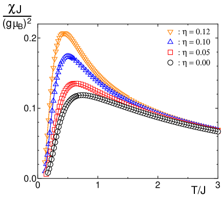
Figure 3: Temperature dependence of the magnetic susceptibility $\chi$ for $\eta=0.0,0.05,0.10$, and $0.12$. Symbols represent the results for $M=4$ while solid and dotted curves are those for $M=3$ and $M=2$, respectively.

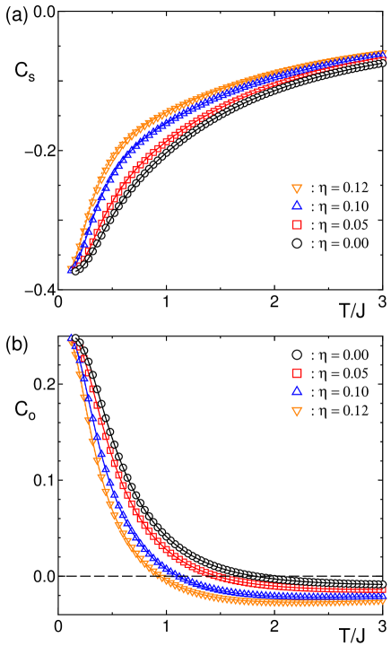
Figure 4: Temperature dependences of (a) the nearest-neighbor spin correlation $C_{\rm s}$ and (b) the nearest-neighbor orbital correlation $C_{\rm o}$ for $\eta=0.0,0.05,0.10$, and $0.12$. Symbols represent the results for $M=4$ while solid and dotted curves are those for $M=3$ and $M=2$, respectively.

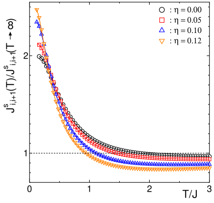
Figure 5: Effective spin exchange coupling $J_{i,i+1}^{\rm s}$ in Eq. (27) for $\eta=0.0,0.05,0.10$, and $0.12$. The results are scaled by their values in the high-temperature limit, $J_{i,i+1}^{\rm s}(T\to\infty)$.

First, we show our results in the absence of the JT coupling ($\bar{\gamma}=0$). In this case, the model is reduced to the 1D spin-orbital model $\mathcal{H}_{\rm so}$ [Eq. (5)], and we can obtain thermodynamic properties by performing the QTM calculation without any self-consistent iteration.

Figure 3 shows the results of the magnetic susceptibility $\chi$ in Eq. (45) for several values of $\eta$. Note that the results for different values of the Trotter number $M=2,3$, and $4$ almost coincide with each other as shown in the figure, which ensures the convergence of the QTM results in this parameter range. The magnetic susceptibility at high temperatures increases as temperature decreases, and exhibits a broad peak at some temperature. At lower temperatures, it decays rapidly and approaches zero as $T\to 0$. While the peak becomes sharper and shifts to a lower temperature region as $\eta$ increases, the rapid decay of $\chi$ at low temperatures is commonly observed. This indicates that our spin-orbital model $\mathcal{H}_{\rm so}$ in Eq. (5) exhibits the spin-singlet ground state in the small $\eta$ regime as predicted in Sec. III.1. (See Appendix B for the larger $\eta$ regime.)

To clarify the nature of the system in more detail, in Fig. 4, we show the results of NN spin and orbital correlations $C_{\rm s}$ and $C_{\rm o}$ defined in Eqs. (40) and (41), respectively. The $M$-dependence of the results is negligible also for these quantities. We note that at finite temperatures no true long-range order appears in the 1D spin-orbital model $\mathcal{H}_{\rm so}$, and hence the NN spin correlations are uniform, i.e., $C_{\rm s}=C_{\rm s}^{\rm odd}=C_{\rm s}^{\rm even}$. As $T\to 0$, the spin and orbital correlations converge to $C_{\rm s}=-3/8$ and $C_{\rm o}=1/4$, respectively. These are indeed the values expected in the sD-oF ground state shown in Fig. 2 (c), where $\langle\mbox{\boldmath$S$}_{i}\cdot\mbox{\boldmath$S$}_{i+1}\rangle$ takes the value of $-3/4$ or $0$ alternatively from bond to bond while $\langle T_{i}^{z}T_{i+1}^{z}\rangle=1/4$ for all bonds. Hence, we conclude that the ground state of the system is the sD-oF state in Fig. 2 (c) for the realistic values of $\eta\sim 0.1$, and the rapid decay of $\chi$ at low temperatures in Fig. 3 is due to the spin-singlet formation in the ground state.

Let us examine the finite-temperature behavior of $C_{\rm s}$ and $C_{\rm o}$ in Fig. 4. At high temperatures, both the spin and orbital correlations are negative, i.e., antiferro type, being consistent with the mean-field prediction in Sec. III.2. Here, the spin and orbital antiferro correlations compete with each other since the spin-antiferro correlation favors the orbital-ferro one and vice versa as indicated in the form of $\mathcal{H}_{\rm so}$ in Eq. (5). We find that in this range of $\eta$ the spin-antiferro correlation grows more rapidly than the orbital correlation as $T$ decreases. This growth of $C_{\rm s}$ suppresses $C_{\rm o}$ and causes the sign change of $C_{\rm o}$ from antiferro to ferro type. Once $C_{\rm o}$ becomes ferro type, $C_{\rm s}$ and $C_{\rm o}$ develop cooperatively, and eventually the ferro-type orbital correlation induces the spin-dimer formation in the ground state. These results clearly indicate that our model $\mathcal{H}_{\rm so}$ shows a nontrivial feedback effect between orbital and spin degrees of freedom at finite temperatures.

The strong interplay between orbital and spin also shows up in the temperature dependence of the magnetic susceptibility at high temperatures. There, we expect a deviation from the Curie-Weiss behavior due to the interplay since $J_{i,i+1}^{\rm s}$ depends on the NN orbital correlation $\langle T_{i}T_{i+1}\rangle$ as mentioned in Sec. III.2. The deviation can be monitored by the temperature dependence of the effective spin exchange coupling $J_{i,i+1}^{\rm s}$ in Eq. (27), since it gives an effective Curie-Weiss temperature $\Theta_{\rm CW}$. (In the mean-field approximation, $\Theta_{\rm CW}=J_{i,i+1}^{\rm s}/2$ in the 1D spin-$1/2$ system with NN interaction.)

In Fig. 5, we show the temperature dependence of $J_{i,i+1}^{\rm s}$ in Eq. (27) scaled by the value in the high-temperature limit. The results clearly show that $J_{i,i+1}^{\rm s}$ is temperature-dependent even in the temperature range where the Curie-Weiss fitting to the experimental data has been attempted in Ref. Isobe2002, . (The energy scale of $J$ will be estimated as $200-300$K from the fitting in the next section.) We need further careful considerations in the fitting of the experimental data of the magnetic susceptibility to estimate the model parameters.

IV.2.2 Comparison with experimental results

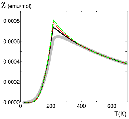
Figure 6: Comparison between numerical and experimental results of the magnetic susceptibility $\chi$. Solid, dotted, and dashed curves represent the numerical results for $(J,\eta,g,\Delta_{\rm JT})=(213$K$,0.05,1.85,86$K$)$, $(250$K$,0.10,1.87,90$K$)$, and $(296$K$,0.12,1.90,89$K$)$, respectively. Bold gray curve represents the experimental data in Ref. Isobe2002, .

Next, we show our results in the presence of the JT coupling, i.e., for the case of $\bar{\gamma}>0$ in Eq. (36), and compare them with experimental data quantitatively. The numerical results shown in the following are obtained from the self-consistent iteration of the QTM calculation with $M=3$, and we have confirmed the $M$-convergence of the results.

Figure 6 shows the results of the magnetic susceptibility $\chi$. The results show a singularity at some temperature and a sudden drop below there, which corresponds to the phase transition to the low-temperature sD-oF phase as discussed later. For comparison, we plot the experimental data for NaTiSi₂O₆,chi_m which increase as $T$ decreases at high temperatures and exhibit a sharp drop at $T_{\rm c}=210$K. The numerical results are obtained for several typical parameter sets estimated by the following fitting procedure: In our model, there are four parameters, i.e., the effective exchange coupling $J$, the ratio of Coulomb interactions $\eta=J_{\rm H}/U$, the $g$-factor $g$, and the JT coupling parameter $\bar{\gamma}$. For a certain value of $\eta$, we perform the two-parameter fitting by using $J$ and $g$ in the high-temperature regime of $400$K $<T<700$K, where the JT coupling $\bar{\gamma}$ is irrelevant in the present scheme of the calculation. Using the optimal values of $J$ and $g$, we determine $\bar{\gamma}$ to reproduce the critical temperature $T_{\rm c}=210$K. We thereby obtain the optimal set of $J$, $g$, and $\bar{\gamma}$ for a certain value of $\eta$.

In Fig. 6, we show the results of the fitting for $\eta=0.05,0.10$, and $0.12$ as typical examples. The estimates of the parameters are $(J,g,\Delta_{\rm JT})=(213$K$,1.85,86$K$)$, $(250$K$,1.87,90$K$)$, and $(296$K$,1.90,89$K$)$ for $\eta=0.05$, $0.10$, and $0.12$, respectively. As shown in the figure, the numerical results well reproduce the experimental data, except for a small deviation near $T_{\rm c}$ (discussed below). Although we cannot determine the best set of the parameter values only from the present fitting, we find that the estimates are quite reasonable in this $t_{2g}$ compound: The estimates of $J\sim 200-300$K are comparable to the estimate based on microscopic parameters in Sec. II. As for the $g$-factor, although there is no estimate for the present compound as far as we know, it is known that $g$ becomes slightly smaller than two in some $t_{2g}$ compounds, Kataev2003 ; Yamada1998 and therefore we believe that our estimates of $g$ are reasonable. Furthermore, the estimates of $\Delta_{\rm JT}\sim 90$K, which are smaller than the exchange energy $J$, also appear to be reasonable for $t_{\rm 2g}$ electron systems. (We will comment on the magnitude of $\Delta_{\rm JT}$ in the end of this section.) Therefore, we believe that our effective model (1) with realistic parameters can describe successfully the peculiar properties of the pyroxene compound NaTiSi₂O₆.

We note that the small deviation near $T_{\rm c}$ can be attributed to the approximation in the treatment of the JT distortion $\bar{Q}_{i}$: Our method to determine $\bar{Q}_{i}$ is not able to include effects of the short-range correlations and thermal fluctuations of lattice distortions, which tend to enhance the spin-singlet fluctuation and suppress the magnetic susceptibility $\chi$. It is therefore reasonable that our method overestimates $\chi$ around the critical point, where the effects become significant. We believe that better agreement near $T_{\rm c}$ may be obtained by including such effects, however this interesting problem is left for further study.

As shown in Fig. 6, the magnetic susceptibility of our model shows an exponential decay at low temperatures well below $T_{\rm c}$. We estimate the spin gap $\Delta_{\rm s}$ from the results below $0.5T_{\rm c}$ by the fitting function

$$\chi\propto\exp(-\Delta_{\rm s}/T).$$ (46)

The estimates of $\Delta_{\rm s}$ are $665,640$, and $638$K for $\eta=0.05,0.10$, and $0.12$, respectively. In experiment, the spin gap $\Delta_{\rm s}$ is estimated as $\sim 500$K,Isobe2002 which is comparable to our numerical results.

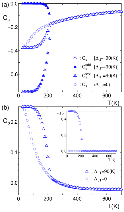
Figure 7: Temperature dependences of (a) the nearest-neighbor spin correlations $C_{\rm s}$, $C_{\rm s}^{\rm odd}$, and $C_{\rm s}^{\rm even}$, and (b) the nearest-neighbor orbital correlation $C_{\rm o}$ for $(J,\eta,\Delta_{\rm JT})=(250$K$,0.10,90$K$)$. Circles show the data for $\Delta_{\rm JT}=0$ for comparison. Inset in (b): Polarization of orbital isospin.

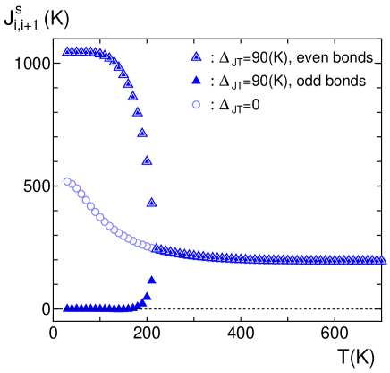
Figure 8: Temperature dependence of the effective spin exchange coupling $J_{i,i+1}^{\rm s}$ for $(J,\eta,\Delta_{\rm JT})=(250$K$,0.10,90$K$)$. Circles show the data for $\Delta_{\rm JT}=0$ for comparison.

Next, we show the results of the spin and orbital correlations in Fig. 7. Here, we plot only the results for the parameter set of $(J,\eta,\Delta_{\rm JT})=(250$K$,0.10,90$K$)$ as a typical example since essentially the same behavior is obtained for other parameter sets in Fig. 6.noneedg The correlations take the same values as those for $\Delta_{\rm JT}=0$ above $T_{\rm c}$. Below $T_{\rm c}$, the NN spin correlations on odd and even bonds, $C_{\rm s}^{\rm odd}$ and $C_{\rm s}^{\rm even}$, take different values and converge to $-3/4$ or $0$ as $T\to 0$. This indicates that the translational symmetry is broken in the spin-dimer phase. (Note that one of the doubly-degenerate ordered states is selected depending on the initial set of $\{\bar{Q}_{i}\}$ used in the self-consistent calculation.) On the other hand, the NN orbital correlation $C_{\rm o}$ is uniform, and goes to the value of $1/4$ as $T\to 0$. As shown in the inset of Fig. 7 (b), the isospin polarization $\langle T_{i}\rangle$ becomes finite below $T_{\rm c}$, indicating the long-range orbital ordering. These results explicitly show that the system below $T_{\rm c}$ is in the sD-oF phase in Fig. 2 (c).

In Fig. 8, we plot the effective spin exchange coupling $J_{i,i+1}^{\rm s}$, corresponding to Eq. (27) in the case of $\Delta_{\rm JT}=0$. For a finite $\Delta_{\rm JT}$, we have to keep the linear terms of $\langle T_{i}\rangle$ in the reduced spin Hamiltonian in Eq. (26), which give rise to an additional term $-J(-1)^{i}C/2\left(\langle T_{i}\rangle+\langle T_{i+1}\rangle\right)$ to $J_{i,i+1}^{\rm s}$ in Eq. (27). As shown in Fig. 8, the value of $J_{i,i+1}^{\rm s}$ deviates from that for $\Delta_{\rm JT}=0$ below $T_{\rm c}$, and takes two alternative values from bond to bond. This clearly shows the alternating behavior of the magnetic coupling in the spin-dimer state. At low temperatures $T\mathrel{\mathchoice{\lower 2.5pt\vbox{\halign{$\m@th\displaystyle\hfil#\hfil$\cr<\crcr\sim\crcr}}}{\lower 2.5pt\vbox{\halign{$\m@th\textstyle\hfil#\hfil$\cr<\crcr\sim\crcr}}}{\lower 2.5pt\vbox{\halign{$\m@th\scriptstyle\hfil#\hfil$\cr<\crcr\sim\crcr}}}{\lower 2.5pt\vbox{\halign{$\m@th\scriptscriptstyle\hfil#\hfil$\cr<\crcr\sim\crcr}}}}150$K, the dimerization is almost perfect, i.e., $J_{i,i+1}^{\rm s}$ on the weak bonds are almost zero. Hence, there the system consists of almost independent spin-singlet pairs. Note that $J_{i,i+1}^{\rm s}$ on the strong bonds is surprisingly enhanced up to $\sim 1000$K. The almost perfect dimerization and the enhanced exchange coupling are the unique aspects of the present spin-orbital-lattice coupled system.

Our estimates of the JT stabilization energy $\Delta_{\rm JT}\sim 90$K are considerably smaller than $T_{\rm c}=210$K as well as $J=200-300$K. This suggests that the critical temperature $T_{\rm c}$ is not determined mainly by the JT coupling, and that the balance of the JT coupling and the spin-orbital intersite interaction is important in this $t_{2g}$ electron system. Moreover, we note that the phase transition occurs below the temperature where the orbital correlation $C_{\rm o}$ changes its sign from negative (antiferro type) to positive (ferro type) as shown in Fig. 7 (b). This indicates an importance of the interplay and the feedback effect between spin and orbital in the present system. Therefore, we conclude that the pyroxene compounds are typical $t_{2g}$ electron systems where the JT energy scale is relatively small and the bare interplay between spin and orbital degrees of freedom plays a central role in the thermodynamic properties.

V summary and concluding remarks

In this paper, we have studied the effective spin-orbital-lattice coupled model which we derived to understand the peculiar phase transition to the spin-singlet state in $A$TiSi₂O₆ ($A$ = Na, Li). Using the mean-field-type analysis and the numerical quantum transfer matrix method, we have clarified that the interplay between spin and orbital degrees of freedom plays a central role in thermodynamic properties of the system. At high temperatures, both spin and orbital correlations are antiferro type and compete with each other. As temperature decreases, the antiferromagnetic spin correlation grows rapidly and yields the sign change of the orbital correlation from antiferro to ferro type so that the frustration is released. This ferro-type orbital correlation with the Jahn-Teller coupling finally causes a transition to the spin-dimer and orbital-ferro ordered phase. The feedback effect between orbital and spin degrees of freedom results in peculiar temperature dependence of the magnetic susceptibility. We have shown that the magnetic susceptibility data for NaTiSi₂O₆ can be explained by our effective model with realistic values of parameters.

The transition to the spin-singlet state in the present system shows several different aspects from conventional spin-Peierls systems. One is the temperature dependence of the magnetic susceptibility. In the present system, the rapid decay of the susceptibility due to the spin-singlet formation occurs even without a broad peak as a fingerprint of well-developed spin correlations. This is because the driving force of the transition is not the magnetoelastic interaction but the orbital-ferro correlations assisted by the Jahn-Teller distortion. However, this does not mean that the orbital-lattice physics is dominant as in $e_{g}$ electron systems such as CMR manganites. In the present $t_{2g}$ electron system, the Jahn-Teller energy scale is considerably smaller than the orbital and spin exchange interactions, and the orbital-ferro correlation is induced by the keen competition between the orbital and spin degrees of freedom. These illuminate a unique feature of the present $t_{2g}$ system, namely, there the interplay between orbital and spin appears explicitly without being dominated by Jahn-Teller physics.

Another peculiar aspect of the spin-dimer state in our model is that the spin-singlet pairs are formed on the longer Ti-Ti bonds rather than the shorter ones. In the present system, say, the $d_{xy}$ orbital ordering is concomitant with the flattening of TiO₆ octahedra in the $z$ direction which elongates Ti-Ti bonds in the $xy$ plane. Since the spin exchange interaction is strong between the nearest-neighbor sites in the $xy$ plane in this $d_{xy}$ ordered state, the spin-singlet dimers are formed on the longer Ti-Ti bonds. This aspect is clearly different from the conventional spin-Peierls systems in which the spin-singlet pairs are on shorter bonds. In our model, however, we take account of only the tetragonal Jahn-Teller mode which couples to $d_{xy}$ and $d_{yz}$ orbitals. For detailed comparisons with the experimental data which show much complicated lattice structure at low temperatures, it is necessary to include more general lattice distortions in our theory. In particular, we note that the magnetoelastic coupling can be substantial in the low-temperature orbital-ordered phase since the orbital-ferro ordering largely enhances the effective spin exchange coupling on strong bonds up to $\sim 1000$K as shown in Sec. IV.2.2. The magnetoelastic coupling will cause an opposite effect on the Ti-Ti bond lengths since it tends to shorten the spin-singlet Ti-Ti bonds. Further study is necessary to conclude the low-temperature lattice structure. Note that the inclusion of such magnetoelastic effect does not alter our conclusions on the mechanism of the phase transition because it becomes important only when the orbital-ferro ordering is well established far below the critical temperature.

In the present study, we have compared our results of the magnetic susceptibility with the experimental data for the Na compound NaTiSi₂O₆. There is another compound in this pyroxene family, i.e., LiTiSi₂O₆. The Li compound also shows the phase transition at $T_{\rm c}=230$K showing a sudden decay of the magnetic susceptibility below $T_{\rm c}$. Isobe2002 However, the susceptibility data show some extra anomalies probably due to impurity phases. We believe that our model describes essential physics in both the Na and Li compounds. Further experimental study including the sample refinement is desired to compare the data of Li compounds to our results.

As shown in Sec. III.1 and in Appendix B, the low-temperature phase of our effective model turns into the spin-ferro and orbital-antiferro ordered state for larger values of $\eta$ than the critical value of $\eta_{\rm c}\simeq 0.18$. The parameter $\eta$ is the ratio of the Hund’s-rule coupling to the intraorbital Coulomb repulsion, and is considered to be $\eta\sim 0.1<\eta_{\rm c}$ in the present compounds. Unfortunately, it is difficult to control the parameter $\eta$ experimentally, however, it may vary for different compounds to some extent. If $\eta$ becomes close to $\eta_{\rm c}$ in some compound, there would occur interesting phenomena related to the criticality of the phase transition at $\eta_{\rm c}$. One interesting example is the phase transition from the spin-dimer and orbital-ferro state to the spin-ferro and orbital-antiferro state by applying the external magnetic field. We have investigated this issue in our effective model, and indeed observed the field-induced phase transition. The results will be reported elsewhere. The experimental study of this issue is left for future study.

Appendix A Quantum Transfer Matrix method

In this appendix, we briefly review the algorithm of the QTM method.Betsuyaku1984 The QTM calculation is applied to the effective 1D model (36) in the self-consistent scheme as described in Sec. IV.1.

After the Suzuki-Trotter decomposition, the partition function is represented in terms of the transfer matrix as

$$Z={\rm Tr}~{}e^{-\beta\tilde{\mathcal{H}}}=\lim_{M\to\infty}{\rm Tr}~{}\prod_{n=1}^{L/2}\mathcal{T}_{M}$$ (47)

where $\beta=1/T$ (we set the Boltzmann constant $k_{\rm B}=1$), $M$ is the Trotter number, and $L$ is the system size. The transfer matrix $\mathcal{T}_{M}$ is given by

$$\mathcal{T}_{M}=\left[e^{-\beta\tilde{h}_{2n-1,2n}/M}e^{-\beta\tilde{h}_{2n,2n+1}/M}\right]^{M},$$ (48)

where $\tilde{\mathcal{H}}$ is decomposed into the summation of the local Hamiltonian $\tilde{h}_{i,i+1}$ for bond $(i,i+1)$. We omitted the index $n$ on the transfer matrix $\mathcal{T}_{M}$ since $\mathcal{T}_{M}$ for the present system is invariant under the two-site translation.

The advantage of the QTM method is that we can calculate thermodynamic quantities directly from the largest eigenvalue $\lambda_{\rm max}$ and the corresponding right $|v^{r}\rangle$ and left $\langle v^{l}|$ eigenvectors of $\mathcal{T}_{M}$.Suzuki1987 (Note that the eigenvectors $|v^{r}\rangle$ and $\langle v^{l}|$ are different in general since $\mathcal{T}_{M}$ is an asymmetric matrix.) The partition function of the infinite system is found to be $Z=\lim_{L\to\infty}\lambda_{\rm max}^{L/2}$, and consequently, the free energy per site can be obtained as

$$f=-\frac{1}{2\beta}\ln\lambda_{\rm max}.$$ (49)

Hence, once the value of $\lambda_{\rm max}$ is obtained, we can calculate any bulk quantity in the thermodynamic limit by taking the appropriate derivative of the free energy $f$.

Furthermore, we can calculate expectation values of site and bond operators.Wang1997 For instance, an expectation value of a product of operators $\mathcal{O}_{2n-1,2n}\mathcal{O}_{2n,2n+1}$ defined at sites $(2n-1,2n,2n+1)$ is obtained from the formula

$$\langle\mathcal{O}_{2n-1,2n}\mathcal{O}_{2n,2n+1}\rangle=\lim_{M\to\infty}\frac{\langle v^{l}|\mathcal{T}^{\mathcal{O}}_{M}|v^{r}\rangle}{\lambda_{\rm max}},$$ (50)

where

$$\mathcal{T}^{\mathcal{O}}_{M}=\mathcal{O}_{2n-1,2n}\mathcal{O}_{2n,2n+1}\mathcal{T}_{M}.$$ (51)

In the present study, we diagonalize the transfer matrix $\mathcal{T}_{M}$ numerically using the simple power method, which is known to be stable in the diagonalization of asymmetric matrix.Carlon1999 Then, using Eqs. (50) and (51), we calculate the magnetization $m$ [Eq. (39)] and the NN spin and orbital correlations $C_{\rm s}$ and $C_{\rm o}$ [Eqs. (40) and (41)] by

$$m = \frac{\langle S^{z}_{2n-1}\rangle+\langle S^{z}_{2n}\rangle}{2},$$ (52)

$$C_{\rm s} = \frac{\langle\mbox{\boldmath$S$}_{2n-1}\cdot\mbox{\boldmath$S$}_{2n}\rangle+\langle\mbox{\boldmath$S$}_{2n}\cdot\mbox{\boldmath$S$}_{2n+1}\rangle}{2},$$ (53)

$$C_{\rm o} = \frac{\langle T_{2n-1}T_{2n}\rangle+\langle T_{2n}T_{2n+1}\rangle}{2},$$ (54)

respectively. The NN spin correlations on odd and even bonds [Eqs. (42) and (43)] are given by

$$C_{\rm s}^{\rm odd} = \langle\mbox{\boldmath$S$}_{2n-1}\cdot\mbox{\boldmath$S$}_{2n}\rangle,$$ (55)

$$C_{\rm s}^{\rm even} = \langle\mbox{\boldmath$S$}_{2n}\cdot\mbox{\boldmath$S$}_{2n+1}\rangle,$$ (56)

respectively. In the spin-dimer phase, $C_{\rm s}^{\rm odd}$ and $C_{\rm s}^{\rm even}$ may take different values.

Appendix B transition to spin-F and orbital-AF phase

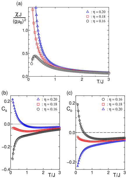
Figure 9: Temperature dependences of (a) the magnetic susceptibility $\chi$, (b) the nearest-neighbor spin correlation $C_{\rm s}$, and (c) the nearest-neighbor orbital correlation $C_{\rm o}$ for $\eta=0.16,0.18$ and $0.20$. Symbols represent the results for $M=4$ while solid and dotted curves are those for $M=3$ and $M=2$, respectively.

In this appendix, we discuss thermodynamic properties of the model (1) for larger values of $\eta$ than those studied in Sec. IV.2. There, the sF-oAF ground state is expected to be stable from the mean-field-type analysis in Sec. III.1.

We first discuss our numerical results for the spin-orbital model $\mathcal{H}_{\rm so}$, i.e., the effective model (36) without the JT coupling $\bar{\gamma}=0$, corresponding to the results in Sec. IV.2.1. Figure 9 (a) shows the results of the magnetic susceptibility $\chi$. The result for $\eta=0.16$ exhibits a sharp drop as $T\to 0$ similarly to the results in Fig. 3, indicating the spin-singlet ground state. On the contrary, for $\eta=0.18$ and $0.20$, $\chi$ exhibits a divergent behavior as $T\to 0$, suggesting that the ground state is magnetic. These suggest that there is a ground-state phase transition between nonmagnetic and magnetic phases at $\eta=\eta_{\rm c}\sim 0.18$.

To clarify the nature of the transition in more detail, we show the results of NN spin and orbital correlations $C_{\rm s}$ and $C_{\rm o}$ in Figs. 9 (b) and (c), respectively. The results for $\eta=0.16$ show similar features to those for smaller $\eta$ shown in Sec. IV.2, and indicate that the system exhibits the sD-oF ground state. For $\eta=0.20$, on the other hand, the antiferro-type orbital correlation $C_{\rm o}$ develops rapidly, yielding the sign change of the spin correlation $C_{\rm s}$. After the sign change, the two correlations grow cooperatively, and approach the values of $C_{\rm s}=1/4$ and $C_{\rm o}=-1/4$ as $T\to 0$. These are the values expected in the sF-oAF ground state shown in Fig. 2 (b). Hence, the system with $\eta=0.20$ exhibits the sF-oAF ground state. For $\eta=0.18$, $C_{\rm s}$ and $C_{\rm o}$ are both antiferro type and compete with each other down to the lowest temperature studied here. This suggests that $\eta=0.18$ is close to the phase boundary between the sD-oF and sF-oAF phases. Therefore, we conclude that the ground state of the spin-orbital model $\mathcal{H}_{\rm so}$ undergoes a phase transition between the sD-oF and sF-oAF phases at $\eta=\eta_{\rm c}\sim 0.18$. The critical value is in good agreement with the mean-field prediction in Sec. III.1.

In the case of a finite JT coupling, we have found that there occurs a finite-temperature phase transition to the low-temperature sF-oAF phase for $\eta>\eta_{\rm c}$ or to the sD-oF phase for $\eta<\eta_{\rm c}$. The details will be reported elsewhere.

References

- (1) Y. Tokura and N. Nagaosa, Science 288, 462 (2000).
- (2) M. Imada, A. Fujimori, and Y. Tokura, Rev. Mod. Phys. 70, 1039 (1998).
- (3) K. I. Kugel and D. I. Khomskii, Sov. Phys. Usp. 25, 231 (1982).
- (4) E. O. Wollan and W. C. Koehler, Phys. Rev. 100, 545 (1955); J. B. Goodenough, Phys. Rev. 100, 564 (1955).
- (5) S. Miyasaka, Y. Okimoto, M. Iwama, and Y. Tokura, Phys. Rev. B 68, 100406(R) (2003).
- (6) Y. Motome, H. Seo, Z. Fang, and N. Nagaosa, Phys. Rev. Lett. 90, 146602 (2003).
- (7) G. Khaliullin, P. Horsch, and A. M. Oleś, Phys. Rev. Lett. 86, 3879 (2001).
- (8) M. Isobe, E. Ninomiya, A. Vasil’ev, and Y. Ueda, J. Phys. Soc. Jpn. 71, 1423 (2002).
- (9) E. Ninomiya, M. Isobe, Y. Ueda, M. Nishi, K. Ohoyama, H. Sawa, and T. Ohama, Physica B 329-333, 884 (2003).
- (10) J. W. Bray, L. V. Interrante, I. S. Jacobs, J. C. Bonner, Extended Linear Chain Compounds vol.3, ed. by J. C. Miller (New York, Plenum Press, 1983) p.353; J. P. Boucher and L. P. Regnault, J. Phys. I (France) 6, 1939 (1996); K. Uchinokura, J. Phys: Condens. Matter 14, 195 (2002).
- (11) N. Katoh, J. Phys. Soc. Jpn. 68, 258 (1999).
- (12) M. J. Konstantinović, J. van den Brink, Z. V. Popović, V. V. Moshchalkov, M. Isobe, and Y. Ueda, Phys. Rev. B 69, 020409(R) (2004).
- (13) K. I. Kugel and D. I. Khomskii, Sov. Phys. Solid. State 17, 285 (1975).
- (14) P. Millet, F. Mila, F. C. Zhang, M. Mambrini, A. B. Van Oosten, V. A. Pashchenko, A. Sulpice, and A. Stepanov, Phys. Rev. Lett. 83, 4176 (1999).
- (15) We note that the transfer integrals may be modified by the JT distortion. We neglect the small corrections in the present study.
- (16) H. Tsunetsugu and Y. Motome, Phys. Rev. B 68, 060405(R) (2003); Y. Motome and H. Tsunetsugu, preprint (cond-mat/0406039), to be published in Phys. Rev. B.
- (17) T. Mizokawa and A. Fujimori, Phys. Rev. B 54, 5368 (1996).
- (18) Y. Imry, P. Pincus, and D. Scalapino, Phys. Rev. B 12, 1978 (1975); H. J. Schulz, Phys. Rev. Lett. 77, 2790 (1996).
- (19) P. W. Anderson, Phys. Rev. 115, 2 (1959).
- (20) L. M. Roth, Phys. Rev. 149, 306 (1966).
- (21) S. Inagaki and R. Kubo, Int. J. Magnetism 4, 139 (1973); S. Inagaki, J. Phy. Soc. Jpn. 39, 596 (1975).
- (22) H. Betsuyaku, Phys. Rev. Lett. 53, 629 (1984); Prog. Theor. Phys. 73, 319 (1985).
- (23) The experimental data shown in Fig. 6 correspond to in Ref. Isobe2002, which contain only the intrinsic contributions after the subtractions of a Curie contribution from magnetic impurities and a constant term due to core-electron diamagnetism and the Van Vleck paramagnetism.
- (24) V. Kataev, J. Baier, A. Möller, L. Jongen, G. Meyer, and A. Freimuth, Phys. Rev. B 68, 140405(R) (2003).
- (25) I. Yamada, H. Manaka, H. Sawa, M. Nishi, M. Isobe, and Y. Ueda, J. Phys. Soc. Jpn. 67, 4269 (1998).
- (26) Note that the results of the correlations are independent of the value of .
- (27) M. Suzuki and M. Inoue, Prog. Theor. Phys. 78, 787 (1987); M. Inoue and M. Suzuki, Prog. Theor. Phys. 79, 645 (1988).
- (28) X. Wang and T. Xiang, Phys. Rev. B 56, 5061 (1997).
- (29) E. Carlon, M. Henkel, and U. Schollwöck, Eur. Phys. J. B 12, 99 (1999).